An Efficiency Method for Assessment of Shear Stress in Prismatic Beams with Arbitrary Cross-Sections

Abstract

The dimensions of a bearing structure tend to be designed as slender as possible to ensure aesthetics and to save material, which makes the structure more susceptible to damage caused by shear forces. When the structure is subjected to an earthquake, the shear failure is even the primary mode of failure. Research on shear stress has always been of great interest to scientists. This paper presents an efficient method for the assessment of the shear stress for prismatic beams with arbitrary cross-section. The numerical method implemented in a MATLAB environment is validated by analyzing five examples. The study shows the efficiency and reliability of the numerical method, which allows for more precise analysis and design of cross-sections. Therefore, significant savings of material can be reached, which will have a positive impact on our environment and which can help sustainable growth.

1. Introduction

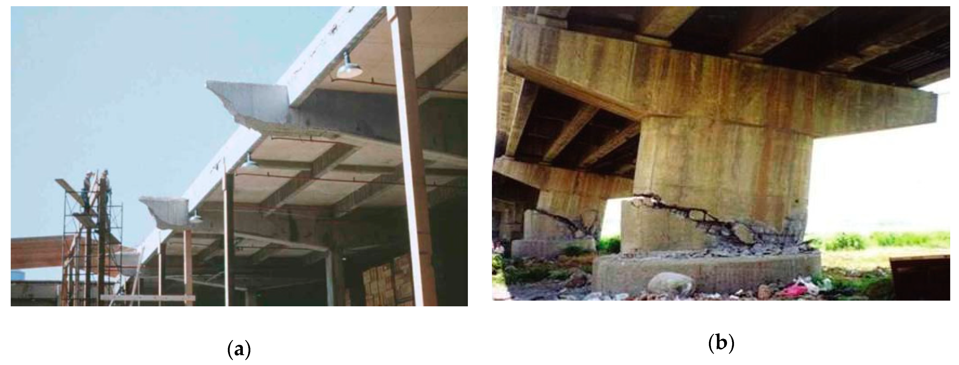
Engineers tend to design the dimensions of load-bearing structural elements as slender as possible to ensure aesthetic appearance and to reduce material consumption requirements. Considering the fact that nowadays most load-bearing systems of buildings and bridges are created by reinforced prestressed concrete structures, the decrease of the need for concrete would certainly reduce carbon dioxide (CO2) emissions and global warming and, therefore, would contribute to keep economic development sustainable. On the other hand, the effort to design slender and aesthetic structures makes them more susceptible to damage by shear stress. Figure 1a shows the shear failure cases of the American Air force warehouses in 1955 and 1956 [1]. Figure 1b depicts the shear failure of a squat bridge pier during a Taiwan 1999 earthquake [2].

The accurate determination of shear stress is one of the factors to ensure the sustainability of a structure, which is a problem that attracts researchers. Many scientists [3,4,5,6,7,8,9,10,11,12,13,14,15,16,17,18,19,20,21,22,23] have studied numerical methods dealing with shear stress due to bending and torsion.

Gruttmann, F. et al. [3,4] used the finite element method to evaluate shear stress by using the warping function, which is more convenient than using the Prandtl’s stress function [24,25] when considering multiply connected domain. Gruttmann, F. [4] introduced a method for computing the shear correction factors for Timoshenko beams with arbitrary cross-sections. Gruttmann’s numerical method has been implemented into an enhanced version of the program FEAP [5,6,26] which used 4-noded isoparametric elements. Fialko, S. Yu et al. [7] developed a numerical method using constant triangular elements to solve the Saint Venant problem of torsion, and torsionless bending of prismatic bars is realized in the SCAD software [8].

Garcia, J.M.B. et al. [9,10] developed a method of analysis to deal with arbitrary cross-section and general non-linear material (i.e., concrete). Poliotti, M. [11] improved Garcia’s method’s computation speed using b-spline interpolation to reduce unknowns when solving problems. Yoon, K. et al. [14] proposed a new efficient warping displacement model. The model can be used for discontinuously varying cross-section beams. However, the method does not take into account the multiply connected domains. A comparison of methods for the strength assessment of prestressed reinforced concrete cross-sections with respect to the interaction of tensile and shear forces and bending and torsional moments was performed by Navrátil, J. et al. [13]. Genoese, A. [14] proposed a method for determining only the shear stress for nonuniform torsion. Jog, C.S. [15] demonstrated a method for determining the shear stress due to bending and torsion for inhomogeneous materials. However, the coupling of bending and torsion was not considered. Urbański, A. [16] studied a finite element method considering the interaction of internal force components with arbitrary cross-section. However, the multiply connected domain was not considered. Beheshti, A. [17] contributed to a method of determining the shear stress due to torsion, including strain-gradient elasticity.

Sapountzakis, E.J. et al. [18,19] proposed the nonuniform torsion solution and the general transverse shear loading problem of beams of the arbitrary cross-section with the boundary element method. Barone, G. [20] used the complex variable boundary element method to evaluate shear stress caused by torsion and flexure in beams. Paradiso, M. [21] introduced a numerical method based on the boundary element method to determine shear stress in the Saint Venant theory of beam. A boundary approach labeled line element-less method was recently shown to solve the Saint Venant’s flexure–torsion problem for isotropic material and arbitrary cross-sections by Di Paola, M. et al. [22].

In summary, the existing literature has constructed a large number of numerical methods for the shear stress problem. All of the works demonstrate the feasibility and effectiveness only in academia. Currently, only Gruttmann’s method [3,4] has been developed into the FEAP program [6] of the University of California, Berkeley, and Allplan Bridge [23]. Fialko’s method [7] is similar to that of Grutmmann, which has been developed as a module in the SCAD commercial software [8]. It means the methods of Gruttmann and Fialko are practical. However, the authors found that using a 4-noded isoparametric element in FEAP and constant strain triangle element in SCAD takes a lot of time for meshing to achieve optimal results. So, the authors decided to develop a new numerical method (NMB) based on the work of Gruttmann using the nine-noded isoparametric element. The validation examples were performed to show the reliability and efficiency of the sustainability design of NMB.

2. Solution Procedure by Numerical Method

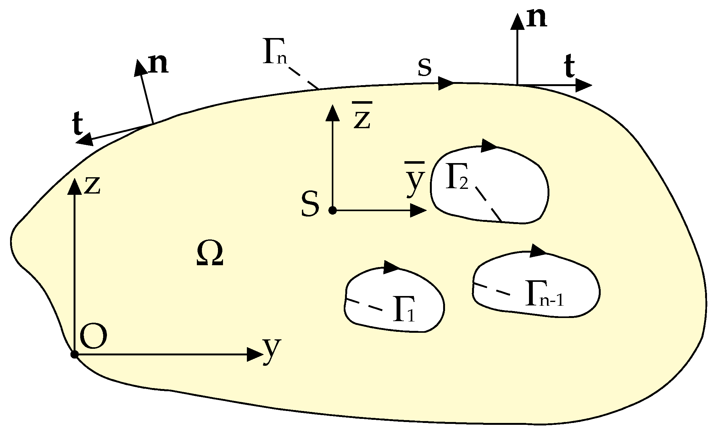
Consider a prismatic bar with an arbitrary constant cross-section. The longitudinal axis is the x-axis, and the cross-sections lie in the y–z plane, see Figure 2. The parallel system $\overline{y}=y-y_S$ and $\overline{z}=z-z_S$ intersects at the centroid. The multiply connected domain $\mathsf{\Omega }$ is bounded by ${\mathsf{\Gamma }}_1$, ${\mathsf{\Gamma }}_2$,… ${\mathsf{\Gamma }}_{n-1}$, ${\mathsf{\Gamma }}_n$. On ${\mathsf{\Gamma }}_1$, ${\mathsf{\Gamma }}_2$,… ${\mathsf{\Gamma }}_{n-1}$, ${\mathsf{\Gamma }}_n$ the right-handed orthogonal basis system is defined with tangent vector $t$ and outward normal vector $n={[n_y,n_z]}^T$. With $t$, the orientation of the associated coordinate s is uniquely defined.

2.1. Saint Venant Torsion Problem

The displacement field $u={[u_x,u_y,u_z]}^T$ is given by

$$u_x=\alpha {\omega }^T{,}^{}{u}_y=-{\beta }_{x}z{,}^{}{u}_z=-{\beta }_{x}y,$$

(1)

where ${\beta }_x$ is torsion angle and $\alpha =\frac{d{\beta }_x}{dx}$, ${\omega }^T(y,z)$ denotes warping function for torsion. Here, the following constraint is required:

$${\displaystyle \underset{\mathsf{\Omega }}{\int }{\omega }^{T}dA}=0$$

(2)

.

The shear stresses are defined by

$${\tau }_{xy}=G\alpha \left(\frac{\partial {\omega }^T}{\partial y}-z\right){,}^{}{\tau }_{xz}=G\alpha \left(\frac{\partial {\omega }^T}{\partial z}+y\right).$$

(3)

The polar second moment of area can read as

$$I_T={\displaystyle \underset{\mathsf{\Omega }}{\int }\left[\left(\frac{\partial {\omega }^T}{\partial z}+y\right)y-\left(\frac{\partial {\omega }^T}{\partial y}-z\right)z\right]dA}.$$

(4)

The strong form of the boundary value problem is described by

$$\begin{array}{l}\frac{{\partial }^2{\omega }^T}{{\partial }^{2}y}+\frac{{\partial }^2{\omega }^T}{{\partial }^{2}z}=0\hspace{1em}in\mathsf{\Omega },\\ n_y\frac{\partial {\omega }^T}{\partial y}+n_z\frac{\partial {\omega }^T}{\partial z}=n_{y}z-n_{z}y\hspace{1em}on\partial \mathsf{\Omega },\end{array}$$

(5)

where

$$n_y=\frac{dz}{ds},n_z=-\frac{dy}{ds}.$$

(6)

Using the Galerkin method, with test function $\eta \in V$ with $V=\{\eta \in H^1(\mathsf{\Omega }),\eta =0on\partial {\mathsf{\Omega }}_{{\omega }^T}\}$, Gruttmann, F. [3] transformed the strong form (5) to the weak form as below:

$$G({\omega }^T,\eta )={\displaystyle \underset{\mathsf{\Omega }}{\int }\left(\frac{\partial {\omega }^T}{\partial y}\frac{\partial \eta }{\partial y}+\frac{\partial {\omega }^T}{\partial z}\frac{\partial \eta }{\partial z}\right)dA-{\displaystyle \underset{\partial \mathsf{\Omega }}{\oint }(n_{y}z-n_{z}y)\eta ds}}=0$$

(7)

.

2.2. Saint Venant Torsionless Bending Problem

From reference [4], the relation between shear forces $Q_y$ and $Q_z$ and the corresponding, bending-related normal stress component, ${\sigma }_x$, is given in the format

$$\frac{\partial {\sigma }_x}{\partial x}=f_0(y,z)=a_1\overline{y}+a_2\overline{z},$$

(8)

where proportionality factors $a_1$ and $a_2$ are defined as

$$\left[\begin{array}{c}{a}_1\\ a_2\end{array}\right]=\frac{1}{A_{\overline{y}\overline{y}}{A}_{\overline{z}\overline{z}}-A_{\overline{y}\overline{z}}^2}\left[\begin{array}{cc}{A}_{\overline{z}\overline{z}}& -A_{\overline{y}\overline{z}}\\ -A_{\overline{y}\overline{z}}& A_{\overline{y}\overline{y}}\end{array}\right]\left[\begin{array}{l}{Q}_y\\ Q_z\end{array}\right],$$

(9)

where $Q_y$ and $Q_z$ are related to shear stress component via

$$Q_y={\displaystyle \underset{(\mathsf{\Omega })}{\int }{\tau }_{xy}dA}{,}^{}{Q}_z={\displaystyle \underset{(\mathsf{\Omega })}{\int }{\tau }_{xz}dA},$$

(10)

where $A_{\overline{y}\overline{y}}{,}^{}{A}_{\overline{z}\overline{z}}{,}^{}{A}_{\overline{y}\overline{z}}$ are the second-order area moments, defined by

$$A_{\overline{y}\overline{y}}={\displaystyle \underset{(\mathsf{\Omega })}{\int }{\overline{y}}^2}dA{,}^{}{A}_{\overline{z}\overline{z}}={\displaystyle \underset{(\mathsf{\Omega })}{\int }{\overline{z}}^2}dA{,}^{}{A}_{\overline{y}z}={\displaystyle \underset{(\mathsf{\Omega })}{\int }\overline{y}\overline{z}}dA.$$

(11)

The shear stresses are defined by

$${\tau }_{xy}=\frac{\partial {\omega }^B}{\partial y}-f_1(z){,}^{}{\tau }_{xz}=\frac{\partial {\omega }^B}{\partial z}-f_2(y),$$

(12)

where ${\omega }^B$ is warping function due to torsionless bending. Furthermore, the functions

$$f_1(z)=-\frac{v}{2(1+\nu )}{a}_1{(z-z_o)}^2{,}^{}{f}_2(y)=-\frac{\nu }{2(1+\nu )}{a}_2{(y-y_0)}^2,$$

(13)

where $v$ is Poisson’s ratio. The parameters $y_o{,}^{}{z}_o$ are derived from the following formulations:

$$y_o=\frac{B_{yy}}{2B_y}{,}^{}{z}_o=\frac{B_{zz}}{2B_z},$$

(14)

where

$$\begin{array}{l}{B}_y={\displaystyle \underset{(\mathsf{\Omega })}{\int }\left(\frac{\partial {\omega }^T}{\partial z}+y\right)\mathrm{y}dA}{,}^{}{B}_{yy}={\displaystyle \underset{(\mathsf{\Omega })}{\int }\left(\frac{\partial {\omega }^T}{\partial z}+y\right){\mathrm{y}}^{2}dA},\\ B_z={\displaystyle \underset{(\mathsf{\Omega })}{\int }\left(\frac{\partial {\omega }^T}{\partial y}-z\right)\mathrm{z}dA}{,}^{}{B}_{zz}={\displaystyle \underset{(\mathsf{\Omega })}{\int }\left(\frac{\partial {\omega }^T}{\partial y}-z\right){\mathrm{z}}^{2}dA},\end{array}$$

(15)

where ${\omega }^T$ is warping function due to torsion.

The strong form of the boundary value problem is described by

$$\begin{array}{l}\frac{{\partial }^2{\omega }^B}{{\partial }^{2}y}+\frac{{\partial }^2{\omega }^B}{{\partial }^{2}z}+f_o(y,z)=0in\mathsf{\Omega },\\ {\tau }_{xy}{n}_y+{\tau }_{xz}{n}_z=0on\partial \mathsf{\Omega },\end{array}$$

(16)

where

$$n_y=\frac{dz}{ds}{,}^{}{n}_z=-\frac{dy}{ds}.$$

(17)

Using the Galerkin method, with test function $\eta \in V$ with $V=\{\eta \in H^1(\mathsf{\Omega }){,}^{}\eta =0on\partial {\mathsf{\Omega }}_{{\omega }^B}\}$, Gruttmann, F. [4] transformed the strong form (16) to the weak form as below:

$$G({\omega }^B,\eta )={\displaystyle \underset{\mathsf{\Omega }}{\int }\left(\frac{\partial {\omega }^B}{\partial y}\frac{\partial \eta }{\partial y}+\frac{\partial {\omega }^B}{\partial z}\frac{\partial \eta }{\partial z}\right)dA-{\displaystyle \underset{\mathsf{\Omega }}{\int }\left(f_0\eta +f_1\frac{\partial \eta }{\partial y}+f_2\frac{\partial \eta }{\partial z}\right)}}dA=0$$

(18)

.

2.3. Finite Element Discretization

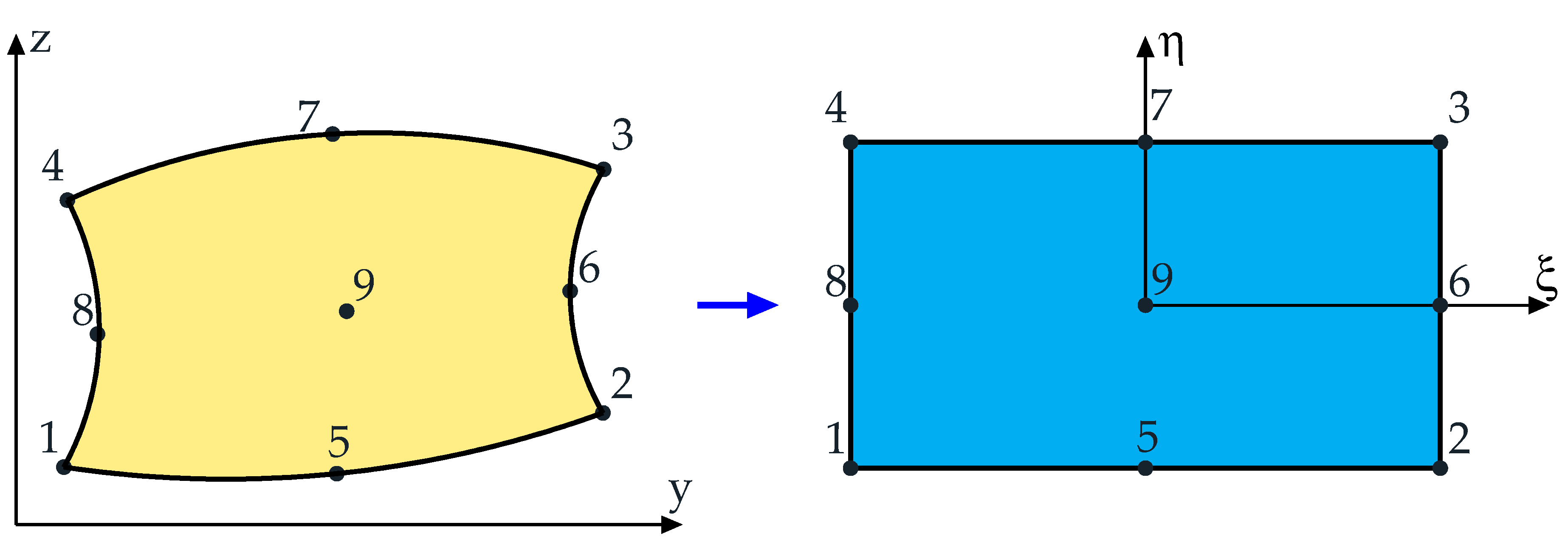
Consider the cross-section divided by nine-noded isoparametric quadrilateral elements. $x={[y,z]}^T$ and the unknown function ${\omega }^T$, ${\omega }^B$, and the test function $\eta$ are interpolated within a typical element using the same shape functions:

$$\begin{array}{l}{\mathbf{x}}^h={\displaystyle \sum _{I=1}^9{N}_I}\left(\xi ,\eta \right){\mathbf{x}}_I,{({\omega }^T)}^h={\displaystyle \sum _{I=1}^9{N}_I\left(\xi ,\eta \right){\omega }_I^T},\\ {({\omega }^B)}^h={\displaystyle \sum _{I=1}^9{N}_I\left(\xi ,\eta \right){\omega }_I^B},{(\eta )}^h={\displaystyle \sum _{I=1}^9{N}_I\left(\xi ,\eta \right){\eta }_I},\end{array}$$

(19)

where h denotes the approximate solution of the finite element method. $N_I(\xi ,\eta )$ denotes the shape function of the element. Figure 3 shows the nine-noded isoparametric quadrilateral element used in NMB. From reference [27], the shape functions $N_I(\xi ,\eta )$ of this element can be described as follows:

$$\begin{gathered} N_1(\xi ,\eta )=\frac{\xi (\xi -1)\eta (\eta -1)}{4},N_2(\xi ,\eta )=\frac{(\xi +1)\xi \eta (\eta -1)}{4},N_3(\xi ,\eta )=\frac{(\xi +1)\xi (\eta +1)\eta }{4}, \\ {N}_4(\xi ,\eta )=\frac{\xi (\xi -1)(\eta +1)\eta }{4},N_5(\xi ,\eta )=\frac{(\xi +1)(\xi -1)\eta (\eta -1)}{-2}, \\ {N}_6(\xi ,\eta )=\frac{(\xi +1)\xi (\eta +1)(\eta -1)}{-2},N_7(\xi ,\eta )=\frac{(\xi +1)(\xi -1)(\eta +1)\eta }{-2}, \\ {N}_8(\xi ,\eta )=\frac{\xi (\xi -1)(\eta +1)(\eta -1)}{-2},N_9(\xi ,\eta )=\frac{(\xi +1)(\xi -1)(\eta +1)(\eta -1)}{1}. \end{gathered}$$

(20)

Inserting the derivatives of ${({\omega }^T)}^h$, ${\eta }^h$ and ${({\omega }^B)}^h$, into the weak forms of (7) and (18), respectively, yields the finite element equations

$$\begin{array}{l}{\displaystyle \underset{e=1}{\overset{numel}{\cup }}{\displaystyle \sum _{I=1}^9{\displaystyle \sum _{K=1}^9\delta {\omega }_I^T(K_{IK}^e}}}{\omega }_K^T-F_I^{e(T)})=0,\\ {\displaystyle \underset{e=1}{\overset{numel}{\cup }}{\displaystyle \sum _{I=1}^9{\displaystyle \sum _{K=1}^9\delta {\omega }_I^B(K_{IK}^e}}}{\omega }_K^B-F_I^{e(B)})=0\end{array}$$

(21)

.

The operator ${\displaystyle \cup }$ describes the assembly and numel the total number of finite elements to solve the problem. The stiffness part, $K_{IK}^e$, to the nodes I and K as well as the right hand $F_I^{e(T)}$ and $F_I^{e(B)}$ yields

$$\begin{array}{ll}{K}_{IK}^e& ={\displaystyle \underset{{\mathsf{\Omega }}_e}{\int }\left(\frac{\partial N_I}{\partial y}\frac{\partial N_K}{\partial y}+\frac{\partial N_I}{\partial z}\frac{\partial N_K}{\partial z}\right)}d{A}_e\\ & ={\displaystyle \underset{-1}{\overset{1}{\int }}{\displaystyle \underset{-1}{\overset{1}{\int }}\left(\frac{\partial N_I}{\partial y}\frac{\partial N_K}{\partial y}+\frac{\partial N_I}{\partial z}\frac{\partial N_K}{\partial z}\right)\left|J\right|d\xi d\eta }}\\ & ={\displaystyle \sum _{p=1}^P{\displaystyle \sum _{q=1}^Q{w}_p{w}_q}}\left(\frac{\partial N_I}{\partial y}({\xi }_p,{\eta }_q)\frac{\partial N_K}{\partial y}({\xi }_p,{\eta }_q)+\frac{\partial N_I}{\partial z}({\xi }_p,{\eta }_q)\frac{\partial N_K}{\partial z}({\xi }_p,{\eta }_q)\right)\left|J({\xi }_p,{\eta }_q)\right|,\end{array}$$

(22)

$$\begin{array}{ll}{F}_I^{e(T)}& ={\displaystyle \underset{{\mathsf{\Omega }}_e}{\int }\left(\frac{\partial N_I}{\partial y}z-\frac{\partial N_I}{\partial z}y\right)}d{A}_e\\ & ={\displaystyle \underset{-1}{\overset{1}{\int }}{\displaystyle \underset{-1}{\overset{1}{\int }}\left(\frac{\partial N_I}{\partial y}z+\frac{\partial N_I}{\partial z}y\right)\left|J\right|d\xi d\eta }}\\ & ={\displaystyle \sum _{p=1}^P{\displaystyle \sum _{q=1}^Q{w}_p{w}_q}}\left(\frac{\partial N_I}{\partial y}({\xi }_p,{\eta }_q)z-\frac{\partial N_I}{\partial z}({\xi }_p,{\eta }_q)y\right)\left|J({\xi }_p,{\eta }_q)\right|,\end{array}$$

(23)

$$\begin{array}{ll}{F}_I^{e(B)}& ={\displaystyle \underset{{\mathsf{\Omega }}_e}{\int }\left(f_0{N}_I+f_1\frac{\partial N_I}{\partial y}+f_2\frac{\partial N_I}{\partial z}\right)}d{A}_e\\ & ={\displaystyle \underset{-1}{\overset{1}{\int }}{\displaystyle \underset{-1}{\overset{1}{\int }}\left(f_0{N}_I+f_1\frac{\partial N_I}{\partial y}+f_2\frac{\partial N_I}{\partial z}\right)\left|J\right|d\xi d\eta }}\\ & ={\displaystyle \sum _{p=1}^P{\displaystyle \sum _{q=1}^Q{w}_p{w}_q}}\left(f_0{N}_I({\xi }_p,{\eta }_q)+f_1\frac{\partial N_I({\xi }_p,{\eta }_q)}{\partial y}+f_2\frac{\partial N_I({\xi }_p,{\eta }_q)}{\partial z}\right)\left|J({\xi }_p,{\eta }_q)\right|,\end{array}$$

(24)

where $J$ denoted as Jacobian matrix is defined as

$$J=\left[\begin{array}{cc}\frac{\partial y}{\partial \xi }& \frac{\partial z}{\partial \eta }\\ \frac{\partial y}{\partial \xi }& \frac{\partial z}{\partial \eta }\end{array}\right],$$

(25)

where $w_p$ and $w_q$ are the weights and ${\xi }_p$ and ${\eta }_q$ are the integration points of the Gaussian integration technique.

We use 3 × 3 Gauss quadrature derived from the 1D case where the quadrature points are located at $-\sqrt{3/5}$, 0, and $\sqrt{3/5}$, and the corresponding weights are equal to 5/9, 8/9, and 5/9, respectively (see reference [26]).

The value ${\omega }_I^T$ and ${\omega }_I^B$ of one arbitrary nodal point I has to be value 0.

From reference [24], shear correction factor $\kappa$ is the ratio of the average strain on a section to the shear strain at the centroid. Gruttmann, F. [4] used it as the criterion to evaluate the convergence solutions to the Saint Venant torsionless bending problem. The shear correction factor ${\kappa }_y$, ${\kappa }_z$ is computed as

$${\kappa }_y=1/{\alpha }_y{,}^{}{\kappa }_z=1/{\alpha }_z,$$

(26)

where

$$\begin{array}{l}{\alpha }_y=\frac{A}{Q_y}\left[\frac{A_{{\omega }^B\overline{y}}{A}_{\overline{z}\overline{z}}-A_{{\omega }^B\overline{z}}{A}_{\overline{y}\overline{z}}}{A_{\overline{y}\overline{y}}{A}_{\overline{z}\overline{z}}-A_{\overline{y}\overline{z}}^2}+\frac{\nu }{2(1+\nu )}\frac{C_{zz}{A}_{\overline{z}\overline{z}}-C_{yy}{A}_{\overline{y}\overline{z}}}{A_{\overline{y}\overline{y}}{A}_{\overline{z}\overline{z}}-A_{\overline{y}\overline{z}}^2}\right],\\ {\alpha }_z=\frac{A}{Q_z}\left[\frac{A_{{\omega }^B\overline{z}}{A}_{\overline{y}\overline{y}}-A_{{\omega }^B\overline{y}}{A}_{\overline{y}\overline{z}}}{A_{\overline{y}\overline{y}}{A}_{\overline{z}\overline{z}}-A_{\overline{y}\overline{z}}^2}+\frac{\nu }{2(1+\nu )}\frac{C_{yz}{A}_{\overline{y}\overline{y}}-C_{zz}{A}_{\overline{y}\overline{z}}}{A_{\overline{y}\overline{y}}{A}_{\overline{z}\overline{z}}-A_{\overline{y}\overline{z}}^2}\right],\end{array}$$

(27)

where

$$C_{yy}={\displaystyle \underset{(\mathsf{\Omega })}{\int }{\tau }_{xz}{(y-y_0)}^2}dA{,}^{}{C}_{zz}={\displaystyle \underset{(\mathsf{\Omega })}{\int }{\tau }_{xy}{(z-z_0)}^2}dA,$$

(28)

$$A_{{\omega }^B\overline{z}}={\displaystyle \underset{(\mathsf{\Omega })}{\int }{\omega }^B\overline{z}dA}{,}^{}{A}_{{\omega }^B\overline{y}}={\displaystyle \underset{(\mathsf{\Omega })}{\int }{\omega }^B\overline{y}dA}.$$

(29)

3. Validation Examples

The objective of this section is to show the assessment of NMB and its performance. For this purpose, five special problems derived from references [3,4,7,24] were studied and their results compared with those predicted by NMB implemented in MATLAB R2015a. The finite element discretization was realized by employing the SAP2000 software version 14.2 [28] and MATLAB of an in-house code. We used a part of the open-source library presented in reference [29].

3.1. Rectangular Cross-Section

To test the problem of torsion, we considered a bar of square cross-section subjected to the torsion moment $M_T=1$ [MN.m] with the length of the edge 1 [m]. The comparison of the values of maximum shear stress and polar second moment of area obtained by analytical solution [24] was performed. The visualization of the distribution of shear stress was also displayed.

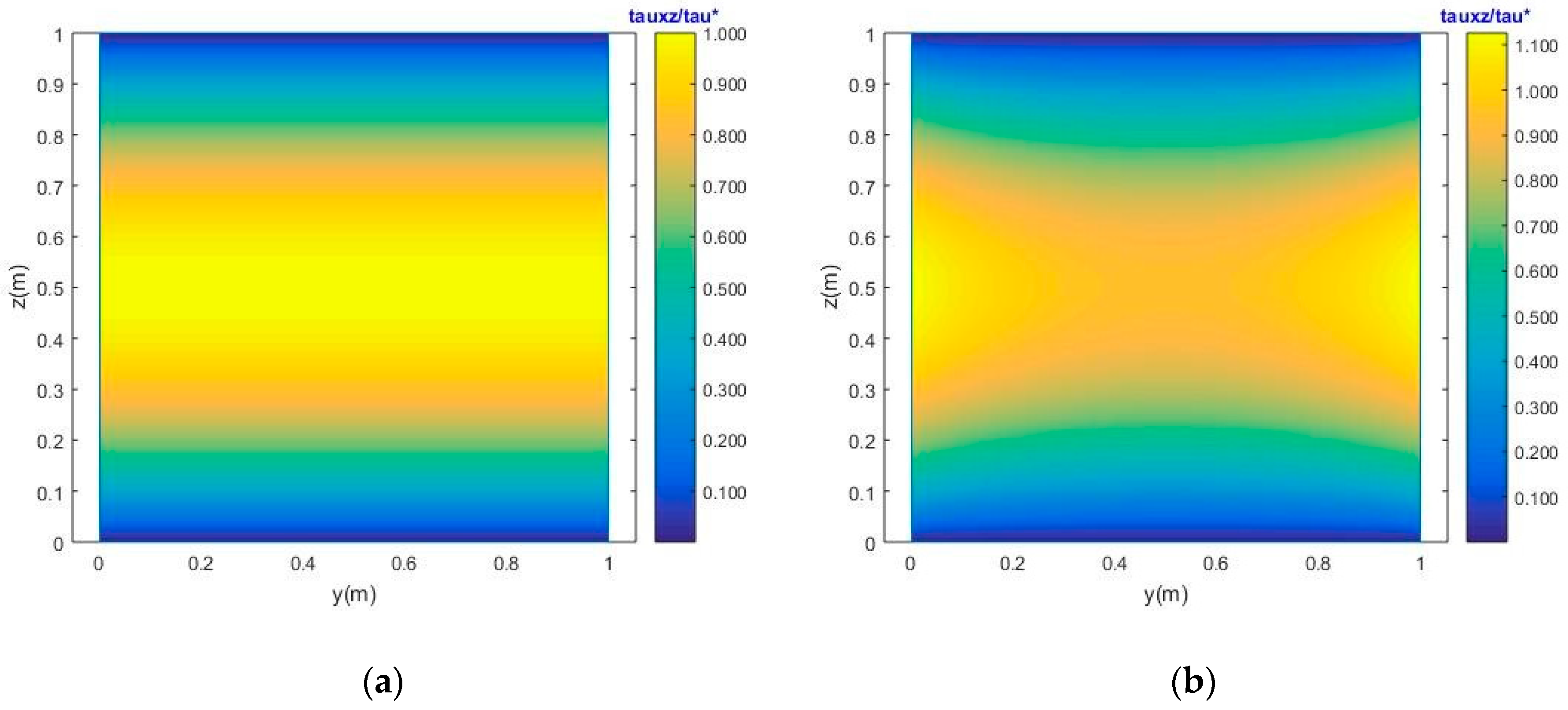
We checked the problem of the torsionless bending of a rectangular cross-section on the basis of the comparison with the results of [3,4]. Shear correction factors ${\kappa }_z=1/{\alpha }_z$ were the evaluated criteria. We investigated the rectangular cross-section due to $Q_z=1$ [kN] with the dimensions ($h=2$ [m], $b=1$ [m]), ($h=1$ [m], $b=1$ [m]), ($h=0.5$ [m], $b=1$ [m]), ($h=0.25$ [m], $b=1$ [m]) corresponding with the ratio ($h/b=2{,}^{}1{,}^{}0.5{,}^{}0.25$) and with different Poisson’s ratio $\nu =0{,}^{}0.25{,}^{}0.5$. The distribution of shear stress with two Poisson’s ratios, $\nu =0{,}^{}0.25$, was also shown.

The maximum shear stress corresponding to the maximum slope of the membrane is at the middle points of the long sides of the rectangle [24]. It means the distribution of shear stress of the square section decreases from the middle point of the edge to the center. Figure 4 shows a good agreement with the theoretical results.

It is clear from

Table 1. Square section in torsion.

Factors	Analytical [24]	NMB	Error, %
${\tau }_{\max }$ [MPa]	4.80769	4.81162	0.082
$I_T$ [m4]	0.1406	0.14058	0.0142

that the results of the maximum shear stress and the polar second moment of area obtained from NMB are in good agreement with the theoretical solution [24].

Figure 5 shows the distribution of the shear stress with Poisson’s ratios $\nu =0{;}^{}0.25$. The stress concentration at $z=0$, $y=\pm b/2$ can be seen clearly. We can see the distribution of stress over the width of the section is not constant when the Poisson’s ratio v ≠ 0.

It can be observed from

Table 2. Shear correction factors ${\kappa }_z$ with $h/b=2$.

Factors	FEAP [4]	NMB	Error, %
$\nu =0$	0.8333	0.833335	0.0
$\nu =0.25$	0.8331	0.833041	0.0
$\nu =0.5$	0.8325	0.832519	0.0

,

Table 3. Shear correction factors ${\kappa }_z$ with $h/b=1$.

Factors	FEAP [4]	NMB	Error, %
$\nu =0$	0.8333	0.833335	0.0%
$\nu =0.25$	0.8295	0.829486	0.0%
$\nu =0.5$	0.8228	0.822729	0.0%

,

Table 4. Shear correction factors ${\kappa }_z$ with $h/b=0.5$.

Factors	FEAP [4]	NMB	Error, %
$\nu =0$	0.8333	0.833335	0.0
$\nu =0.25$	0.7961	0.796066	0.0
$\nu =0.5$	0.7375	0.737438	0.0

and

Table 5. Shear correction factors ${\kappa }_z$ with $h/b=0.25$.

Factors	FEAP [4]	NMB	Error, %
$\nu =0$	0.8333	0.833335	0.0
$\nu =0.25$	0.6308	0.630724	0.0
$\nu =0.5$	0.4404	0.440378	0.0

that the results of shear correction factors ${\kappa }_z$ obtained from rectangular cross-section with different $h/b$ and Poisson’s ratio ν from NMB are in good agreement with FEAP results [4].

3.2. Cross-Section with Varying Width

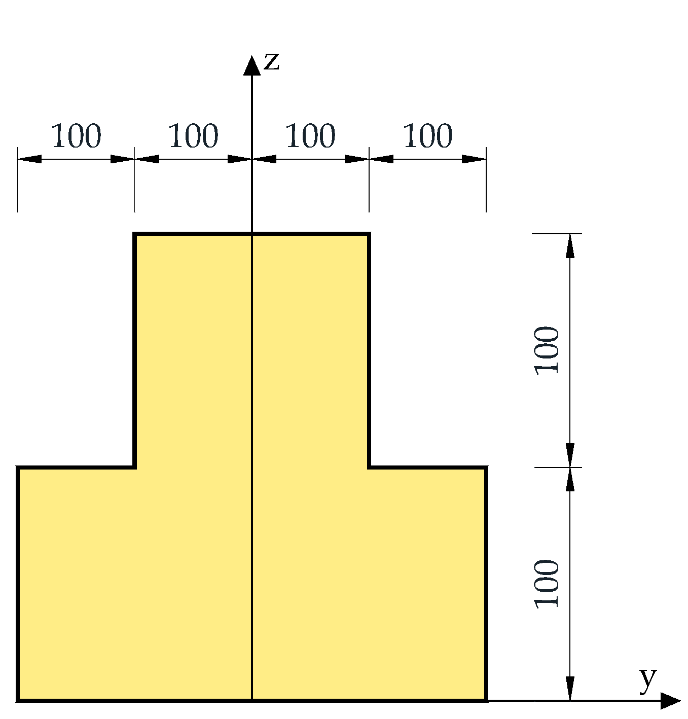
The next example is performed with a cross-section with varying width [3,4]. Figure 6 shows the dimension of the cross-section.

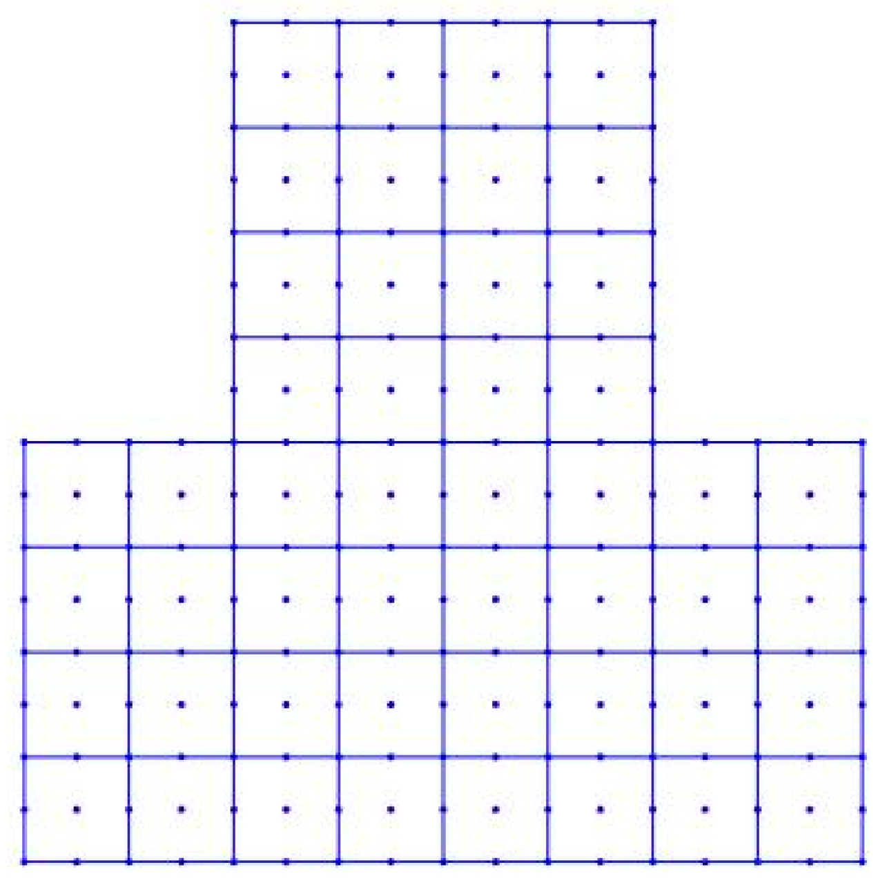
FEAP [3] used 480 elements to get the convergence values, while NMB used only 48 elements (225 nodes). Figure 7 shows the discretization of the cross-section with varying width by NMB.

Table 6. Shear correction factors ${\kappa }_y,{\kappa }_z$ with $\nu =0$.

Factors	FEAP [4]	NMB	Error, %
${\kappa }_y$	0.7395	0.7409	0.19
${\kappa }_z$	0.6767	0.6788	0.31

,

Table 7. Shear correction factors ${\kappa }_y,{\kappa }_z$ with $\nu =0.25$.

Factors	FEAP [4]	NMB	Error, %
${\kappa }_y$	0.7355	0.7372	0.23
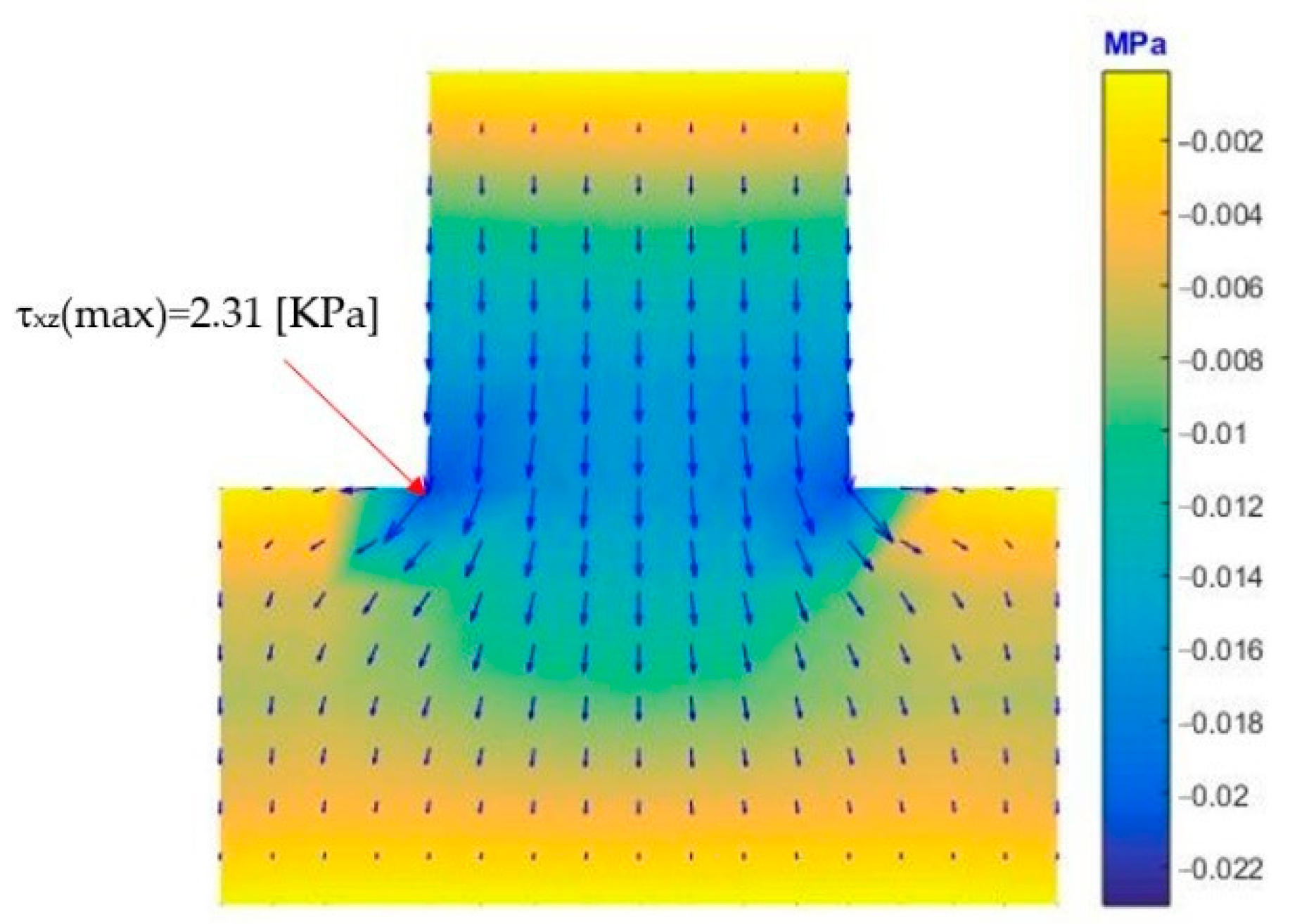
${\kappa }_z$	0.6753	0.6774	0.31

and

Table 8. Shear correction factors ${\kappa }_y,{\kappa }_z$ with $\nu =0.5$.

Factors	FEAP [4]	NMB	Error, %
${\kappa }_y$	0.7294	0.7307	0.18
${\kappa }_z$	0.6727	0.6749	0.33

show the errors of the shear correction factors between FEAP and NMB are under 0.33%. Figure 8 shows the distribution of the shear stress ${\tau }_{xz}$ and the resulting shear stresses with Poisson’s ratio $\nu =0.2$ due to $Q_z=-1$ [kN]. The maximum shear stress ${\tau }_{xz}$ of FEAP and NMB is 2.321 KPa and 2.31 KPa, respectively.

3.3. Crane Rail A100

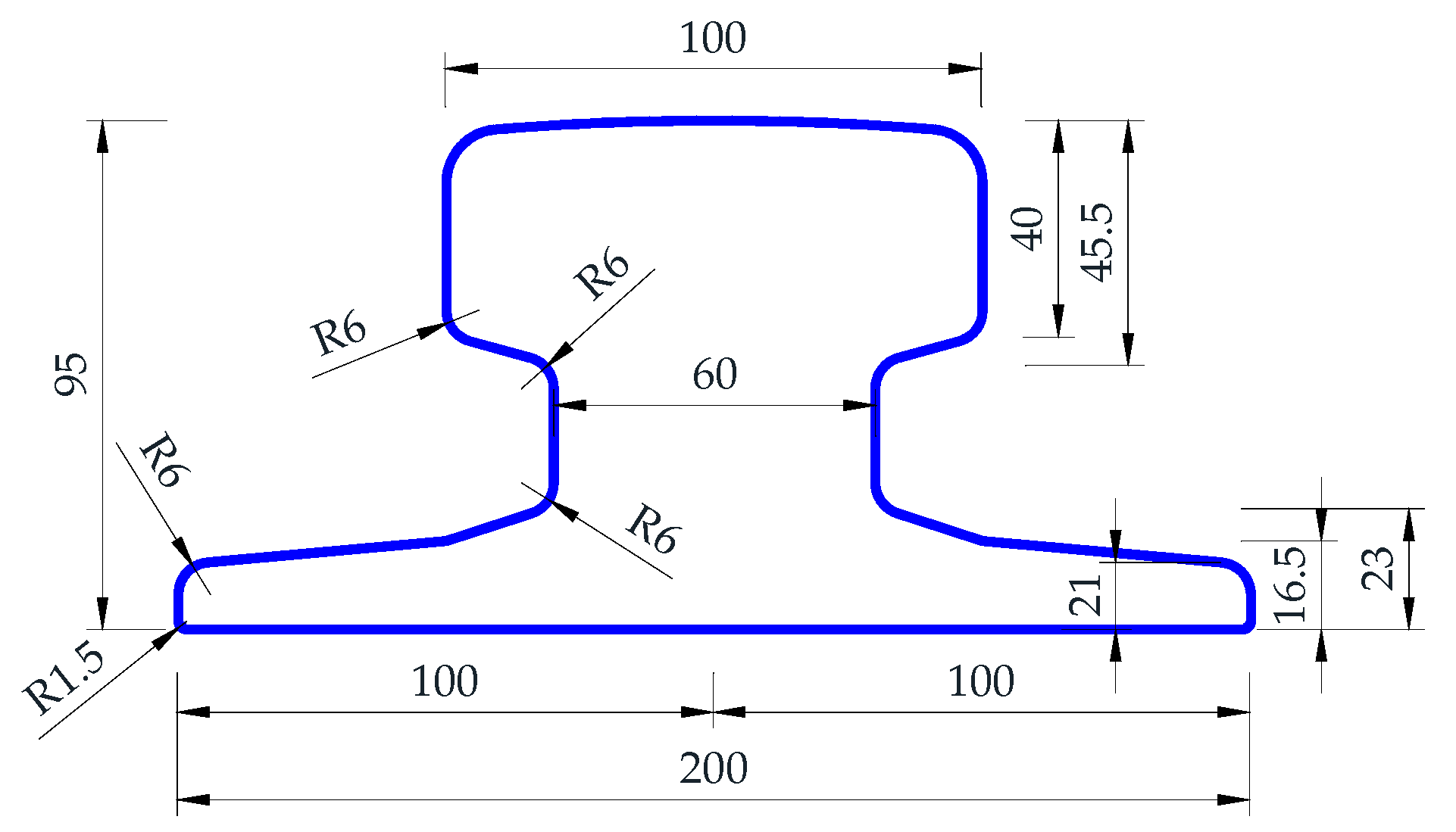
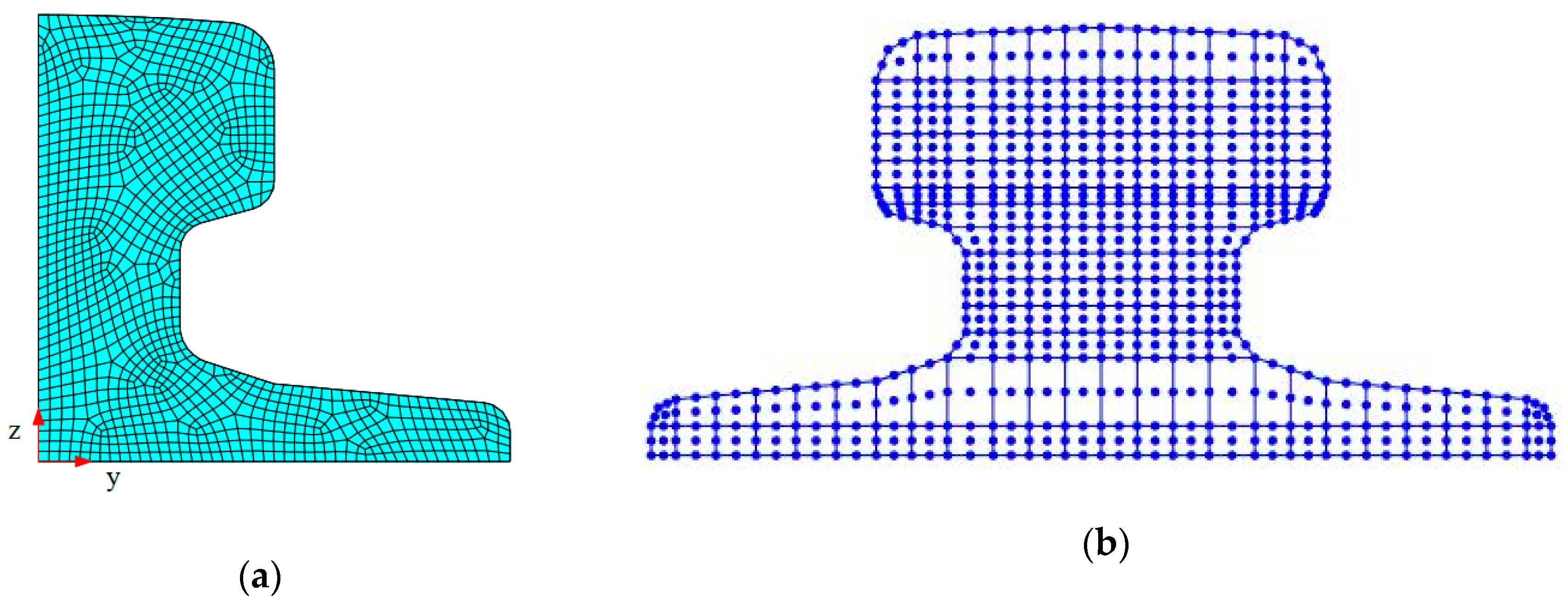
The next example concerns crane rail section A100 according to German standard DIN 536. Figure 9 depicts the dimension of the cross-section. FEAP [3] used 66,934 elements to get convergence values. NMB meshed the crane rail section by 172 elements (773 nodes) to obtain the convergence result. Figure 10a,b illustrate the crane rail section’s discretization by FEAP and NMB, respectively.

In

Table 9. The polar second moment of area and the parameter $z_0$

Factors	FEAP [3]	NMB	Error, %
$I_T$ [cm4]	670.7	675.9	0.77
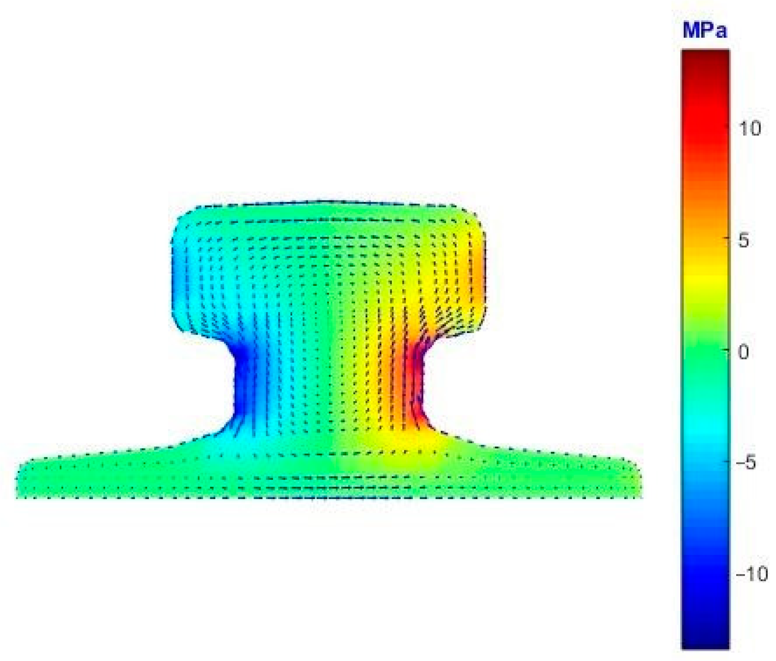
$z_0$ [cm]	5.078	5.060	0.35

, we present a comparison of the polar second moment of area, the parameter $z_0$ between NMB with FEAP. The error is under 0.77%. Figure 11 shows the distribution of the shear stress ${\tau }_{xz}$ and the resulting shear stresses due to $M_T=1$ [kN.m].

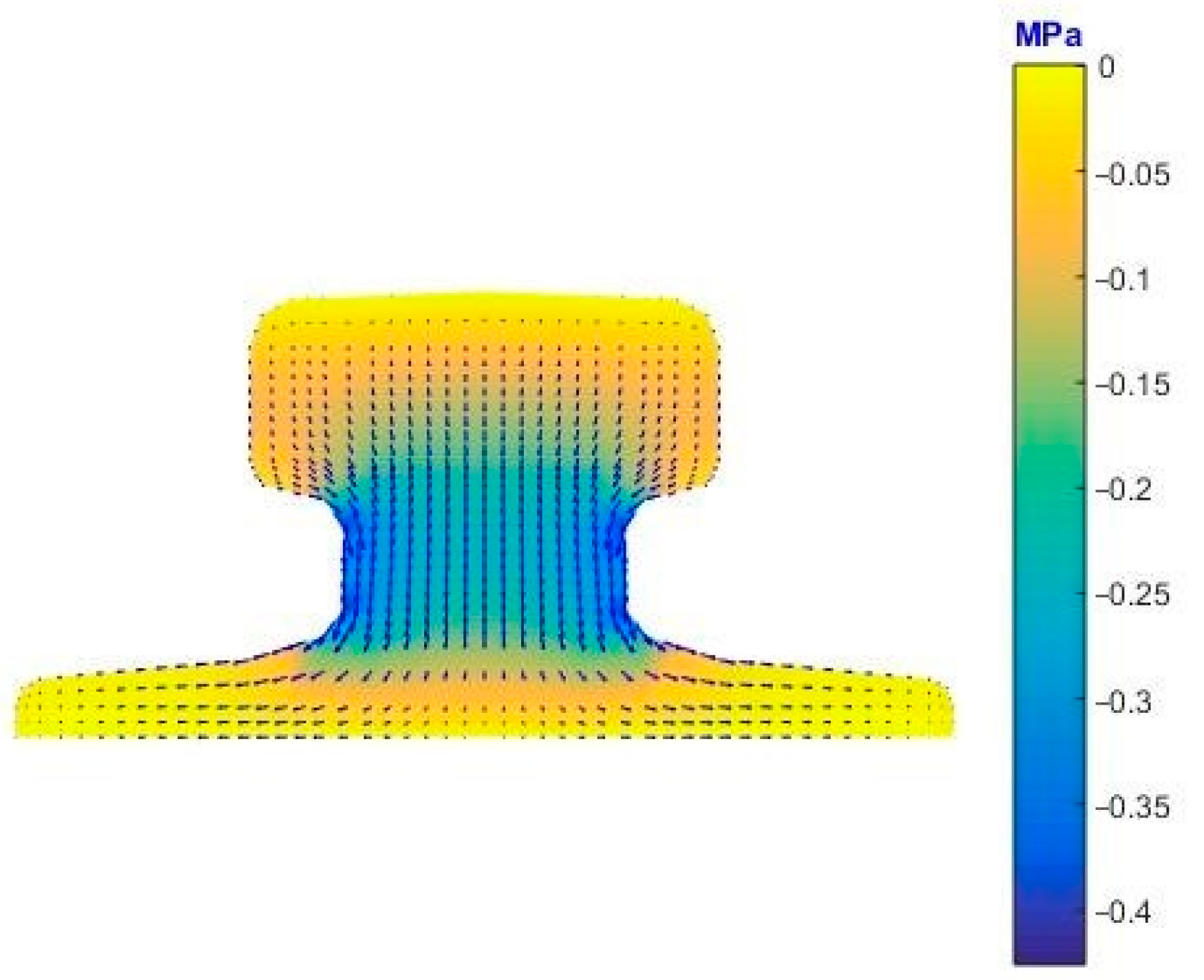
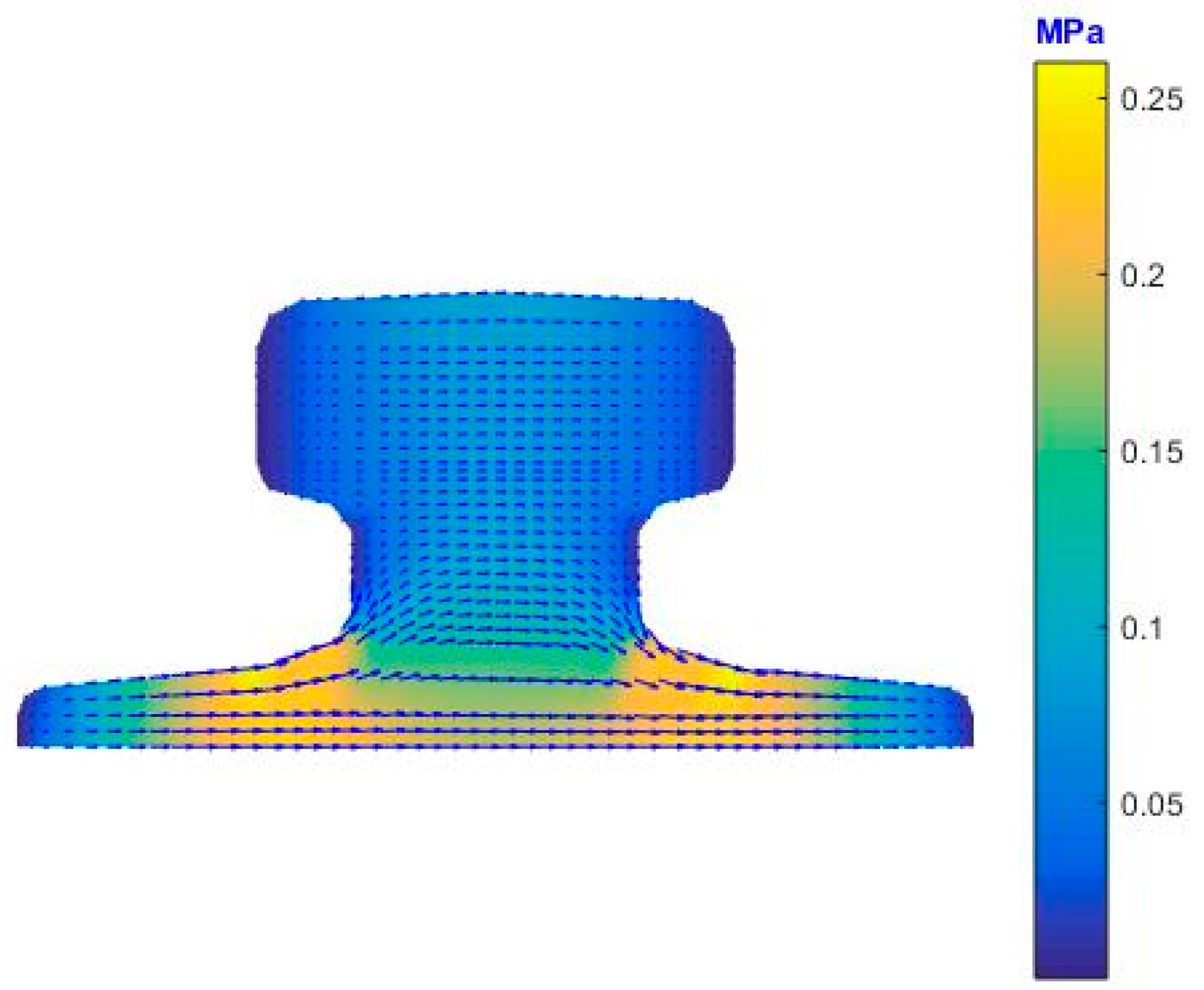
Figure 12 shows the distribution of the shear stress ${\tau }_{xz}$ and the resulting shear stresses with Poisson’s ratio $\nu =0.3$ due to $Q_z=-1$ [kN]. The maximum shear stress ${\tau }_{xz}$ of FEAP and NMB is 0.41 MPa and 0.42 MPa, respectively. Figure 13 depicts the distribution of the shear stress ${\tau }_{xy}$ and the resulting shear stresses with Poisson’s ratio $\nu =0.3$ due to $Q_y=1$ [kN].

Table 10. Shear correction factors ${\kappa }_y,{\kappa }_z$ with $\nu =0$.

Factors	FEAP [4]	NMB	Error, %
${\kappa }_y$	0.6845	0.6867	0.32
${\kappa }_z$	0.4474	0.4506	0.71

and

Table 11. Shear correction factors ${\kappa }_y,{\kappa }_z$ with $\nu =0.3$.

Factors	FEAP [4]	NMB	Error, %
${\kappa }_y$	0.6836	0.6859	0.34
${\kappa }_z$	0.4468	0.4499	0.69

show the errors of the shear correction factors between FEAP and NMB are under 0.71%.

3.4. Bridge Cross-Section with Doubly Connected Domain

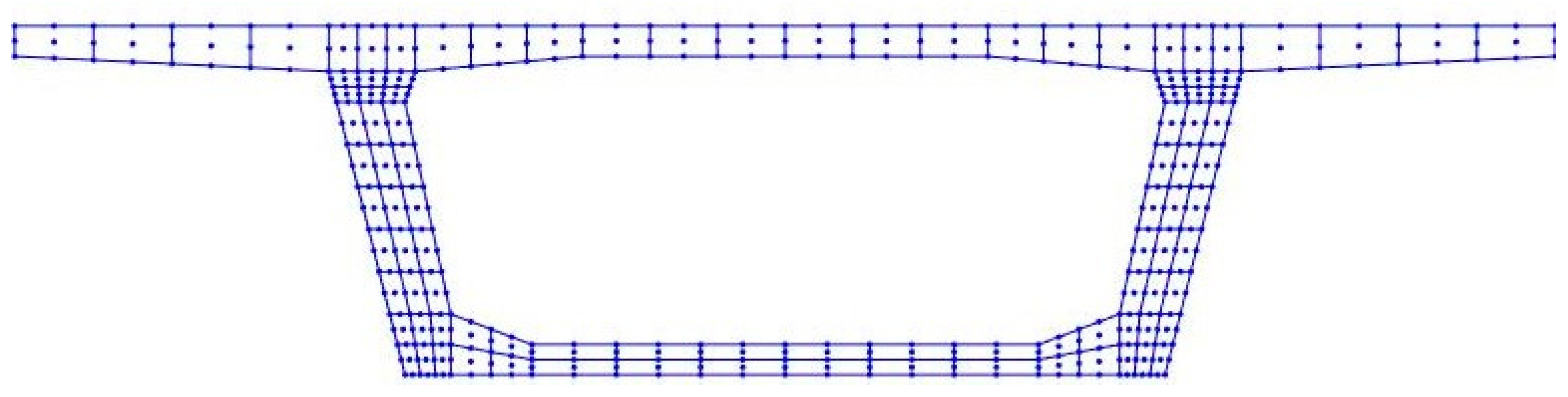
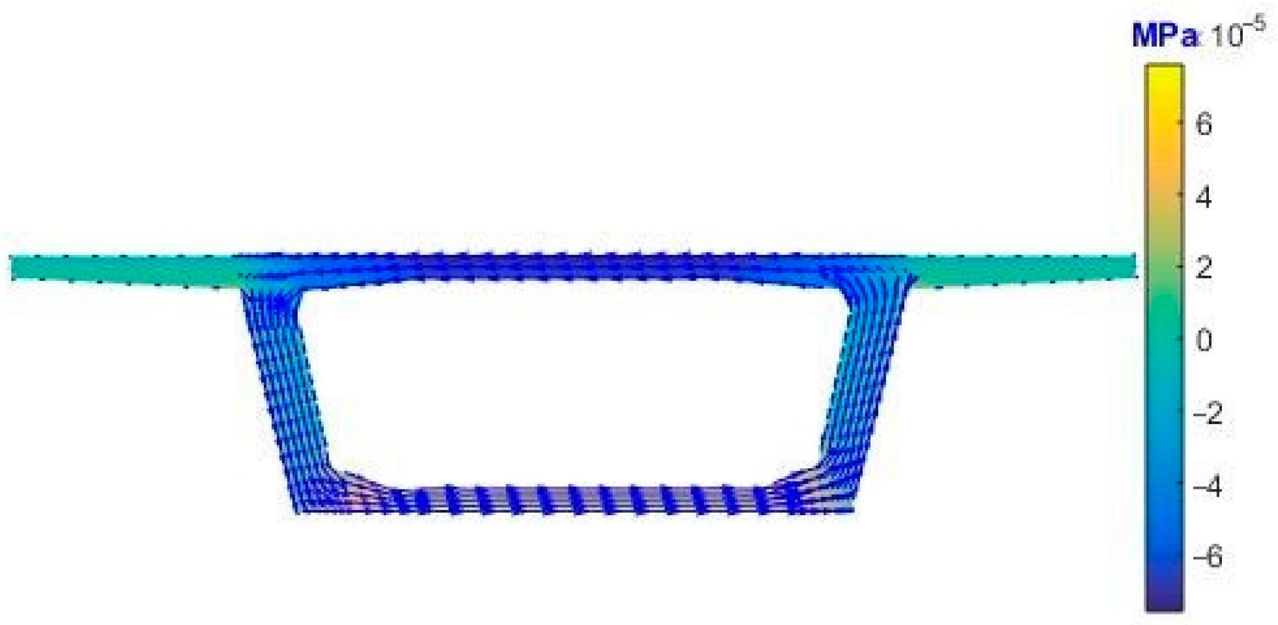
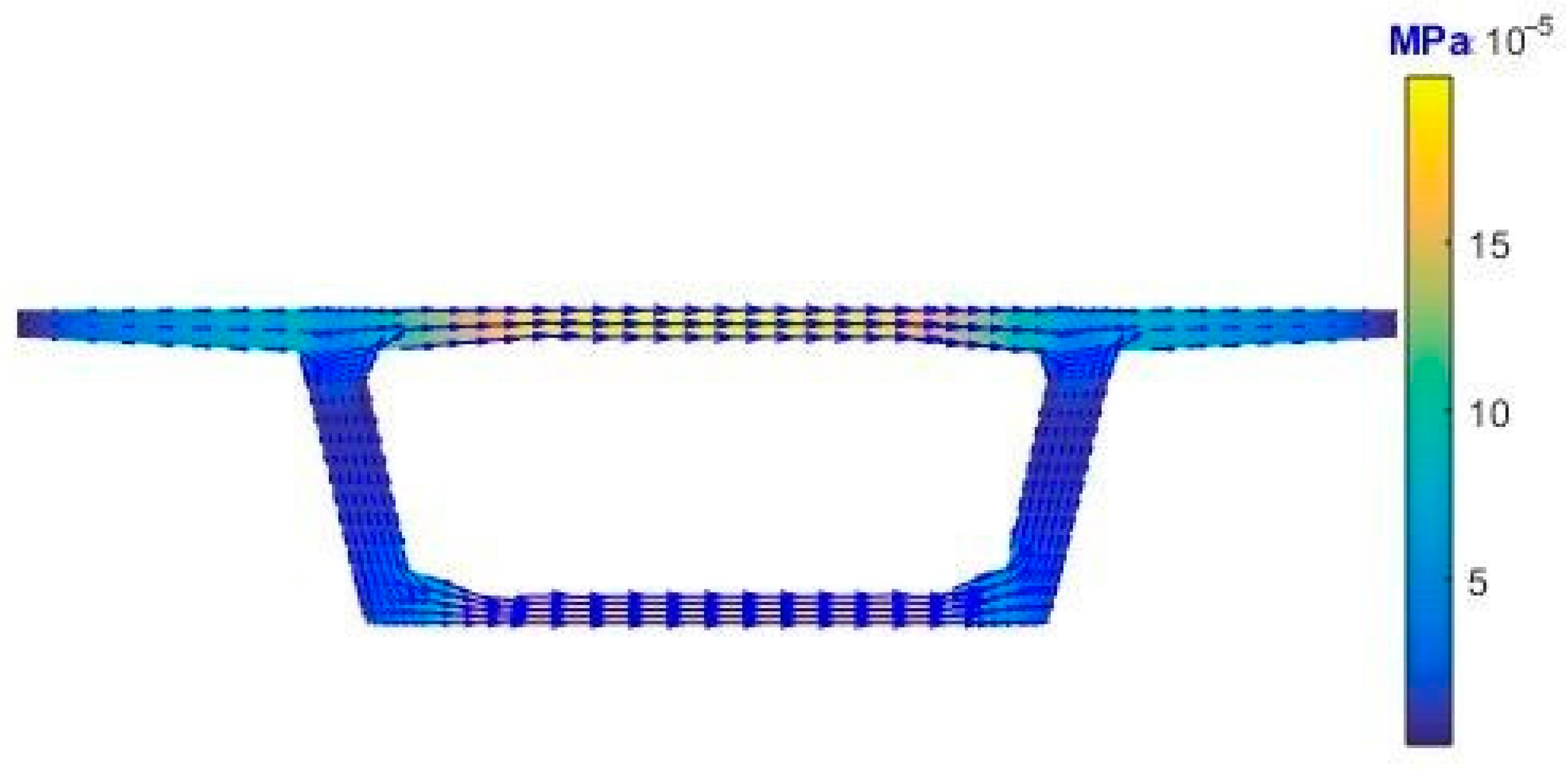
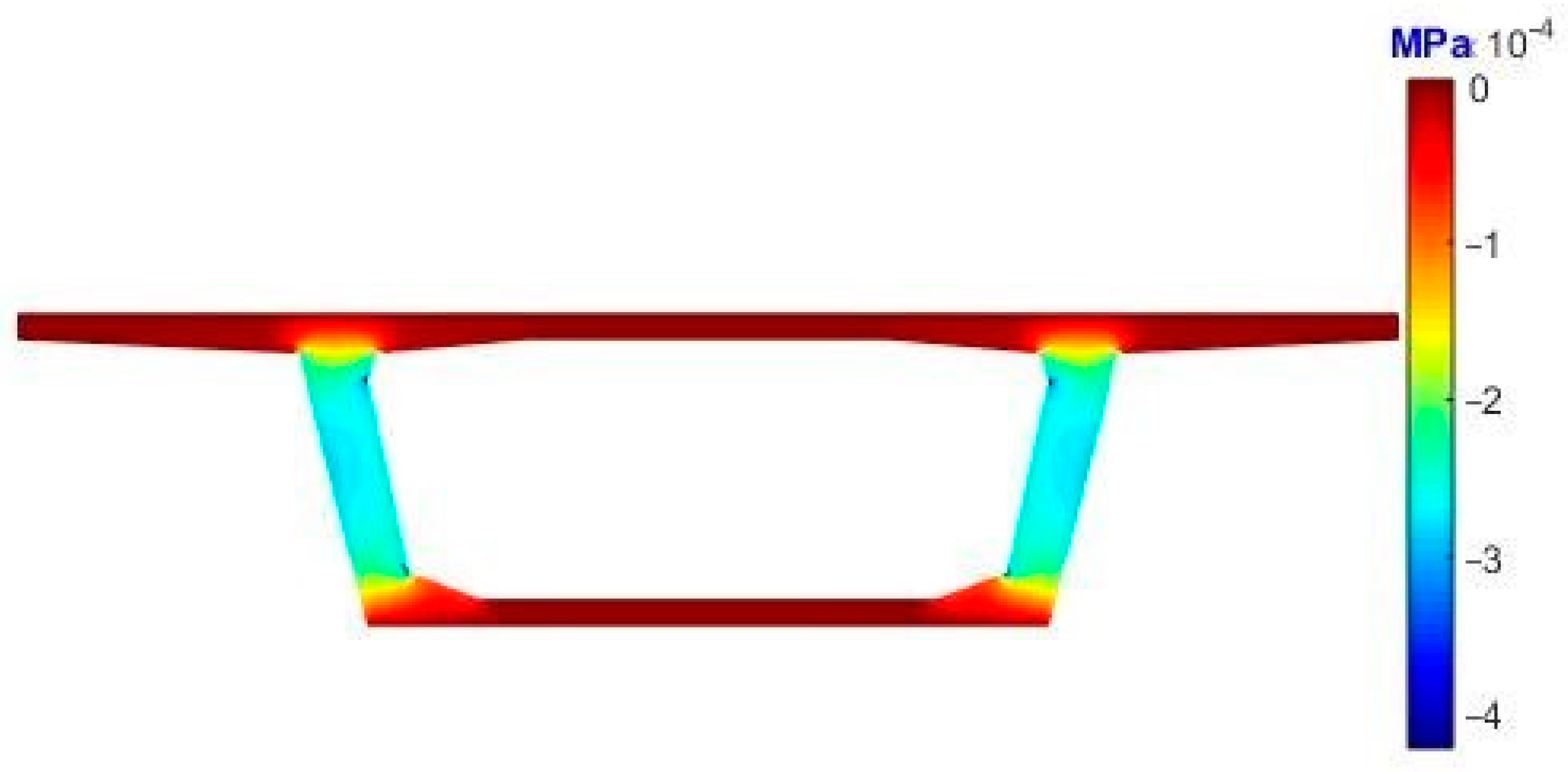
We consider the bridge cross-sections with doubly connected domain according to Figure 14. We divided the bridge cross-section into 16, 100, 1394, and 3534 elements to check the convergence of NMB and select the value to compare with FEAP. Figure 15 shows the bridge cross-section divided into 100 elements. The comparison of the polar second moment of area and the parameter $z_0$ between the two methods was performed to check the torsion problem. The resulting shear stress for the bridge-cross section under torsion $M_T=1$ [kN.m] was visualized. In the torsionless bending, the shear correction factors ${\kappa }_y{,}^{}{\kappa }_z$ and the resulting shear stress were compared between FEAP and NMB. The resulting shear stress for the bridge-cross section under shear forces $Q_y=1$ [kN], $Q_z=-1$ [kN] were also displayed. The value of the polar second moment of area and $z_0$ convergence with 3534 divided elements of bridge cross-section can be seen in

Table 12. The polar second moment of area and $z_0$ with number of elements and nodes of NMB.

Number of Elements	Number of Nodes	${\mathit{I}}_{\mathit{T}}\left[{\mathbf{m}}^4\right]$	${\mathit{z}}_0\left[\mathbf{m}\right]$
16	96	43.583	1.771
100	506	43.3162	1.773
1394	6028	43.2953	1.773
3534	14,948	43.2941	1.773

. In

Table 13. The polar second moment of area and $z_0$ parameter.

Factors	FEAP [3]	NMB	Error, %
$I_T$ [m4]	42.487	43.2941	1.89
$z_0$ [m]	1.775	1.773	0.112

, we present a comparison of the polar second moment of area and the parameter $z_0$ between NMB with FEAP. The error is under 1.89%. Fifty thousand nodes and uniform mesh were used to achieve the convergence results when using FEAP. The error of the convergence is 0.0047% [3]. Meanwhile, NMB is convergent with 14,948 nodes. The error of the convergence is 0.0027%, see Table 12. This result shows that the computation speed of NMB is faster and more efficient than FEAP.

Figure 16 depicts the distribution of shear stress ${\tau }_{xy}$ and the resulting shear stresses of the bridge cross-section under torsion $M_T=1$ [kN.m] of NMB. The maximum shear stress ${\tau }_{xy}$ is $7.59\times {10}^{-2}$ [kPa].

Figure 17 shows the distribution of shear stress ${\tau }_{xy}$ and the resulting shear stresses due to $Q_y=1$ [kN]. The maximum shear stress ${\tau }_{xy}$ is $2.05\times {10}^{-1}$ [kPa]. Figure 18 displays the distribution of shear stress ${\tau }_{xz}$ induced by $Q_z=-1$ [kN]. The maximum shear stress ${\tau }_{xz}$ of NMB and SCAD [7,8] is $4.15\times {10}^{-1}$ [kPa] and $4.03\times {10}^{-1}$ [kPa], respectively.

Table 14. Shear correction factors ${\kappa }_y,{\kappa }_z$ with $\nu =0$.

Factors	FEAP [4]	NMB	Error, %
${\kappa }_y$	0.5993	0.587293	2.00
${\kappa }_z$	0.2311	0.238114	3.04

and

Table 15. Shear correction factors ${\kappa }_y$, ${\kappa }_z$ with $\nu =0.2$.

Factors	FEAP [4]	NMB	Error, %
${\kappa }_y$	0.5993	0.587292	2.00
${\kappa }_z$	0.2312	0.238114	2.99

show the errors of the shear correction factors between FEAP and NMB are under 3.04%.

3.5. Bridge Cross-Section with Multiply Connected Domains

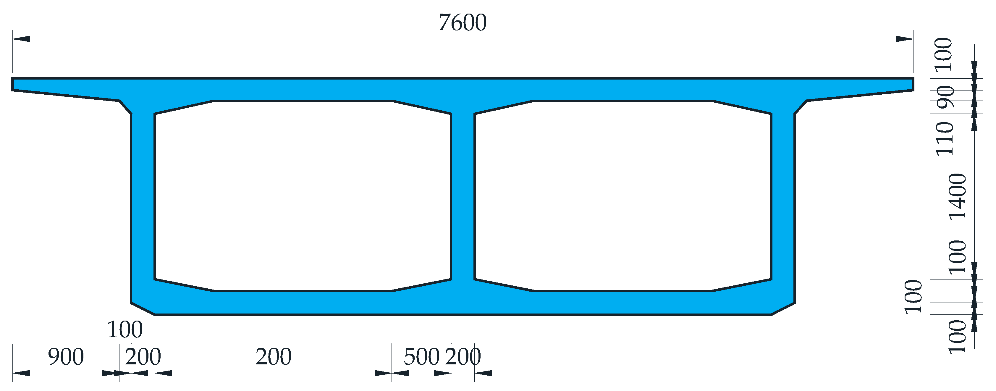
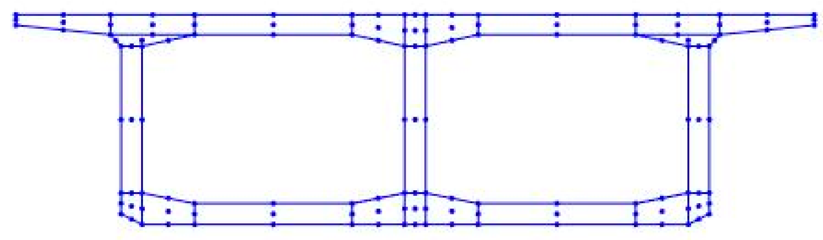
As a final example, we examined the bridge cross-section with multiply connected domains according to Figure 19 [7]. Poisson’s ratio is taken as $\nu =0.2$. The comparison between NMB and SCAD [7,8] was performed. Figure 20 depicts the bridge cross-section divided into 23 elements.

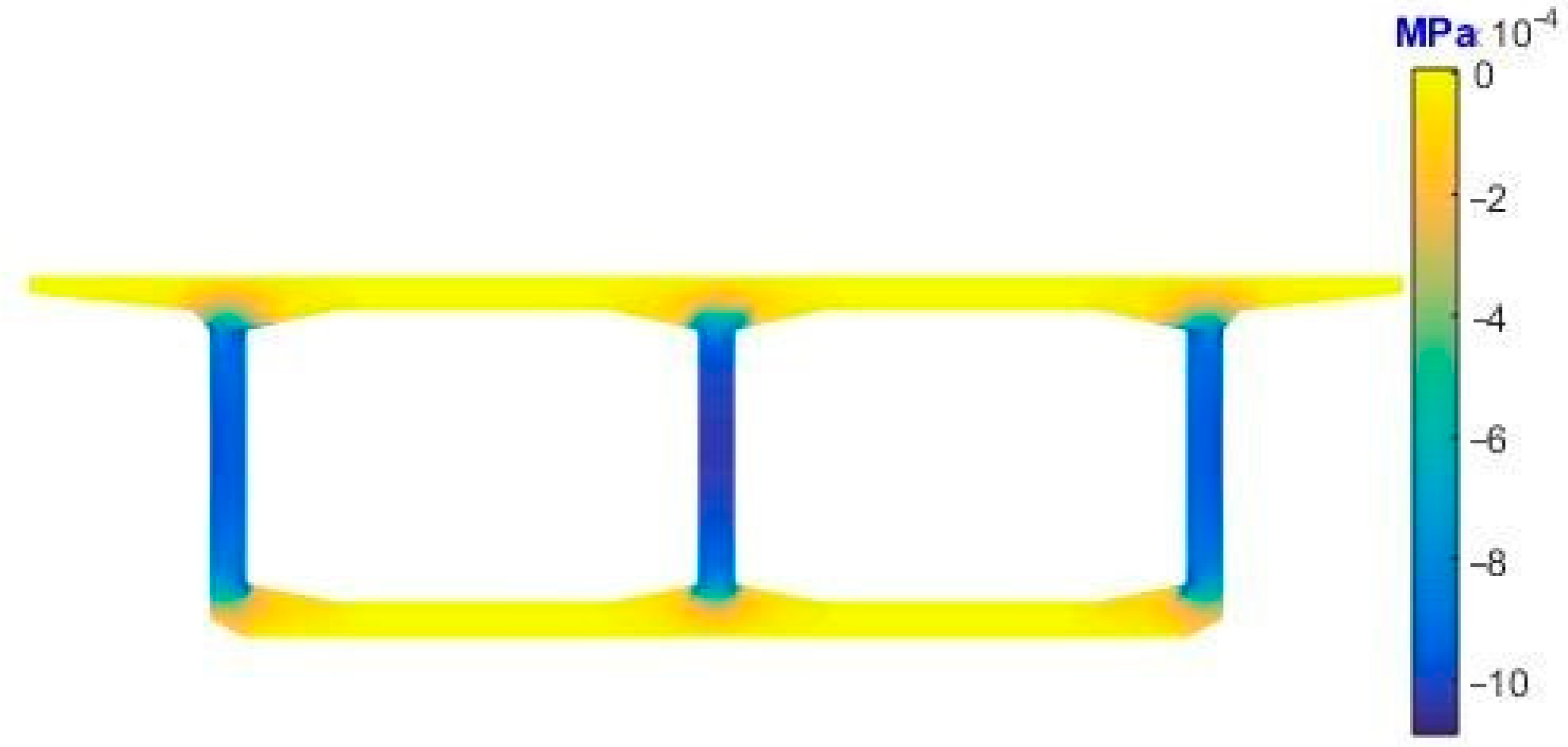
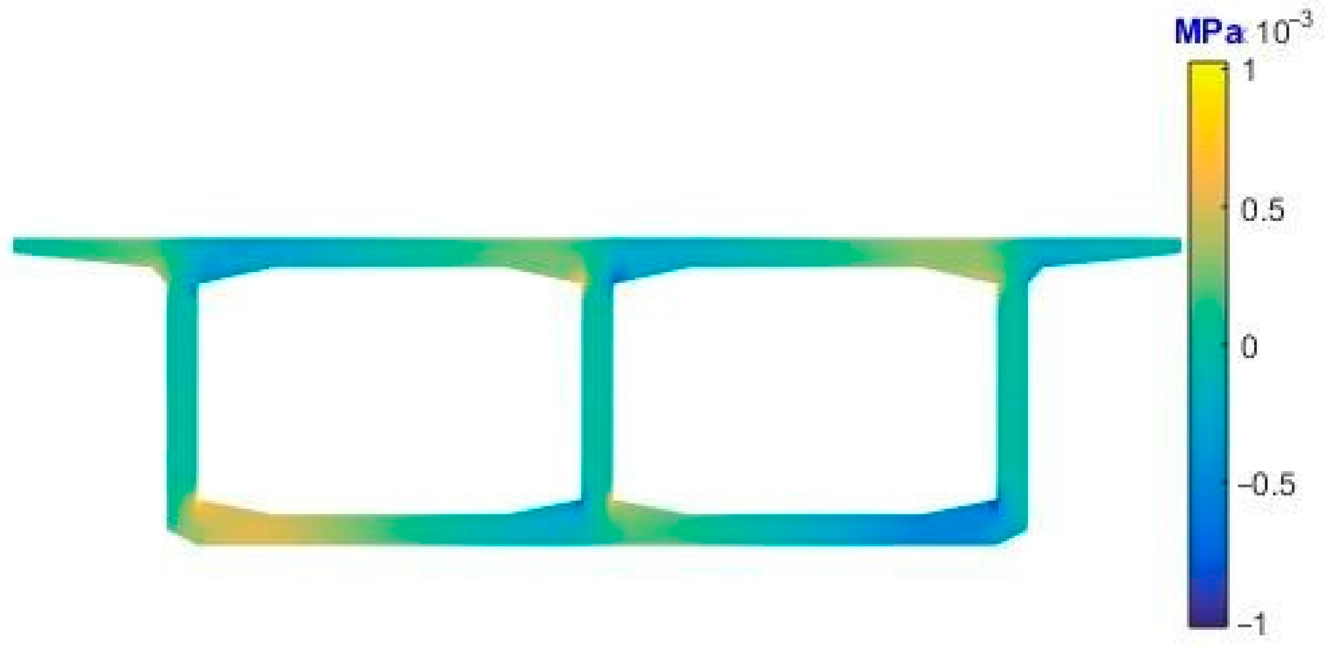
Figure 21 shows the distribution of shear stress ${\tau }_{xz}$ and the resulting shear stress due to $Q_z=-1$ [kN]. The maximum shear stress ${\tau }_{xz}$ of NMB and SCAD [7,8] is the same value: 1.08 [kPa]. Figure 22 depicts the distribution of shear stress ${\tau }_{xy}$ induced by $Q_z=-1$ [kN]. The maximum shear stress ${\tau }_{xy}$ of NMB and SCAD [7,8] is 1.02 [kPa] and 0.96 [kPa], respectively.

Table 16. The shear stress ${\tau }_{xz}$ due to $Q_z=-1$ [kN], the polar second moment of area, and the shear correction factors ${\kappa }_y$, ${\kappa }_z$.

Factors	SCAD [7,8]			NMB
	539 Nodes	1817 Nodes	6857 Nodes	135 Nodes	2593 Nodes
$\max \left|{\tau }_{xz}\right|$ [kPa]	1.00	1.04	1.08	0.994	1.08
$I_T$ [m4]	5.67	5.74	5.77	5.74	5.70
${\kappa }_y$	0.655	0.647	0.644	0.649	0.646
${\kappa }_z$	0.276	0.268	0.266	0.274	0.268

shows a comparison between SCAD and NMB. It is clear from Table 16 that even when the mesh is not smooth enough (23 elements, 135 nodes), NMB still gives the same results as SCAD using 539 nodes. When using NMB, 2593 nodes (570 elements) are necessary for convergence, while SCAD is 6857 nodes.

4. Conclusions

From Gruttmann’s articles [3,4], we developed the numerical method (NMB) by using nine-noded quadrilateral elements to solve the shear stress for the prismatic beam with arbitrary cross-section. The verification of NMB was carried out by analyzing five examples.

The first example was a simple rectangle cross-section. The comparison results show a good agreement between NMB and FEAP. The second example with varying width cross-section also shows the harmony of NMB and FEAP. However, NMB used a lower number of nodes to achieve the convergence of the problem. The third and fourth examples clearly demonstrate the efficiency of using NMB to achieve convergence results. The fifth example comparing NMB with SCAD commercial software made the advantages of NMB clear.

In this paper, the shear stress problem is solved just for a single material. As a line of further investigation, we intend to extend it to different materials. The study has shown the efficiency and reliability of the method, which allows for more precise analysis and design of cross-sections. Therefore, the development of the method helps engineers to dare to design large span slender structures with reduced dimensions that are also safe. Significant savings of material will have a positive impact on carbon footprint and will enable the sustainable development of humankind.

References

- Collins, M.P.; Bentz, E.C.; Sherwood, E.G.; Xie, L. An adequate theory for the shear strength of reinforced concrete structures. Mag. Concr. Res. 2008, 60, 635–650. [Google Scholar] [CrossRef] [Green Version]
- Sung, Y.C.; Chang, D.W.; Cheng, M.Y.; Chang, T.L.; Liu, K.Y. Enhancing the structural longevity of the bridges with insufficient seismic capacity by retrofitting. Struct. Longev. 2009, 1, 1–16. [Google Scholar]
- Gruttmann, F.; Sauer, R.; Wagner, W. Shear stresses in prismatic beams with arbitrary cross-sections. Int. J. Numer. Methods Eng. 1999, 45, 865–889. [Google Scholar] [CrossRef]
- Gruttmann, F.; Wagner, W. Shear correction factors in Timoshenko’s beam theory for arbitrary shaped cross-sections. Comput. Mech. 2001, 27, 199–207. [Google Scholar] [CrossRef] [Green Version]
- Taylor, R.L. FEAP-A Finite Element Analysis Program; University of California: Berkeley, CA, USA, 2014. [Google Scholar]
- FEAP. 2020. Available online: http://projects.ce.berkeley.edu/feap/ (accessed on 17 November 2020).
- Fialko, S.Y.; Lumelskyy, D.E. On numerical realization of the problem of torsion and bending of prismatic bars of arbitrary cross section. J. Math. Sci. 2013, 192, 664–681. [Google Scholar] [CrossRef]
- Scadsoft. Available online: https://scadsoft.com/en (accessed on 17 November 2020).
- Garcia, J.M.B.; Bernat, A.R.M. Coupled model for the non-linear analysis of anisotropic sections subjected to general 3D loading. Part 1: Theoretical formulation. Comput. Struct. 2006, 84, 2254–2263. [Google Scholar] [CrossRef]
- Garcia, J.M.B.; Bernat, A.R.M. Coupled model for the nonlinear analysis of sections made of anisotropic materials, subjected to general 3D loading. Part 2: Implementation and validation. Comput. Struct. 2006, 84, 2264–2276. [Google Scholar] [CrossRef]
- Poliotti, M.; Jesús-Miguel, B. B-spline sectional model for general 3D effects in reinforced concrete elements. Eng. Struct. 2020, 207, 110200. [Google Scholar] [CrossRef]
- Yoon, K.; Lee, P.-S. Modeling the warping displacements for discontinuously varying arbitrary cross-section beams. Comput. Struct. 2014, 131, 56–69. [Google Scholar] [CrossRef]
- Navrátil, J.; Michalčík, L.; Kabeláč, J. Praktické Dimenzování Železobetonových a Předpjatých Průřezů Při interakci Vnitřních Sil, Sborník Příspěvků 22; Mezinárodní Sympozium Mosty/Bridges 2017: Brno, Czech Republic, 2017; pp. 177–183. ISBN 978-80-86604-71-8. [Google Scholar]
- Genoese, A.; Genoese, A.; Bilotta, A.; Garcea, G. A mixed beam model with non-uniform warpings derived from the Saint Venànt rod. Comput. Struct. 2013, 121, 87–98. [Google Scholar] [CrossRef]
- Jog, C.S.; Imrankhan, S.M. A finite element method for the Saint-Venant torsion and bending problems for prismatic beams. Comput. Struct. 2014, 135, 62–72. [Google Scholar] [CrossRef]
- Urbański, A. Analysis of a beam cross-section under coupled actions including transversal shear. Int. J. Solids Struct. 2015, 71, 291–307. [Google Scholar] [CrossRef]
- Beheshti, A. A numerical analysis of Saint-Venant torsion in strain-gradient bars. Eur. J. Mech. A Solids 2018, 70, 181–190. [Google Scholar] [CrossRef]
- Sapountzakis, E.J.; Tsiptsis, I.N. Quadratic B-splines in the analog equation method for the nonuniform torsional problem of bars. Acta Mech. 2014, 225, 3511–3534. [Google Scholar] [CrossRef]
- Sapountzakis, E.J.; Protonotariou, V.M. A displacement solution for transverse shear loading of beams using the boundary element method. Comput. Struct. 2008, 86, 771–779. [Google Scholar] [CrossRef]
- Barone, G.; Iacono, F.L.; Navarra, G. Complex potential by hydrodynamic analogy for the determination of flexure–torsion induced stresses in De Saint Venant beams with boundary singularities. Eng. Anal. Bound. Elem. 2013, 37, 1632–1641. [Google Scholar] [CrossRef] [Green Version]
- Paradiso, M.; Vaiana, N.; Sessa, S.; Marmo, F.; Rosati, L. A BEM approach to the evaluation of warping functions in the Saint Venant theory. Eng. Anal. Bound. Elem. 2020, 113, 359–371. [Google Scholar] [CrossRef]
- Di Paola, M.; Antonina, P.; Roberta, S. De Saint-Venant flexure-torsion problem handled by Line Element-less Method (LEM). Acta Mech. 2011, 217, 101–118. [Google Scholar] [CrossRef] [Green Version]
- Allplan Bridge Features. Available online: https://www.allplan.com/products/allplan-bridge-2019-features/ (accessed on 27 December 2020).
- Timoshenko, S.; Timoshenko, S.; Goodier, J.N. Theory of Elasticity; Timoshenko, S., Goodier, J.N., Eds.; McGraw-Hill Book Company: New York, NY, USA, 1951. [Google Scholar]
- Pilkey, W.D. Analysis and Design of Elastic Beams: Computational Methods; John Wiley & Sons: Hoboken, NJ, USA, 2002. [Google Scholar]
- Zienkiewicz, O.C.; Taylor, R.L.; Zhu, J.Z. The Finite Element Method: Its Basis and Fundamentals; Elsevier: Amsterdam, The Netherlands, 2005. [Google Scholar]
- Reddaiah, P. Deriving shape functions for 9-noded rectangular element by using lagrange functions in natural coordinate system and verified. Int. J. Math. Trends Technol. (IJMTT) 2017, 51, 6. [Google Scholar]
- SAP2000. Available online: https://www.csiamerica.com/products/sap2000 (accessed on 17 November 2020).
- Čermák, M.; Sysala, S.; Valdman, J. Efficient and flexible MATLAB implementation of 2D and 3D elastoplastic problems. Appl. Math. Comput. 2019, 355, 595–614. [Google Scholar] [CrossRef] [Green Version]
Figure 1.
(a) Shear failure of Air Force Warehouse beams [1]. (b) Shear failure of pier wall of the Wu-Shi Bridge in the Chi-Chi earthquake [2].
Figure 2.
Cross-section of a prismatic bar.
Figure 3.
Nine-noded isoparametric quadrilateral element.
Figure 4.
Computed shear stresses (a) and (b) for square section of the numerical method (NMB).
Figure 5.
Normalized shear stress for a square-cross section of NMB with (a) and (b) v = 0.25.
Figure 6.
The dimension of cross-section with varying width in mm.
Figure 7.
The cross-section divided into 48 elements.
Figure 8.
Shear stress and resulting shear stresses for due to [kN].
Figure 9.
The dimension of cross-section of crane rail A100 in mm.
Figure 10.
The discretization of cross-section by (a) FEAP and (b) NMB.
Figure 11.
Shear stress and resulting shear stresses due to [kN.m].
Figure 12.
Figure 13.
Figure 14.
Bridge cross-section with dimensions in mm.
Figure 15.
The bridge cross-section divided into 100 elements.
Figure 16.
Shear stress and resulting shear stresses due to [kN.m] by NMB.
Figure 17.
Shear stress and resulting shear stresses due to [kN] by NMB.
Figure 18.
Shear stress due to [kN] by NMB.
Figure 19.
Figure 20.
The bridge cross-section divided into 23 elements.
Figure 21.
Figure 22.