Developing a Parametric Cash Flow Forecasting Model for Complex Infrastructure Projects: A Comparative Study

Abstract

Forecasting the cash flow for infrastructure projects has not received much attention in the existing models. Moreover, disregarding the cost flow behaviour and proposing models that entail a relatively high dimensionality of inputs have been the main drawbacks of the existing models. This study proposes a heuristic cash flow forecasting (CFF) model for infrastructure projects, and it explores the underlying behaviour of the cost flow. The proposed model was validated by adopting a case study approach,the actual cost flow datasets were mined from a verified data system. The results invalidated the employment of a dominant heuristic rule with regard to a cost-flow-time relationship in infrastructure projects. On the other hand, a mathematical parameter-based comparison between the trends analysed from previous studies revealed that the cost flows of infrastructure projects procured through a design-bid-build (D-B-B) route behaved in a similar manner to building projects procured through a construction management route. This research contributes to the body of knowledge providing a method to enable infrastructure contractors to accurately forecast the required working capital through adding a new dimension for project classification by coining the term “the quaternary flow percentage”. In addition, this study indicates the importance of identifying the impact of root risks on the individual cost flow components rather than on the aggregated cost flow, which is a recommendation for future research.

1. Introduction

In the construction industry, cash flow has been recognized as a serious issue that adversely affects the performance of contracting organizations for decades, according to [1,2]. From a contractor’s perspective, the cash flow forecasting (CFF) process is concerned with periodically predicting the cash outflow (i.e., cost) and the cash inflow (i.e., revenue) to determine the net cash flow profile (i.e., the variance between the inflow and outflow) [3]. A positive net cash flow indicates that the project is able to finance itself, whereas a negative net cash flow indicates that working capital from outside a project is required [4]. Hence, it is critical for a contracting organization to forecast the working capital for a given project at the tendering stage, as well as during the construction stage, to ensure the financial functionality at the strategic level [5] (p. 232).

Accurate cash flow forecasting plays a vital role in driving economic and social sustainability in construction [6]. In terms of economic sustainability, a CFF model is keenly required to provide insights on the availability of cash inflow and cash outflow at a particular point in time. This is to avoid late payments to the supply chain and ensure cash flow circulation within the wider economy. Furthermore, late payments cause insolvency and bankruptcy in the supply chain, which result in adverse social impacts on the supply chain and the wider market. This leads to deterioration of the project’s social sustainability, which could be irreparable in the short-term. Hence, proposing a simple yet a reliable CFF model to the infrastructure industry contributes to strengthening its economic and social sustainability. In the context of contracting organizations, cash inflow is generated from the periodic payments received from the clients against the works carried out by the contractor, whereas the cash outflow is formed by applying time lags to the individual cost flows. The total cost flow is composed of summing the individual direct cost of the various resources (i.e., manpower, equipment, materials, and subcontractors) allocated to accomplish the works and the indirect costs, such as site and head office overheads [7]. Therefore, to create a very accurate cash flow profile, the cost flows of the proposed works must first be accurately forecast [8].

Heuristics are rules of thumb developed based on scientific principles. Heuristics have the benefits of being simple to understand, easy to apply, and very inexpensive to use in computer programs [9]. Developing parametric-based heuristics has become a modern trend that entails the derivation of finite parameters for a given function based on real-world scenarios to enable the prospective application of a proposed heuristic within similar environments [10] (p. 107). According to Taleb [11], the parameters of forecasting heuristics must be derived from existing cases representing the necessary information to enable a heuristic forecasting model to be reliable.

There is a current trend to develop heuristics in the field of construction management [12]. For instance, Gajpal and Elazouni [4] developed a heuristic model for contractors to optimize their cash flows by considering the financial constraints, whereas Chiu and Tsai [13] developed a priority-based heuristic rule to maximize the net cash flow with an emphasis on the constraints of resources in the project schedule. On the other hand, Boussabaine and Elhag [14] employed a heuristic in their proposed fuzzy logic technique-based cash-flow forecasting model.

Within contracting organizations, financial decisionmakers are required to infer in regard to forecasting and securing working capital for new projects at the tender stage as well as upon the award of a contract. When a probable deficit signal is flagged based on the forecast, decisions may be made to apply for short-term loans to avoid financial difficulties during the projects. However, those decisions may be questioned by the shareholders or owners, often due to optimism bias [15]. Therefore, there is no better convincing mechanism that results in their decisions being defensible than having a reliable heuristic, accompanied by its underlying patterns, that has stemmed from the context (i.e., the prevailing characteristics of the organization) for which a prospective decision is required. Thus, to develop a heuristic CFF model for contracting organizations undertaking construction projects, the actual cost flow datasets from completed projects are required. Subsequently, a model can be constructed and used as a class reference to forecast the net cash flows for future projects [16].

In view of the foregoing introduction, the aim of this study is to propose a parametric-based heuristic net CFF model constructed based on the forecasting of individual cost flows for infrastructure projects. Therefore, this study has two objectives, as follows:

• To explore the underlying behaviour of the cost flow at both the project (i.e., macro) and at the individual level of the cost component and work package (i.e., micro); and
• To develop a heuristic cost flow characterization zoning-based chart to enable a common platform for exchanging and comparing cost-flow data.

Thus, this study combines the underlying behaviour of cost flow with the proposed net CFF model constructed based on cost flow forecasts for the individual cost components. This is achieved by deriving parameters from the logit transformation technique and adopting a case study approach. The performance of the proposed model is demonstrated through an illustrative example using cost datasets of the same project and, subsequently, validated using the datasets of another infrastructure project.

2. Conceptual Background

This section reviews the relevant available studies,and identifies the research gap as well as demonstrates the importance of this study from a contractor’s perspective.

2.1. Related Work

This subsection critically reviews and classifies the available studies into three approaches.

2.1.1. Cash Flow Forecasting Using Mathematical Techniques

Proposing a net cash flow forecasting (CFF) model relying upon the cost flow curves instead of employing the value curves approach has yielded promising results [17]. The reason that the latter demonstrated unreliable and incorrect outputs was attributed to unbalanced techniques and errors in estimation. Blyth and Kaka [18] developed a CFF model using regression modelling along with the logit transformation technique to assist contractors in predicting the cost flows for building projects, while stressing the need for a more specific classification of projects for the purpose of obtaining more accurate forecasts. In contrast, Liang, et al. [19] proposed a cash flow model using derived parameters to provide clients with an expenditure forecast tool for transportation design-build projects. In studying the effects of various different procurement routes on the accuracy of cash flow forecasts, Kaka and Khosrowshahi [20] concluded that building projects procured through management contracts tended to have a slower cost flow at the initial stage compared to building projects procured through traditional contracts because the initial stage in the former was allocated to planning and subcontractor procurement.

Additionally, Khosrowshahi and Kaka [21] proposed a visual model for cash flow forecasting at the project level. This had the capability to generate a forecast from analytical analysis of the data with the application of the tacit knowledge of the user. However, it required a series of mathematical variables as inputs and did not reach down to the individual cost component levels. Considering the various cost components for a construction project, Park, et al. [22] presented a CFF model by dividing the cost of the project into manpower, material, equipment, subcontract, and indirect costs. This concept was adopted to simulate realistic behaviours/patterns of the cost flow and outflow curves so that an accurate CFF could be generated. However, the authors stressed the fact that the use of the model is dependent on a detailed schedule of the construction activities to enable an accurate forecast of the resources’ costs and the revenue, which is an intensive process.

Lucko [8] and Su and Lucko [23] went beyond the prevailing techniques by introducing the use of singularity functions, which had been traditionally used in structural element analysis, into the domain of cash flow forecasting with the aim of understanding the underlying behaviour of the cash flows. However, the implementation of the proposed methodology required detailed information on the work items involved to complete a given project, thus leading to its inapplicability within contracting organizations. In the context of the UAE, a study conducted by [24] that aimed to investigate the impact of negative cash flow trends on construction performance of building projects revealed that the deficit covered 30–70% of a given project duration and was most likely to take place after 50% of the project duration has elapsed. However, the cost flow was not categorized to its components (manpower, equipment, and materials), and it dealt with building projects only.

2.1.2. Cash Flow Forecasting Using Artificial Intelligence (AI)

Having employed heuristics with deep learning techniques to presumably enhance the accuracy of CFF models in building projects, Cheng, et al. [25] proposed a model that relies on independent and time-dependent variables. The independent input variables that express complexity of the projects are number of floors, contract cost, floor area, and duration of the project. Based on statistical performance measures, their study argues that the proposed model to be the greatest prediction model in forecasting future cash flow of construction projects. Boussabaine and Kaka [26] concluded that the cost curves generated by AI technique could be used as a proactive approach to demonstrate the direction of the cost flow of a given project. In the same vein of AI, Boussabaine and Elhag [14] proposed a framework for predicting a cash flow value at any particular period during the project’s progress based on a fuzzy logic technique using a heuristic. The heuristic assumed that at 33.33% of the contract duration, the total cost flow is at 25%, whereas at 66.66% of the contract duration, the total cost flow reaches 75%, and at the completion of the contract duration, the total cost flow is 100%.

From a practical perspective, the AI-based CFF models presented turned out to be complex due to the complication of setting up AI technology in projects. Moreover, a common criticism of using AI for solving real-world problems results from the large amounts of data required for training the models [27].

2.1.3. Cash Flow Forecasting Using Building Information Modelling (BIM)

Building Information Modelling (BIM) facilitates the quantification of unit costs incurred from the various cost components [28]. Kim and Grobler [29] and Lu, et al. [30] proposed a novel model that was capable of predicting the periods at which external finance injections would be required. However, for the two studies in the BIM context, the reliability of the models’ outputs depended on the accuracy of the schedule and the inclusion of all the building elements; additionally, both reported that intensive work was required for the inputs.

Unlike the previous BIM-based CFF models presented, Elghaish, et al. [7] developed a novel CFF framework for projects procured through the integrated project delivery (IPD) approach. The framework integrated the schedule dimension (4D) with the cost dimension (5D) BIM to generate the project cash flow. The novelty of this framework stems from its capability to notify a contractor of the maximum and minimum cash flow forecast taking into consideration the direct and indirect costs. Thus, enabling a contractor to reallocate its indirect resources to other projects in order to avoid a negative cash flow state.

In summary, the literature review reveals that various sophisticated approaches have been employed to propose CFF models, as summarised in

Table 1. Summary of literature review.

Reference	Focus of Study	Methods	Limitations
[18]	Forecasting expenditure cash flow for transportation design-build projects from clients’ perspective.	Case-based reasoning framework based on data mining of completed projects.	Limited to clients and mathematically complex.
[17]	Forecasting cumulative and monthly cost flows for building projects from contractors’ perspective.	Regression modelling and logit transformation techniques were employed.	Limited to building projects and required numerous inputs.
[24]	Forecasting cash flow (inflow) for building projects from contractors’ perspective.	Integration of meta- heuristic with artificial neural network.	Limited to building projects, neglected the outflow, and complicated implementation.
[6]	Generating cash flow curves for projects procured through integrated project delivery (IPD) approach.	Integration of 4D BIM with 5D BIM.	Limited to IPD building projects.

.

2.2. Research Gap and Motivation

Despite the established importance of infrastructure projects, forecasting the cost/cash flow thereof, from a contractor’s perspective, has not received sufficient attention in the existing CFF models. Furthermore, a reliable yet simple CFF model does not exist for infrastructure projects, in particular, within the context of the United Arab Emirates (UAE). On the other hand, the consideration taken to treat various projects as identical in terms of the cost flow behaviour is a main drawback of the existing CFF models. For instance, commercial projects exhibit different cost flow patterns than infrastructure projects owing to the dissimilar characteristics governing their environmental and situational contexts.

Hence, there has been a void in the literature with regard to the characterization of the cost flow behaviour, thus resulting in the unreliability of the proposed CFF models, as the underlying foundation (i.e., the embedded behaviour of the data) used to construct those CFF models has not been visible (i.e., vague). As such, it is contended that the characterization of the cost flow needs to be included in a forecasting model to qualify it for practical implementation, which is the overarching motivation behind this study.

3. Research Methodology

This section reports the research strategy and approach adopted for the data collection. It also outlines the methods employed for data analysis purposes, and the statistical/mathematical equations that are used to perform the analysis and construct the CFF model.

3.1. Research Strategy

Case-based research enables the generation of in-depth knowledge of a given phenomenon and the determination of its patterns, according to [12,31]. In a similar vein, Koskela [32] and Talebi [33] urged scholars in the domain of construction management to produce relevant research through real cases by reaching the root causes of identified problems instead of relying upon imaginary cases and jumping directly to solutions that may contribute nothing to the construction management field. There exist two main types of case studies, i.e., single case studies and multiple case studies [34] (p. 38). In this regard, Yin [34] (p. 39) states that a single case study is often used because it provides an opportunity to observe and to analyse a phenomenon that few have considered before to define the actual case; additionally, it enables the researcher to challenge an existing theory and to provide a source of new research questions using multiple units of analysis, that is, considering various embedded factors. On the other hand, multiple case studies are often adopted with a single unit of analysis to arrive at holistic findings. Taking into consideration the strengths that the utilization of a single case study approach provides, this approach has been selected for the present study. This is because the present study aims at investigating the cost flows behaviour of infrastructure projects prior to the employment of the dataset in the process of building the proposed CFF model, along with the provision of a detailed explanation of the identified patterns. As such, a single case study approach as the research strategy representing infrastructure projects in the UAE is warranted to accomplish the research objectives. In this regard, one completed infrastructure project in the UAE has been chosen to serve as the case study to investigate the underlying behaviour of the cost flows at the aggregated (i.e., project and total cost) as well as at the individual (i.e., work package and the individual cost component) levels. In addition, the actual cost dataset of this project (Project 1) has been used to construct the cost/cash flow forecasting model. Subsequently, the proposed CFF model was tested and validated by comparing the forecast and actual values to those of a second infrastructure project (Project 2).

3.2. Data Collection

The objectives of this research necessitate the use of a highly detailed level of data reaching down to the resource level used to complete a specific activity under a given work package. For instance, the details of the actual resources used to substantially complete a pipeline under the sewer work package must be known to investigate the behaviour of the cost flow for this work package. Accordingly, the actual monthly cost datasets of the two completed infrastructure projects have been obtained from a leading contracting organization in the UAE that has shown interest in the research aim. The contract form adopted for both projects was a bespoke FIDIC Red Book “Conditions of Contract for Construction of Buildings and Engineering Works Designed by the Employer” [35]. The completion times, including time extensions, were 638 days and 709 days for the projects used to develop and test the model, respectively. Subsequently, the authors have validated and verified the datasets mined from a structured monitoring system implemented by the participating contracting organization.

Table 2. Summary of the scopes of work of the selected projects.

Serial Number	Work Package (Network)	Brief Description of the Scope of Work	Unit of Measurement	Quantification (Project 1, Case Study)	Quantification (Project 2, Validation Project)
1	Internal Roads	Cut/fill, pavement, kerbstone, and interlock tiles.	linear metre	9400.00	9900.00
2	Sewerage	Pipelines and manholes.	linear metre	6250.00	8500.00
3	Strom Water	Pipelines and manholes.	linear metre	12,400.00	9000.00
4	Electrical	Electrical cables and substations.	linear metre	25,000.00	37,000.00
5	Street Lighting	Electrical cables and poles.	number	210.00	240.00
6	Potable Water	Pipelines and valves.	linear metre	9750.00	9300.00
7	Telecom	Telecom ducts with joint boxes.	linear metre	25,000.00	18,000.00

demonstrates the quantification of the work packages along with brief descriptions of the scopes of work for each of the two selected projects.

Additionally,

Table 3. Proportions of the individual cost components.

Cost Component	Project 1 (Case Study) Data	Project 2 (Validation Project) Data	Data Ranges Reported by [22]
Direct Equipment	24.98%	21.91%	10% to 25%
Direct Manpower	13.19%	11.00%	5% to 15%
Direct Materials	47.22%	55.26%	25% to 35%
Indirect (i.e., preliminaries)	14.61%	11.83%	5% to 15%
Total	100.00%	100.00%	N/A

presents the proportion of each individual cost component out of the total costs for both projects. The results align with the ranges reported in [22], except for the proportion of the materials cost, which is compatible with the ranges reported by [2], who state that materials cost may amount to 50% of the total project cost.

3.3. Data Analysis

After the datasets were processed and validated, the analysis part commenced. The data analysis was conducted using the following approaches:

3.3.1. Visual Examination of the Cost Flow Curves

Visualization is one of the categories used in data mining; it is an analytical process for searching for consistent patterns in large data sets to improve the knowledge about a given phenomenon [36]. As such, this approach has been adopted to achieve the study objectives in regard to the cost flow characterization. To implement this approach, the actual monthly cost flows have been graphically drawn to arrive at visual curves for behaviour analysis purposes. Initially, this was conducted at the macro-level (i.e., project level) using the total direct and indirect costs with respect to the time in a cumulative manner. Thereafter, the periodic behaviour of the individual cost components forming the total direct cost flow was examined. At this step, an in-depth analysis was performed at various completion percentages to reveal how the cost flow behaved at different stages and which cost component dominated a given completion stage.

It is argued that using raw cost data by simple data processing and averaging at the macro-level of a given construction project probably leads to an inaccurate cost/cash flow forecasting model, as the underlying behavioural patterns at the micro-level would be unknown to the prospective user of a proposed model. Thus, the investigation of the underlying cost flow behaviour at the individual cost component as well as at the dominant work package (i.e., micro-level) levels are important in the development of a forecasting model to gain insight into the circumstances that shaped the cost flow patterns, as there was an absence of such descriptive knowledge in the literature reviewed. Unlike the surveyed studies reviewed previously, this study has dealt with the underlying behaviour of the cost flow; therefore, the analysis has been performed at the individual cost component level and at the work package level. As a result of the analyses, a cost flow characterization zoning-based chart has been proposed hereinafter.

3.3.2. Modelling the Cost Curves Using the Logit Transformation Technique

To propose a parametric-based heuristic CFF model, a statistical technique that is able to derive the parameters was required. Having investigated the previous studies (i.e., [18,27]) conducted in this domain, it was found that the logit transformation technique has gained momentum over the polynomial regression analysis technique in modelling the cash/cost flow curves owing to its simplicity, as well as to its ability to represent the S-curve in a linear form (i.e., smoothening). The simplicity is expressed by the number of the inputs, i.e., two parameters, for the logit transformation technique, whereas the regression technique entails more parameters, which leads to impracticability and exposure to more errors [5] (p. 44).

In this regard, the linear equation is found by Equation (1) for both the independent and dependent variables (in this case, time and cost), as follows:

$$Logit=ln\frac{z}{1-z}$$

(1)

where z is the variable to be transformed and Logit is the transformation. Once the two variables are transformed, a linear equation can be fitted into the transformed data. This linear equation is expressed in Equation (2) as follows:

$$Y=\alpha +\beta X$$

(2)

where:

$$Y=ln\frac{c}{1-c}$$

(3)

$$X=ln\frac{t}{1-t}$$

(4)

To transform the data for a particular project, X and Y must be calculated for each value of t (time) and c (cost), respectively. Deriving the constants α and β is, thus, a simple linear regression of the transformed data. The detailed procedure for deriving the constants α and β is outlined in [5]. Once α and β are derived, the fitted S-curve can be generated using Equation (5), as follows:

$$C=\frac{F}{1+F}$$

(5)

where:

$$F=e^{\alpha }\left(\frac{t}{1-t}\right)^\beta$$

(6)

Equation (5) then forms the equation of the sigmoid curve, which describes the cost flow of a specific project.

In the context of the goodness-of-fit for the Logit transformation technique, the following equation is used:

$$SDY=\sqrt{\frac{{\mathsf{\Sigma }\left(Y-YE\right)}^2}{\left(N-2\right)}}$$

(7)

where:

SDY is the standard deviation about the estimate of Y;

Y is the actual value at any accounting period;

YE is the estimated (or fitted) value; and

N is the number of observations (accounting periods).

Accordingly, the model with the lowest value of SDY has the best fit and, hence, is the most accurate. This allows the determination of the reliability and accuracy of the models according to [5].

Using the above technique, the Alpha and Beta parameters for each cost component were derived separately to develop the proposed model. Thereafter, the aggregated cost flow of the selected project was forecast and, subsequently, compared with the actual values.

4. Results and Discussion

This section deals with cost data analysis and the investigation of the underlying behaviour of the cost flow at both the project and work package level. Furthermore, it presents the CFF model and its parameters as well as provides a framework describing the procedural steps to implement the developed model in practice. It concludes by comparing the resultant cash flow forecast with the actual cash flow for the selected case-study projects.

4.1. The Underlying Behaviours of Cost Flows

This section presents the analyses performed on the cost flow datasets obtained from the case-study project to characterize the mechanism (behavioural patterns) of the cost flow prior to its employment in the development of the cost/cash flow forecasting model used to accomplish the objectives of the study. Towards the end of this section, a heuristic cost flow characterization chart will be presented to pave the way towards the development of a heuristic cost/cash flow forecasting model.

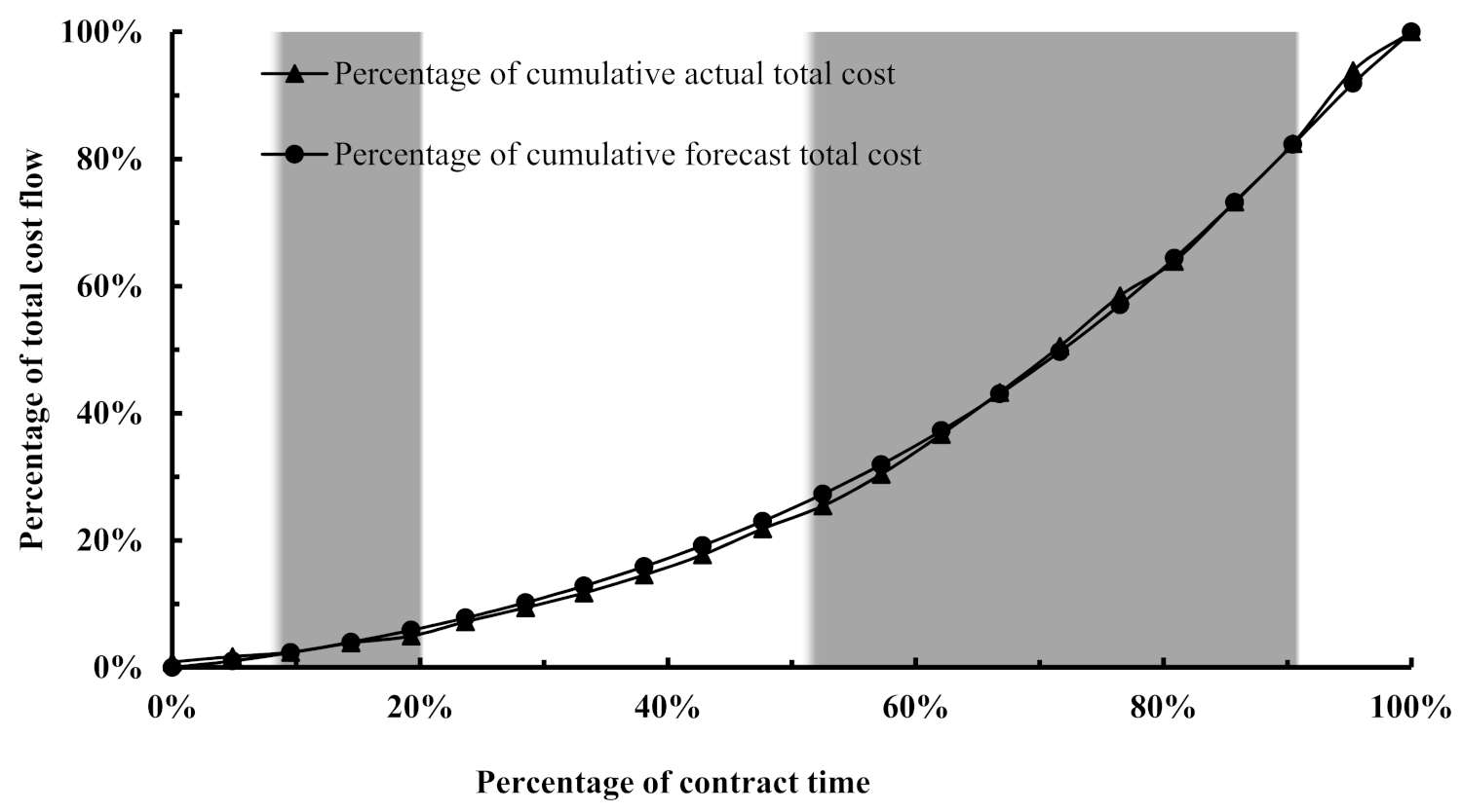
4.1.1. The Aggregated Cumulative Cost Flow Behaviour at the Project Level

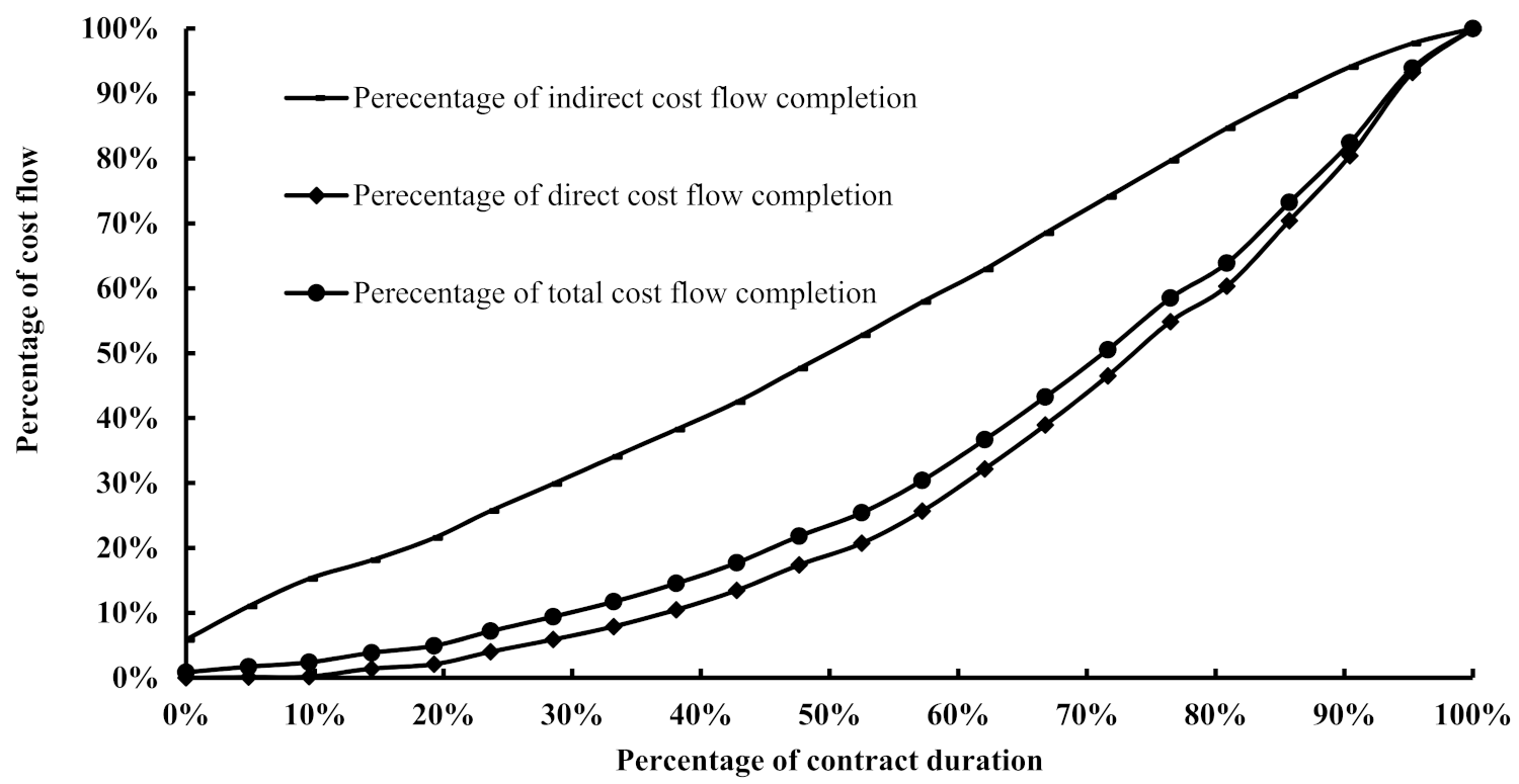
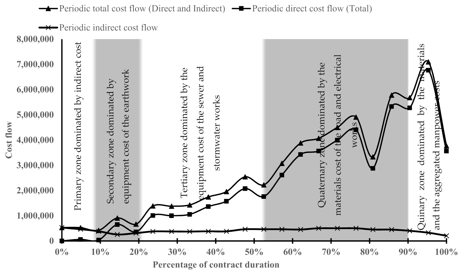
Figure 1 presents the cumulative percentage of the aggregated cost flow along with the direct and indirect cost flows against the contract duration (CD). As expected, the aggregated cost flow is a function of the direct cost flow, as the latter contributed to 85.39% of the total cost flow according to Table 3.

As shown in Figure 1, the direct cost flow started to generate/move at a growing trend when the contract duration reached 20%, whereas it was at a steady state from the beginning of the contract until that point in time. This observed slow trend of the cost flow during the initial period of infrastructure projects procured through the DBB route is ascribed to the amount of time required to complete the engineering documents (e.g., shop-drawings) as well as obtaining approvals from the statutory authorities following a thorough site survey. This survey process is an essential part to record the existing ground and network elevations to complete and coordinate the drawings of the various work packages. It is generally time consuming and may cover dozens of kilometres and hectares. However, a contractor might take risk during this period and commence with general activities, as was the case in the project studied, whereby the direct cost flow generated initially was a result of the soil improvement activities that took place in parallel to the engineering process. The observed trend of this initial slow progress in terms of the cost flow, which reflects the cash flow, is underpinned by a study conducted by [20] that indicated that the cost flows of some types of contracts, such as management contracts of building projects having a duration longer than thirteen (13) months, tend to be slow for a few months at the start of a project. They attributed this initial slow trend to the planning process and the selection of subcontractors.

Interestingly, the aggregated cost flow trend shown in Figure 1 is inconsistent with the heuristic rule cited by [14], which was referred to earlier. For instance, the cost flow percentage shown in Figure 2 at 33% of the contract duration is 12%, whereas according to [13], the cost flow percentage should typically have reached 25%. Moreover, according to them, when the project has reached 66%, the cost flow percentage has typically accumulated to 75%; however, Figure 1 reveals that at 66% of the contract duration, the total cost flow had accumulated to only 44%. This contrast in the cost flow trend has been attributed to the fact that the cited heuristic rule might have been based on projects procured through a different route than the one used in this study and may have involved one work package only, such as a water pipeline project.

4.1.2. The Periodic Cost Flow Behaviour of Individual Cost Components at the Project Level

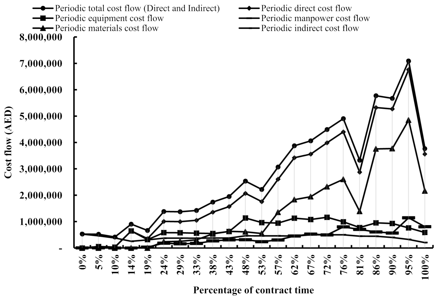
To gain insight into the behaviour of the individual cost components and the influences thereof on the aggregated cost flow, the cost datasets have been plotted in a periodic manner, as depicted in Figure 2. The periodic trends offer an explanation of and are able to characterize the underlying patterns of the cost flow since the periodic changes can be traced by visual inspection of the cost flow profiles [37].

A first glance at Figure 2 reveals that the total cost flow curve during the first 10% of the contract duration was a function of the indirect cost flow resulting from the insurance and mobilization costs incurred immediately after entering into the contract. Subsequently, it began to be influenced by the equipment cost flow up to 53% of the contract duration, whereas it was a function of the material cost flow from this point to the end of the contract. Having examined the total direct cost flow periodic curves shown in Figure 2, during the period where the equipment cost flow was dominant, the total direct cost flow experienced a growth reaching the first peak at 14% and a subsequent decay at 19% of the contract duration, reflecting the deployment of specialized heavy equipment for the soil improvement and the demobilization causing the decay after the completion of the soil improvement across the entire site. Thereafter, a steady growth in the direct cost flow commenced, indicating a steady production flow at the site until the second peak occurred at 48% of the contract duration, followed by another decay at 53%, marking the end of the equipment cost flow dominating the total cost flow. The equipment cost flow behaviour observed can be explained by the fact that pieces of heavy equipment, such as dozers and excavators, are deployed at the site initially to carry out the excavation and earthwork activities, according to the design, so that the permanent materials, such as pipes, can be installed in the excavated trenches, for instance. In other words, infrastructure projects are equipment-based; thus, the equipment cost flow is the dominant cost component that enables the manpower and the materials to flow to complete the subsequent works, in particular during the first half of the contract duration.

Figure 2 also demonstrates that the material cost flow began dominating the picture of the total cost flow behaviour from 53% of the contract duration towards the end of the contract. During this period, a second steady state occurred from 53% to 76% of the contract duration, followed by a third decay deeper than the previous ones. Eventually, the last decline in the direct cost flow was observed to have started at 95% (i.e., the fourth peak) towards the end of the contract (i.e., at 100%), preceded by a steady growth that started from 81%.

With respect to the manpower cost flow, the trend began at 24% and subsequently progressed at a stable rate of growth until 76% of the contract duration, where a peak was reached, followed by a decay. In the same vein, the trends resembled the material cost flow as a result of the installation of the materials in their permanent designed places by the manpower, marking the dependency of the manpower cost flow upon the material cost flow. In contrast, the equipment cost flow was experiencing a decline at this point, which was attributed to the demobilization of the heavy equipment from the site replaced by relatively medium equipment (e.g., backhoes and wheel loaders). Moreover, at the last 7% of the contract duration, the manpower cost flow accelerated, surpassing the equipment cost flow owing to the relatively high volume of manpower required to carry out the final finishing works and the final testing and handing over to the statutory authorities, reaching a peak that then decreased towards the end of the contract.

In the vein of the indirect cost flow, it began declining at 86% of the contract duration as a result of releasing the supervision/technical staff and their transportation costs from the project. Moreover, the indirect cost flow continued to accumulate regardless of the production at the site, which was reflected by the direct cost flow, the intensity of which fluctuated throughout the contract duration.

Interestingly, the trends of peaks and decays experienced were found to be in line with the findings reported in [21], wherein a decay phase is referred to as a distortion, which is a period through which the cost flow pattern is distorted due to external factors (e.g., weather conditions) and/or due to internal factors (e.g., the nature of the project). Furthermore, Figure 3 implies that it is the periodic trends that reveal the underlying patterns of the cost flow and the cash flow, as well as the decay phases at which the cost flow enters a state of a decreased rate of growth. In this regard, Figure 3 mainly shows three distortions; the most severe one occurred at 81% of the contract duration and was caused by a decreased rate of production; the material cost flow experienced the same distortion. However, the data associated with Figure 3 has been found to be ineffective in determining the reasons behind this pronounced distortion. Thus, analysis will be performed at a deeper level (i.e., the work package level) by decomposing the total direct cost flow of the project into the cost of the individual work packages in the following the subsection.

4.1.3. The Periodic Cost Flow Behaviour at the Work Package (Network) Level

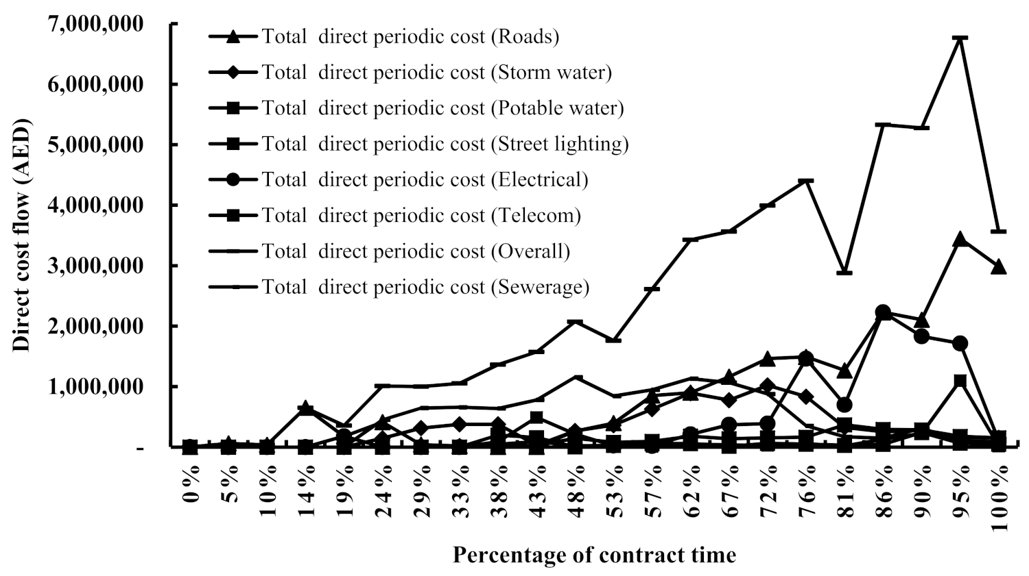
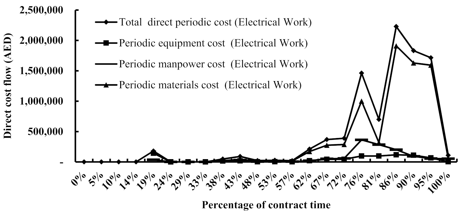
This subsection investigates the cost flow’s underlying patterns at the work package level; hence, the periodic total direct cost flow profile for each individual work package has been plotted in the graph shown in Figure 3. According to Figure 3, the deepest distortion, which was experienced at 81%, was caused by both the road and the electrical works. It has, therefore, been decided to further investigate the cost flow profiles for the individual cost components forming the total direct cost of these two packages to identify the cost component(s) responsible for this distortion and the associated reason(s) behind its occurrence.

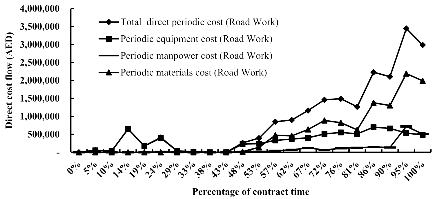
Accordingly, the periodic individual cost flow profiles for the road and electrical works have been plotted in Figure 4 and Figure 5, respectively, demonstrating that the deepest distortion observed at 81% was caused by a substantial reduction in the material cost flow profile, which had a considerable effect on the total direct cost profile of the project seen as a deep decay. This initially suggests that the production rate at the site was relatively lower in comparison with the preceding and successive interval points, thus resulting in a lower cost flow and, hence, a lower value flow, which indicates that there was either a shortage in the material supply or in the availability of the manpower to install the already supplied materials. However, the same figures demonstrate that the manpower cost flow was running at a steady pace at that point; in addition, the site records demonstrated that the materials had already been supplied to the site. Subsequently, when the site records were investigated to arrive at the root cause of this distortion, they revealed that during this period, the city in which the site was located encountered inclement weather conditions, including fog and heavy winds, that prevented the departure of the manpower from their labour accommodation; hence, the arrival at site was delayed. The late departure was due to statutory regulations prohibiting bus traffic movement on the roads to prevent accidents during heavy fog occurrences owing to low visibility. As a result, the production suffered substantial losses of productivity during this period since the actual working hours were less than that in the previous and subsequent intervals; however, the manpower received the same monthly wages, which caused the cost flow profile to continue to be constant.

The aforementioned root factor (i.e., inclement weather) was reported by [27] as the second highest ranked factor affecting the forecast of a cost flow; hence the forecast of the value flow and the net cash flow. The same factor was reported by [2] as one of the significant factors affecting the cash flow forecast in highway construction projects. In addition, [26] reported that production target slippage was the third highest ranked risk factor having an impact on the cost flow forecast. In contrast to [2,27], who identified the risks at an aggregate level, the present research has identified the cost component impacted by a given risk factor and the root risk that turned out to be dissimilar from the factor identified at the aggregate level. This must be emphasized in the domain of CFF because if a risk factor is identified at the preconstruction stage as influencing the cost flow of a project, its effect must not be quantified on the total cost flow forecast curve. Instead, the individual cost component that is likely to be influenced by the identified risk(s) must be identified and, subsequently, the effect of the risk is quantified on the forecast cost flow curve of that specific individual cost component.

Consequently, this study signifies the importance of identifying the impact of the root risk factors on the individual cost flow rather than on the aggregated cost flow of a given construction project. For instance, an external party away from the present case study project would forecast that the aforementioned distortion might have occurred due to material shortages or due to improper performance of the manpower. However, the root risk factors identified at the micro-level were inclement weather and slippage in the production rates caused by the former. Further analysis with respect to risk is outside the scope of this research.

4.2. An Illustrative Heuristic Graph Characterizing the Cost Flow of Infrastructure Projects

To visually illuminate the patterns of the cost flow trends discussed earlier, a graph has been plotted in Figure 6 that demonstrates the dominance of the individual cost component, as well as the work package during various time intervals of a given infrastructure project represented by the case study. The graph is divided into five distinct zones to characterize the dependency of the aggregated cost flow in accordance with the dominance of a given cost component, as well as a given work package.

In this context, during the primary zone (from 0% to 10%), the total cost flow is a function of the indirect cost flow, whereas during the secondary zone (10% to 19%) and tertiary zone (19% to 53%), the total cost flow is a function of the equipment allocated for the earthwork package and the sewer and, stormwater packages due to the reasons described previously. On the other hand, the quaternary zone (53% to 91%) is influenced by the material cost flow of the road work and the electrical packages. In this zone, the cost flow is highly vulnerable to a distortion that has a relatively high convex impact on the total cost flow, as the various work packages are executed simultaneously; thus, even if a relatively low-risk factor takes place, its impact will be high at the aggregate level and probably irrecoverable in the short term, unlike in the previous zones, where only limited work packages are executed due to the constrained dependency where the effects of an occurred risk are recoverable within a relatively short time. During the final quinary zone (91% to 100%), the material cost flow continues to dominate the picture with a decline towards the end, with the manpower cost flow exceeding the equipment cost flow.

The starting point of the quaternary zone is important, as during this zone, the cost flow is highly vulnerable to adverse factors, the effects of which are irrecoverable in the short term, thus resulting in a prolonged negative impact on the cost flow and, hence, the value flow and the net cash flow. Therefore, determining/identifying the commencement of this zone during a project duration proactively assists in reducing the effects of the occurrence of highly undesirable factors. This point in time can be termed as “the quaternary flow percentage” at which the cost flow starts to accelerate in a manner different from the previous periods, after which the vulnerability to risk is relatively high with high effects. Within the context of the current case study, the quaternary flow was found to take 53% of the contract duration. Furthermore, it is also significant to note that the cost flow’s geometric patterns repeated themselves, although at different scales (i.e., cost flow intensity). For instance, it took the direct cost flow 14% of the contract duration at the commencement of the project to reach the first peak. This is the same percentage taken to reach the fourth peak observed from 81% to 95%.

This proposed graph-based heuristic holistically visualizes the cost flow behavioural patterns of the built-in data of the CFF model that will be developed and presented in the subsequent section. However, the indications in Figure 6 are not necessarily applicable to all projects. As highlighted earlier, such an illustrative graph in the literature is absent, which might be one of the main reasons that limited the application of the existing CFF models in practice. Furthermore, this zoning graph is argued to provide a new dimension for project classification, as it offers a platform for comparison purposes of the cost flow and cash flow and it facilitates the exchange of data. In particular, the coined term “the quaternary flow percentage” can serve as the defining point distinguishing the cost flow behaviour of various projects.

4.3. The Development of the Cash Flow Forecasting Model

This section paves the way to modelling the net cash flow forecast based on the cost flow forecast that is developed by deriving the parameters (Alpha and Beta) for the logit-transformation function using the cost dataset of the case study project. This is done in order to derive the cumulative cost flow forecast percentage at each period of a given infrastructure project. As each individual cost component has exhibited a unique cost flow behaviour, it is irrational to forecast the cost flow and, hence, the net cash flow, based on the aggregated cost flow (i.e., the total sum of direct and indirect costs). Instead, the cost flow for each individual cost component needs to be forecast separately, thus leading to the forecast of the total cost flow and, subsequently, the net cash flow after determining the value flow.

4.3.1. Fitting Parameters (Alpha and Beta) Using the Logit Transformation Technique

To derive the fitting parameters (i.e., Alpha and Beta) to fit an S-curve function into the cumulative cost flows to forecast the cost flow of the individual cost components, a spreadsheet was designed using Microsoft Excel to derive the constants α (intercept) and β (slope) using the equations introduced earlier by following the detailed procedure outlined in [5] (p. 94). As a consequence of using the actual cost flow data of the case study project, the fitting parameters along with the accuracy of fit denoted by SDY for each cost component, as well as for the aggregated cost, have been derived to form the cumulative cost flow forecast curves, which are listed in

Table 4. The fitting parameters (Alpha and Beta) for the developed model.

Serial Number	Cost Component	The Case Study Project Data			Parameters Reported by [27]			Parameters Reported by [5]
		α	β	SDY	α	β	SDY	α	β	SDY
1	Materials	−2.3184	1.6642	2.41	Not available	Not available	Not available	Not available	Not available	Not available
2	Manpower	−2.0457	1.7559	5.29
3	Machinery	−0.7290	1.4703	2.34
5	Total direct	−1.6707	1.5523	2.72
4	Indirect	0.2199	1.0026	3.54
6	Total cost (direct + indirect)	−1.0982	1.1720	1.05	−1.3620	1.5869	1.91	−0.8200	1.1300	2.18

below.

Comparing the derived values of the parameters at the aggregate level with the averaged ranges reported by [5,27] has revealed that the values are within the reported ranges. Furthermore, the values demonstrate a good fit; hence, the results were encouraging due to relatively low values of SDY [5] (p. 49). On the other hand, the Alpha and Beta values derived for each individual cost component could not be compared with others, as the relevant literature lacks such values at the resource level; therefore, the respective cells in Table 3 have been marked as not available. In the same vein of comparison, the Alpha and Beta values at the aggregate level of the dataset of the case study project practically resemble the corresponding values reported in [20] derived for building projects procured through the management contracts route, which ranged from −0.948 to −1.372 and 1.696 to 1.328 for Alpha and Beta, respectively. This observation mathematically underpins the previous findings elaborated earlier, thus demonstrating that the studied infrastructure project procured through the traditional route has behaved, in terms of the cost flow, in a similar manner to building projects procured through the management contracts route as a result of the reasons mentioned earlier. 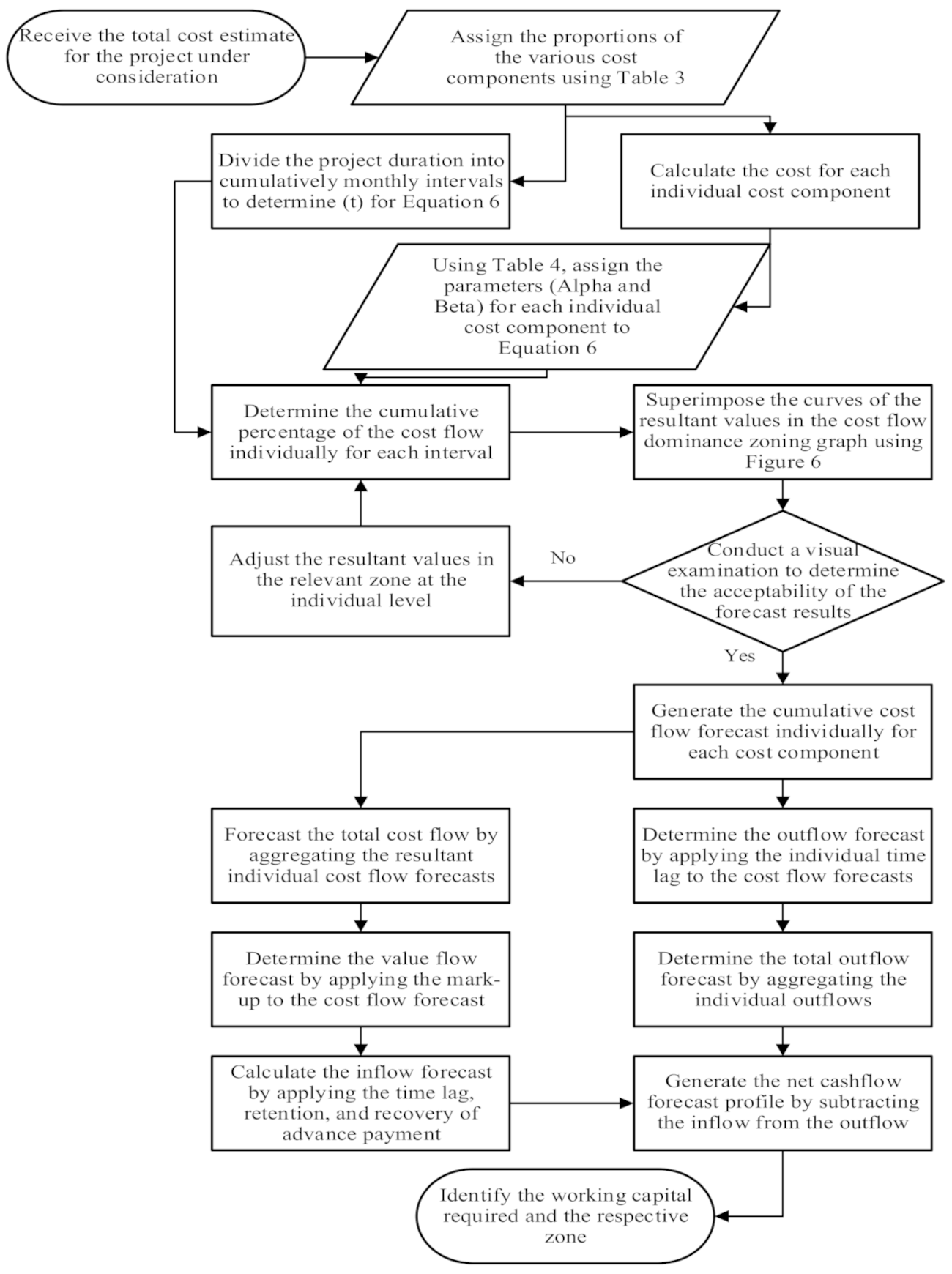In terms of the individual cost flow behaviour, Table 4 indicates that the inconsistency in the values of Alpha and Beta for each cost component underpins, based on mathematical evidence, the previous findings reported earlier stating that the cost flow behaviour for each cost component follows a different pattern than the others. To assist in implementing the proposed model in practice, a flowchart has been designed, as demonstrated in Figure 7.

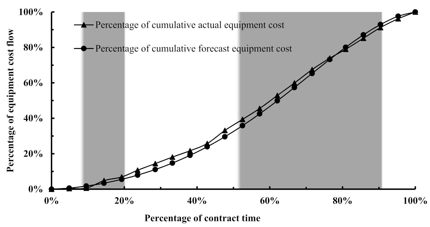
4.3.2. The Cost Flow Forecast

Following the steps of the flowchart illustrated in Figure 7, the cumulative cost flow forecast curves of the case study have been derived so as to perform an initial test for the model. The resultant forecast curves (i.e., the fitted curves) along with the actual curves are visualized in Figure 8, Figure 9, Figure 10, Figure 11 and Figure 12 on the dominance zoning graph presented in Section 4.2 to draw a comparison between the actual and forecast cost flows on a common platform and to determine the zone at which the under/over forecast has taken place.

The preceding figures relating to the direct cost components illustrate that the cost flows have been under-forecasted in the tertiary zone and have continued this trend in the quaternary zone up to 81% of the contract duration, where a shift in the forecast trend has taken place, turning into an over-forecast. It is worth noting that the under-forecast trend would have continued towards the end of the contract, but due to the deepest distortion embedded in the dataset based on which the fitting parameters were derived; thus, the forecast trend has shifted. This indicates that the logit function has provided a smoothness in the forecast trends.

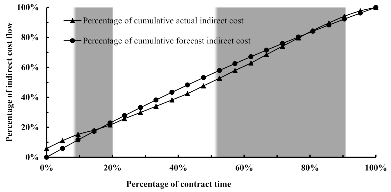
As far as the dominance of a given cost component is concerned during a particular zone observed based on the behaviour of the actual cost flows, Figure 8, Figure 9, Figure 10, Figure 11 and Figure 12 reveal that the cost flow of a given cost component tends to be under-forecasted during its dominance period. This is pronounced for the equipment and materials cost flows that dominated the total cost flow picture during the tertiary and quaternary zones, whereas the cost flow forecast of the indirect cost has been under-forecast during the primary zone, which was dominated by it.

A visual inspection of Figure 12 reveals that the overall cost flow forecast tends to be slightly higher than the actual cost flow. This reverse in the under/over forecast in the cost flow observed at the aggregate level, which differs from what is demonstrated at the individual level, has been attributed to the significant contribution of the indirect cost flow forecast to the overall cost flow forecast. The significant effect of indirect cost component on the aggregated cost flow forecast demonstrates the importance of incorporating its forecast in the overall cost flow forecast to balance the under/over-forecast generated individually, as the indirect cost behaves in a parabolic manner, whereas the direct cost takes the shape of a polynomial function according to the cost flow behaviour investigated earlier.

Accordingly, the logit transformation equation tends to generate an over-forecast for the cost flow that behaves parabolically in real life. However, it generates an under-forecast for the cost flow that actually behaves in a polynomial manner.

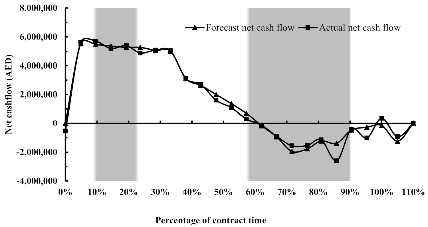
4.3.3. The Net Cash Flow Forecast

To arrive at the net cash flow forecast profile, the components of the following relationship are required to be determined:

Net cash flow = Cash inflow − Cash outflow

(8)

In this regard, the inflow forecast is a reflection of the value flow forecast, which is, in turn, generated from adding the mark-up rate to the total cost flow forecast in addition to the application of the contractual time lag of 30 days on the value flow forecast. Moreover, the advance payment along with its recovery at the contractual amortization rate, as well as the retention, have been taken into consideration. In addition, the common practice of the client’s advance payment for materials on site was invalidated. It shall be noted that due to commercial confidentiality purposes, the mark-up rate has not been applied; instead, the project has been assumed to be breakeven. In the same vein of Equation (8), having generated the cumulative percentages of the cost flows, the next step is to forecast the outflow curve for the project by aggregating the individual outflow curves, which are derived by multiplying the estimated cost for each cost component by the respective forecast percentage and applying the respective time lags separately for each individual cost component. This separation is required, as it would be irrational to assume a linear distribution of the individual costs throughout a given contract. Therefore, a CFF model that is built on aggregated cost flow data will likely be inaccurate.

In terms of the estimated costs, the actual cost for each cost component at the completion of the project has been considered for the testing purposes, as shown in Table 3. Subsequently, aggregating the individual forecast outflow curves has generated the total outflow forecast curve of the project. On the other hand, the actual time lag for the materials is two months, whereas the time lags for the other cost components, including the indirect cost, is zero (i.e., the costs are paid at the end of each month during which the cost has been incurred). Having determined the terms of Equation (8) has resulted in generating the net cash flow forecast profile visualized in Figure 13 below. The actual net cash flow profile of the case study has been superimposed for comparison purposes.

A visual examination of Figure 13 reveals that the net cash flow profile resulting from the developed cost flow forecast model has demonstrated a promising ability to forecast the net cash flow, as the trend of the forecast profile has conformed to the actual profile, in general. However, variances are observed at the end of the tertiary zone and during the quaternary zone, whereas during the primary zone, the model was unable to forecast the cash-out paid to the insurance, which is denoted by a negative value. This is attributed to the smoothing generated by the logit transformation technique on the actual cost flow trends when the fitting parameters were generated. Consequently, a forecast with relatively high accuracy for the required working capital denoted by a negative value can be derived.

4.4. Validation of the Proposed Heuristic CFF Model

To validate the accuracy and reliability of the proposed model, the cost flow and the subsequent net cash flow of case study (2) have been forecast using the procedure outlined in the flowchart visualized in Figure 7. For purposes of simplicity, the actual proportions of the individual cost components at completion demonstrated in Table 3 have been used to derive the cost outflow and the inflow by considering a zero mark-up rate which allows the net cash flow forecast to be derived. In implementing the proposed model by a prospective user, the proportions shown in Table 3 are believed to be highly representative of projects similar in nature to the case studies. Thus, it is recommended to use them if such values are not available. Subsequently, a comparison between the forecast and the actual cost flow has been performed based on the SDY values indicated in

Table 5. SDY between the forecast and actual cost flow curves.

Serial Number	Cost Component	SDY (Between the Forecast and Actual)
1	Materials	6.16
2	Manpower	7.17
3	Equipment	3.01
4	Total direct	3.29
5	Indirect	3.50
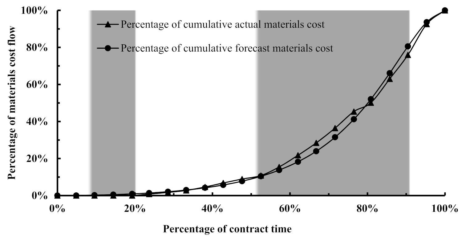
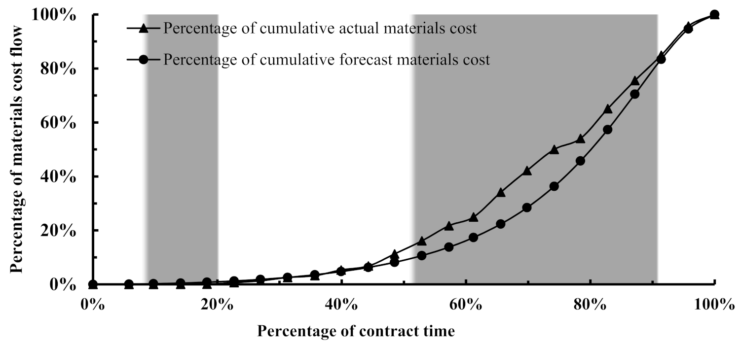
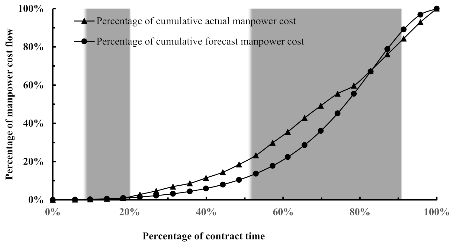
6	Total cost (direct + indirect)	2.59

below, whereas the net cash flow has been forecast and superimposed over the actual one in Figure 14 and 15 for the material and manpower cost flow, respectively

Table 5 indicates relatively high SDY values for the materials and manpower cost flows compared to the SDY values for the equipment and indirect cost flows; however, the SDY values have been found to be in line with the acceptable ranges reported in [5] (p. 55). To visually determine the zone at which the substantial variance has taken place that has contributed to the high SDY values, the forecast and the actual cost flows of those two components have been superimposed on the zoning graph, as demonstrated in Figure 14 and Figure 15.

Both Figure 14 and Figure 15 indicate that the model has under-forecast the cost flow for the materials and manpower in the quaternary zone, which caused the SDY values to be higher compared to the SDY of the other cost components. This demonstrates the susceptibility of the cost flow forecast accuracy to the material and the manpower costs for the work packages that take place after the quaternary flow percentage. Despite the under-forecast of these two cost components at the individual level, the model has been able to demonstrate its accuracy at the aggregate level of the project, as denoted by an SDY value of 2.59, which suggests that the model can reliably be used for another similar infrastructure project. It is interesting to note that as the SDY rises from the individual level to the aggregate level, it is reduced as a result of the consolidation and balancing of the errors of the various cost components. This reduction in the errors will be reflected in the net cash flow profile, which is the core objective of the model in which the financial decisionmakers are interested. Accordingly, the net cash flow profile has been achieved, as visualized in Figure 16.

The visual examination of Figure 16 suggests that the model has produced a net cash flow forecast profile in general agreement with the actual one. Although the model was unable to accurately forecast the working capital required during the quaternary zone at multiple intervals, the aggregated forecast in this zone substitutes for the actual individual working capital denoted at the negative side of Figure 16. This deviation between the forecast and actual results was expected during the quaternary zone, as the material cost flow was under-forecast previously.

5. Conclusions

This section highlights the implications and points out the perceived limitations. It further concludes the paper and paves the way towards future directions that could build upon the findings of this study.

5.1. Practical Implications

This study carries implications for practitioners in the construction management field because it has proposed a net cash flow forecasting model that can be used as a heuristic by contracting organizations involved in infrastructure development projects. The proposed heuristic model differs from the available models by offering detailed analysis of the underlying behaviour of the cost flow trends at both the resource and work package levels. Therefore, the model could reliably be applied in practice or its adopted methodology could simply be repeated by practitioners to derive new logit mathematical parameters. At an organisational level of contractors, the presented model might support contractors’ financial decision makers to forecast the required working capital and provide plausible evidence to banks when applying for short-term loans to finance a given project. As a result, this will enable them to arrange the working capital required ahead of time to avoid insolvency that adversely impacts the entire supply chain, whereas within the wider context it serves as a benchmarking tool. Using this, sustainable business growth and profitability in construction could noticeably be improved, as a result, financial and managerial continuous improvement in construction projects will materialise [38].

5.2. Theoretical Contribution

In terms of contribution at the academic level, this study responds to calls for identifying additional classification criteria for projects to enable more accurate CFF results [18,27]. Thus, it adds a new dimension to the existing dimensions reported in the literature (i.e., project duration, project type, procurement route, and project size) adopted in classifying projects in the field of cost and cash flow research. This new dimension is the characterization of the underlying behaviour of the cost flow profiles using the time- dependant zoning graph presented in Section 4.2 along with the introduced term “quaternary flow percentage”. This coined term could serve as a defining point distinguishing the cost flow behaviour of various infrastructure projects. As such, this study emphasizes the addition of this new dimension for the classification of projects based on the characterization of the behavioural patterns of the cost flow. Moreover, this study signifies the importance of identifying and assessing the impact of root risk factors on the individual cost flows and the individual work packages rather than on the aggregated cost flow of a given construction project. This is needed to derive an accurate cost flow forecast and, hence, a net cash flow forecast. Finally, the analysis methodology adopted paves the way forward to a new research branch that could revolve around forensic cost analysis, which could serve the construction claim industry with improved substantiation and quantification of disruption cost claims, for instance. This could be further investigated and verified in future research work.

5.3. Research Limitations

Despite the contributions as discussed, the findings of the study must only be applied with recognition of some limitations. Firstly, the study took place in the United Arab Emirates (UAE), and although it offered rich contextual insights into the phenomenon of cost flow behaviour in infrastructure projects and proposed a heuristic CFF model, it does not enable full generalisation to other types of projects. Having said this, this study provides a detailed cost flow analysis of a case study prior to employing its data sets to build the CFF model, the methodology of which could simply be replicated and applied in any other context. The second limitation revolves around the visual analysis of the cost flow profiles, which could be complemented by mathematical methods. However, from a practical perspective, visual analysis is regarded as a reliable method in the project controls field given its application simplicity to make fast informed decisions. A third limitation stems from the method applied to assess the forecasting accuracy of the model, which was by calculating SDY values only. The accuracy assessment of the CFF model could have been enhanced by adopting a quantitative approach using numerical error measures. However, despite the strengths offered by such an approach, it would have derailed the study from its defined methodological qualitative boundaries. Finally, the proposed CFF model does not demand the input of risk factors and uncertainty, which may materialise during a construction project. The reason behind this is that the impact of potential risk factors and uncertainty is implicitly embedded in the parameters (Alpha and Beta) derived from the logit technique. Another reason behind disregarding risk of delayed payments (cash inflow) from clients to contractors, for example, is the fact that infrastructure projects are generally financed by governments and international banks. Therefore, timely payments according to contract terms are highly secured.

5.4. Conclusion and Future Research

This study has critically reviewed and subsequently identified approaches employed to forecast the cost and cash flows for construction projects. Accordingly, the mathematical approach has been found to be effective to propose a parametric-based heuristic net cash flow forecasting model for infrastructure projects. In this regard, the logit transformation technique introduced in [5] was employed to derive the parameters (Alpha and Beta) for the proposed model. The proposed model has shown promising results, as the resultant cost flow forecast curves, which were the basis of forecasting net cash flow profiles, compared with the actual ones with high accuracy, as denoted by the relatively low SDY values. Comparing the derived parameters (Alpha and Beta) in this study with parameters reported in the literature has revealed that the cost flows of the infrastructure projects procured through the traditional route (i.e., D-B-B) behave in a similar manner to building projects procured through the management contracts route.

Furthermore, in contrast to previous research work [2,27] identifying the risks at an aggregate level of the cost/cash flow profiles, it has been concluded that the risk factors identified at the individual cost level tend to be dissimilar from the factors identified at the aggregate level. This has been determined following a detailed cost flow analysis performed initially at the aggregate level, at which the factors impacting the cost flow identified were the shortage of materials and improper performance of the manpower. However, the root factors identified at the individual cost level were actually the inclement weather and the slippage in the production rates caused by the former. Therefore, a future study that is worth conducting for infrastructure projects could revolve around modelling the impacts of weather conditions on the individual cost flow components of work activities. This could be achieved by collecting and compiling weather data from meteorological stations for various geographical areas during each day of the year and mapping the data to production rates of work activities outlined in daily reports from contracting organizations.