Article

A Life Cycle Assessment Approach for Vegetables in Large-, Mid-, and Small-Scale Food Systems in the Midwest US

1
Natural Resource Ecology and Management, Iowa State University, Ames, IA 50011, USA
2
Agricultural and Biosystems Engineering, Iowa State University, Ames, IA 50011, USA
3
Horticulture, Iowa State University, Ames, IA 50011, USA
*
Author to whom correspondence should be addressed.
Sustainability 2021, 13(20), 11368; https://0-doi-org.brum.beds.ac.uk/10.3390/su132011368
Submission received: 15 August 2021 / Revised: 7 October 2021 / Accepted: 11 October 2021 / Published: 14 October 2021

Abstract

:
Although vegetables are important for healthy diets, there are concerns about the sustainability of food systems that provide them. For example, half of fresh-market vegetables sold in the United States (US) are produced in California, leading to negative impacts associated with transportation. In Iowa, the focus of this study, 90% of food is imported from outside the state. Previous life cycle assessment (LCA) studies indicate that food consumption patterns affect global warming potential (GWP), with animal products having more negative impacts than vegetables. However, studies focused on how GWP, energy, and water use vary between food systems and vegetable types are less common. The purpose of this study was to examine these environmental impacts to inform decisions to buy locally or grow vegetables in the Midwest. We used a life cycle approach to examine three food systems (large-, mid-, and small-scale) and 18 vegetables commonly grown in/near Des Moines, Iowa. We found differences in GWP, energy, and water use (p ≤ 0.001 for each) for the three food systems with the large-scale scenario producing more emissions. There were also differences among vegetables, with the highest GWP for romaine lettuce (1.92 CO2eq/kg vegetable) approximately three times that of leaf lettuce (0.65 CO2eq/kg vegetable) at the large scale. Hotspots and tradeoffs between GWP, energy, and water use were also identified and could inform vegetable production/consumption based on carbon and water use footprints for the US Midwest.

1. Introduction

Mitigating the effects of climate change is a key challenge of our time (per the UN Sustainable Development Goal 13 [1]). Climate change currently threatens both human and natural systems [2]. Although the US Department of Defense and the Intergovernmental Panel on Climate Change (IPCC) rank climate change as one of the most serious threats to life on the planet, only about 50% of Americans view climate change as a personal risk [3]. Activists of all ages in the US and around the world have taken to the streets to raise awareness and support policies that will reduce carbon emissions [4,5]. To hit the target of less than a total increase of 1.5 °C as set by the IPCC, carbon emissions need to be reduced by 45% over the next ten years [6]. Food systems are a major source of greenhouse gases, and they contribute between 19% and 29% of total anthropogenic greenhouse gas emissions (GHGE) world-wide [2]. Food systems include growing and harvesting plants and animals, processing, packaging, transporting, marketing, consuming, and disposing of food-related waste [7].
Dietary choices are an important contributing factor to food system GHGE, and they have been the focus of a number of studies—for example, Heller et al., in a literature review, found 48 studies examining the environmental impacts of different dietary patterns between 1998 and 2013 [8]. Life cycle assessment (LCA) studies in particular indicate that dietary choices can greatly affect GHGE at various scales [9,10,11,12,13,14]. Animal-based food products require significantly more carbon, energy, and water for production than fruits, vegetables, and grains [7,15,16,17,18,19,20,21,22]. Mohareb et al. [22] found that animal-based foods made up 77% of US food-related GHGE in 2010. An analysis of 14 studies conducted by Hallstrom et al. [23] found that broader adoption of vegan or vegetarian diets could reduce GHG production by up to 53% compared to reference scenarios. Weber and Matthews found that reducing meat consumption could reduce GHGE more than buying local food [24]. However, it is less clear how GHGE might vary between vegetable types and production scenarios, such as distant large-scale versus local medium- and/or small-scale food systems, and whether these alternatives could reduce carbon emissions at city or household scales.

1.1. Large-Scale (Conventional, Distant) Food Systems

Large-scale (conventional, often distant) food systems are important worldwide. In the US, large-scale farms produce the greatest proportion (42%) of food [25]. Important regional differences in GHGE associated with large-scale production are based on the local climate where foods are grown. For example, there is an almost seven-fold increase in energy used for pumping irrigation water for vegetable and fruit production in northern California compared to southern California [26].
Though important, food production processes themselves make up only about 25% of total food system energy use in high-income countries [27]. Transportation is another important component of the globalized food system. A conservative estimate is that typical grocery store produce items travel 2,400 km from farm to consumer [28,29,30,31,32]. Researchers who conducted another study found an average food transportation distance for the US of 6760 km [24]. In fact, in the US, 50% of fresh-market vegetables sold in 2016 were produced in California, despite water shortages there [33].
The potential negative impacts of increasingly globalized food trade have led to greater interest in local food production to reduce food miles and support for the idea that shorter food supply chains might mitigate this problem [32]. However, the importance of local food production in this regard may be overstated. Kreidenweis et al. found that only 4% of global warming potential (GWP) was associated with food delivery from producer to retailer, with greater impact at the food production stage [34]. It is also important to note that context matters: for northern cities such as those in the US Midwest, carbon emissions associated with heating greenhouses to grow produce during winter can be greater than carbon emissions associated with transportation of food from non-local production areas which grow outdoors year-round [35].
In 2018, it was estimated that 103 million tons of food was wasted in the US with residential waste making up about one quarter of the total [36]. Food waste is a key obstacle to reducing food system emissions. Landfills and wastewater treatment of food waste contributed about 12% of total US food system carbon emissions in 2010 [22]. Vegetables rank second among food groups for waste production, contributing about 19% of total food waste in the US and surpassed only by meat (including poultry and fish), which contributes to 30% of total food waste [37]. Enhancements of local food systems could help reduce food waste by using shorter supply chains, reducing both distance and time from farm to fork [32].

1.2. Mid-Scale (Commercial, Local) Food Systems

The mid-scale (commercial, local) food system includes urban and peri-urban agricultural production (UPA) of vegetables sold to local markets. According to the USDA, there is no standard definition for local; it can differ based on a variety of social and spatial factors [38]. However, in one US study, investigators found that consumers were willing to pay more for local when it was defined as production within 25 to 100 miles versus production at a distance of 400 miles [39]. UPA constitutes about 6% of all cropped land areas [40]. This land is found in a variety of settings. In one study of US UPA, researchers found that about 45% of UPA was in residential gardens, 21% in community gardens, and 27% on vacant lots [41]. There is enormous potential to strengthen UPA food production by increasing land availability for UPA. Local food systems could be further strengthened by localizing food manufacturing strategically based on the potential to improve environmental and social outcomes [42]. Growing food for local markets in the Midwest could reduce emissions by reducing transportation distances, food waste, water withdrawal, packaging, and emissions from cooling in transportation and retail [18].
A wide range of social, economic, political, and health benefits are also linked to UPA [43,44,45]. For example, a community economic impact assessment in northeast Iowa found that every USD 1.00 spent on local food helped to create USD 14.60 of investments in local food and farm operations [46]. Other social benefits of UPA can include increased food resilience, food security, and environmental justice for marginalized and low-resource populations [47,48]. Health benefits include reducing blood cholesterol levels and maintaining a healthy blood pressure [49,50].

1.3. Small-Scale (Home Garden) Food Systems

Household gardens are an important piece of the local food puzzle. In 2014, about 31% of US households engaged in their own garden food production [44]. Home gardens have many health, social, and financial benefits, such as increasing vegetable consumption (by two servings each day for gardeners compared to non-gardeners), reducing food costs, and maintaining family food culture [42,49,50]. Although motivations for producing food in home gardens vary widely, access to a home garden was found to be positively correlated with increases in both number of servings and diversity of fruit and vegetables consumed (based on data from a survey of over 500 residents in Iowa [51]). These survey results also indicated that a smaller number of urban residents had access to a home garden than did residents in rural areas.
Despite the significance of home garden production, the connection between home gardens and food security in the literature is unclear [52]. In one study conducted to examine home gardening and food insecurity in the Midwest, researchers were unable to conclude that there was a relationship between them, raising questions as to whether home gardening can have an impact on household food security [53]. In another set of studies, investigators found that food production in home gardens and nutritional status of children less than five years old were also not closely correlated, although the strength of the relationship varied by both city and personal circumstances of respondents [54,55].

1.4. Using a Life Cycle Assessment Approach for Food Systems Modeling

The ability to assess food systems is an important first step to enable the design of systems that produce less environmental impact. Life cycle assessment (LCA) can be used to measure emissions produced by food systems (among other things) from production to transportation and consumption, identifying environmental impacts at each stage [9]. LCAs can have varying system boundaries which can span from cradle to grave (raw resource extraction to product disposal) or more recently from cradle to cradle (raw resource recycled back to raw resource) [56,57]. Lack of uniformity between studies (in definition of functional units and system boundaries) is an important challenge to making valid comparisons among previous LCAs conducted for food system analysis [9,21]. In addition to standardizing system components, combining LCA with other assessment tools that integrate social and economic factors (e.g., LCA with technoeconomic assessment (LCA-TEA)) could provide results that more directly apply to policy development and decision-making [12].
Trade-offs between food production, water use, and energy requirements within UPA food systems can be identified using an LCA approach. In many cases, UPA may not reduce food system energy demands [26]. Selling directly to consumers without packaging can reduce energy use and GHGE associated with local foods, especially fresh fruits and vegetables for which packaging is a large portion of total energy use [58]. However, with limited resources, some local governments may find that UPA is not the most effective way to confront issues such as food insecurity, finding that focusing on employment policies could more quickly improve food access and community health [59]. Higher prices for locally grown produce could also deter buyers, especially those affected by food insecurity.
Many LCA studies have been conducted to examine the carbon footprint of individual foods at a variety of scales [18,21,35,60,61]. Selecting foods based on information on emissions uncovered through LCA is an important step for reducing the climate change impact of food systems [60]. In one study, investigators found that, if populations in the north ate more seasonal diets (e.g., more fruits and vegetables when they are in season) and consumed less meat, additional local food production could result in reduced environmental impacts [21]. Providing a comprehensive comparison of vegetables for current food systems could help producers and consumers alike make better informed decisions that have fewer negative environmental impacts.

1.5. Objectives

The purpose of this study was to understand the environmental impacts of vegetables within three different types of food systems to inform more sustainable decision-making based on carbon and water footprints. We analyzed the emissions of vegetables throughout their lifecycle, from cradle to grave (seed to disposal). Using the Des Moines Metropolitan Statistical Area (a six-county area surrounding Des Moines, IA: the DM MSA) as a case study that is representative of other urban areas in the rainfed upper Midwest, we used an LCA approach to examine carbon emissions, energy consumption, and water use for eighteen vegetables commonly grown and sold commercially in Iowa. We assessed the vegetables under three food system scenarios; a large-scale (conventional, distant: LS) food system was compared to two alternative food system scenarios, a mid-scale (commercial, local: MS) and a small-scale (home garden: SS) system. Next, we identified hotspots and tradeoffs for GWP, energy, and water use by food system component and vegetable type. Finally, we compared vegetable types to develop a comprehensive analysis of carbon and water footprints to inform producers, policy makers, and educators in a variety of contexts. The results could also be useful for commercial producers who sell locally and/or by home gardeners to design their own production systems based on carbon and water footprints. The information generated could also be used to assist consumers who wish to reduce their own environmental footprint through selection of certain foods or other forms of targeted local purchasing.

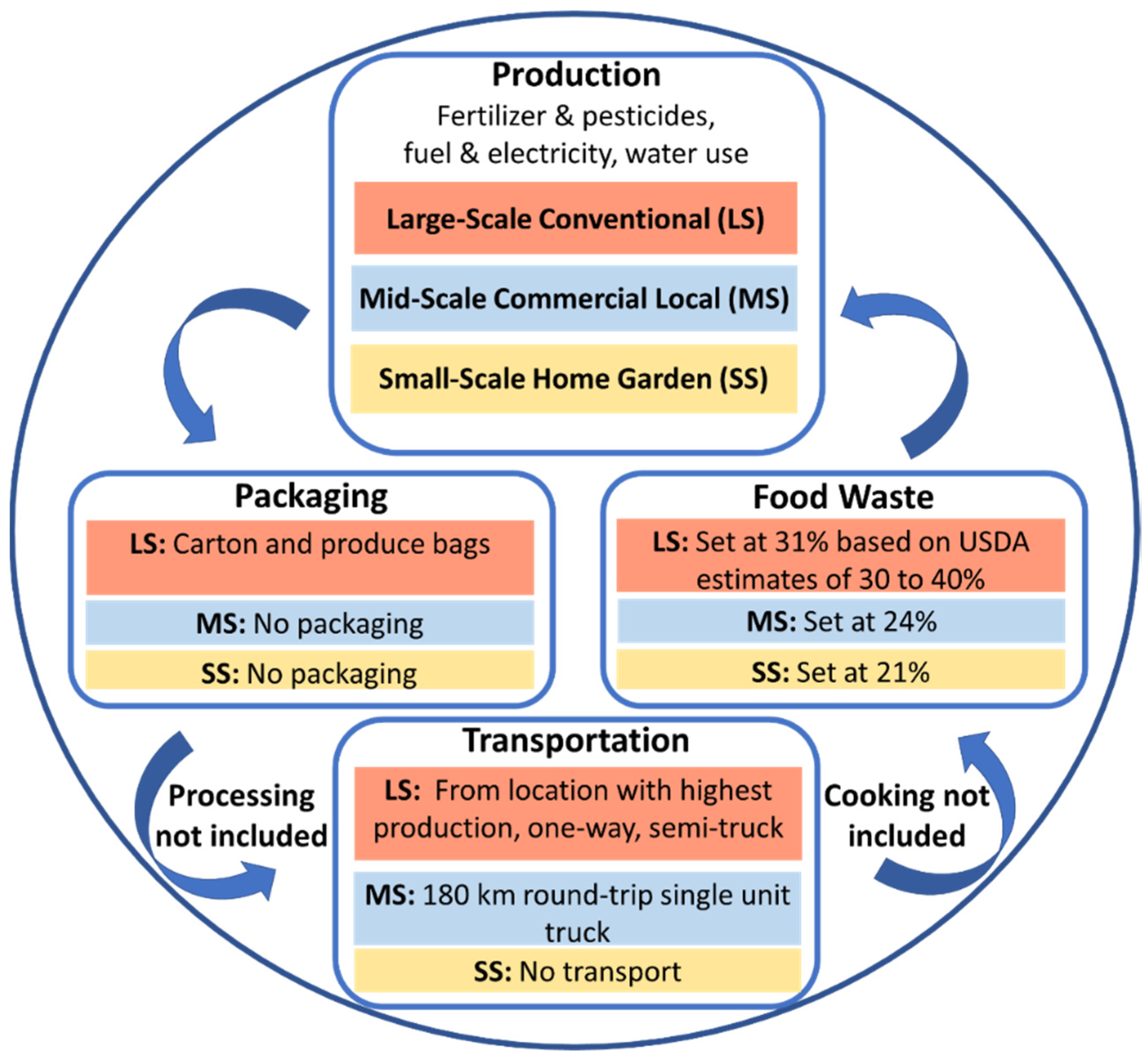
2. Materials and Methods

The focus of this research was to provide reasonable estimates for vegetable emissions throughout the food system for 18 vegetables and three scenarios using an LCA approach. Carbon, energy, and water footprints were developed using the modeling platform FoodCarbonScope™ (CleanMetrics, 2020). This software incorporates many proprietary US datasets and developed life cycle impact assessment (LCIA) methods that comply with current international standards (e.g., ISO 14040 [62]). FoodCarbonScope™ also uses data from the IPCC Guidelines for National GHG Inventories to inform baseline models through research-based methods for estimating anthropogenic GHG emissions [63]. The system boundary was cradle to grave, including production, packaging, transportation, and food waste (Figure 1). Processing and cooking were not included in this LCA because all vegetables we assessed are typically sold fresh, and variation in cooking methods would make comparisons between vegetable types and scenarios more difficult. All comparisons were made based on emissions created or resources used per 1 kg of food consumed as the functional unit and incorporated a level of food waste that was constant within each scenario.
Vegetables were chosen as the target food group for this study for three reasons. First, vegetables make up 22% of US food consumption and contribute to nutritional security by providing important micronutrients. Vegetables support a host of important health benefits, such as reducing blood cholesterol levels and maintaining a healthy blood pressure [47,48]. Second, vegetable production systems are easy to integrate into urban environments where about 80% of the US population currently resides [64]. Third, the shorter shelf-life of most vegetables make them more likely to be wasted in long supply chains than other food crops and therefore important to study from an environmental impact perspective.
Specific vegetables selected for this study were those that met three criteria: (1) they are currently grown by farmers in Iowa according to their relative production areas in the 2017 United State Department of Agriculture (USDA) Census of Agriculture by State [65]; (2) there are relevant US field models included in the FoodCarbonScope™ LCA modeling software; and (3) US consumption data indicate their importance according to the USDA 2016 loss-adjusted food availability (per capita) data system [66]. Eighteen vegetables which met all three criteria were analyzed based on the three production scenarios (Table 1).

2.1. Large-Scale (LS) Scenario

In the large-scale (conventional, distant; hereafter referred to as LS) scenario, we assumed vegetables were produced in the state and the county with highest production for each of the 18 vegetables sold fresh in the US. Most vegetables were produced in California (14), with additional vegetables grown in Florida (2), Minnesota (1), and Idaho (1), all US. Production practices and yields were integrated into the model based on a combination of available literature and extension publication. Assumptions in the LCA models in FoodCarbonScope™ that did not match these production scenario locations available in the model were adjusted for water use and electricity (for pumping water) using state-specific USDA agricultural census data [67,68] and are explained in the Supplemental Materials (Spreadsheet S1: Additional Model Assumptions). Four out of 18 vegetables modeled required state-specific adjustments. Pesticide and fuel use were adjusted for three vegetables for which state-level data were not available using proxies from the scenario-specific state and scale. Snap beans were assessed as green beans of the “Blue Lake” variety grown conventionally in California (CA) USA, and cucumber and pumpkin were assessed as “summer squash” grown conventionally, also in CA.
Packaging weights in the LS scenario were determined using extension resources and online catalog lists of typical shipping container materials and sizes [69,70]. To make comparisons between vegetables, we assumed all vegetables were shipped in bulk without additional in-store consumer packaging aside from a produce bag commonly used in fresh produce sections in grocery stores in the Midwest US. Wooden pallets common for transportation by semi-truck trailer were not included because they are often reused and/or recycled, and this packaging material was not available in the modeling software. We also assumed that all packaging material waste would be transported 90 km by single-unit truck and disposed of in an uncategorized landfill.
Typical transportation distances for the LS scenario were selected based on the state with the highest production for each vegetable. Again, for most vegetables in this study, this was California. The county with the highest production of this vegetable within the state was set as the starting point to measure distance using Google Maps. We chose central Des Moines as the common end point (at the intersection of 6th Avenue and Locust Street) for all vegetables [71]. We assumed all vegetables were cooled in transport and stored without cooling in retail settings.
In the LS food system scenario, waste was set as constant for all vegetables at the national average of 31% [37]. This source may overestimate food waste by combining household and food service waste streams and by using a mass balance method instead of direct measurements of food waste [72]. We used this source because we were able to choose both the food waste type (fresh vegetables) and the food system stage (retail versus consumer), a level of specificity which was not available in more recent studies. We assumed all food waste and packaging materials were transported 90 km by a single-unit truck to an uncategorized landfill.

2.2. Mid-Scale (MS) Scenario

The mid-scale (commercial, local; hereafter referred to as MS) scenario was adjusted from the large-scale conventional scenario (Table 1) with a full explanation of the adjusted assumptions available in Supplemental Materials (Spreadsheet S1: Additional Model Assumptions). Given the scale of individual vegetable operations in Iowa, 75% to 80% of growers sell their produce direct-to-consumer, usually through either community supported agriculture (CSA) or farmer’s markets without use of packaging [73]. For the MS scenario, we assumed all food was produced within the DM MSA, and 180 km in a single- unit truck was included to account for round-trip transport from the edge of the MSA spatial boundary to the urban center.
Pesticide use in the MS scenario is lower for Iowa growers than for those in other areas in the upper Midwest due to their smaller operations. Horticultural crop farms in Iowa are, on average, 3.20 ha, with a median size of 0.81 ha [74]. Among pesticides, fungicides are used sparsely, although insecticides and herbicides are more widely used [74]. We estimated pesticide use for each vegetable type based on the amount used in a “typical year” in Iowa by category (herbicide, fungicide, insecticide). The amount prescribed and the units of active ingredients (a.i.) vary based on the formulation of specific pesticides, as does the energy used to produce 1 kg a.i. between and within pesticide categories. The assumptions for this study were developed by author AN based on pesticides commonly used in the state of Iowa. We developed an estimate for the “typical” amount of energy used to produce 1 kg a.i. pesticide/ha/year for each vegetable type based on average pesticide production energy of 370 MJ/kg a.i., which is close to previous estimates of 361 MJ/kg a.i. [75]. To make conversions, each kg a.i. pesticide was assumed to produce 25.50 kg CO2 [75], and a factor of 0.069 kg CO2eq/MJ a.i. pesticide energy was applied to account for the standard 100 year GWP [27]. An average pesticide density of 1.078 kg/L was also applied.
Assumptions for fuel use for the MS scenario were estimated based on Iowa State Horticultural Research Station records and field trials with Iowa producers. Use of tractors/fuel consumption can vary based on operation characteristics (e.g., mechanical tilling, spraying, laying plastic mulch as weed control), condition of the soil, and equipment size (e.g., two- vs. six-row sprayer/harvester). We used fuel assumptions based on differences that arise due to farm operations but did not include variation due to soil condition and equipment size. Fuel use was assessed based on a 2.74 m (9.00 ft) tiller mounted on a 50-horsepower tractor, averaging 1.63 L diesel fuel/h.
Average Midwest yields were used when available; otherwise, USDA average yields for the US were used by vegetable type [76,77]. Manual harvest was assumed for all crops except snap beans, sweet corn, potato, peas, and carrot based on typical Iowa vegetable production practices. Onions and leafy greens were assumed to be direct seeded, not on black plastic mulch. For carrots and potatoes, mechanical digging was assumed to be followed by manual harvest. The same assumptions were used in both the MS and the SS scenarios for water use and electricity for irrigation. Water use and irrigation were both estimated based on USDA irrigation and energy expense information for horticulture operations by state [67,78].
For food waste, 21% of consumer-level waste and an additional 3% for distribution-level waste were added to account for potential loss in distribution (for a total of 24%) [37]. We assumed all waste was transported 90 km by single-unit truck to an uncategorized landfill. The MS scenario was also adjusted to account for regional and scale-based differences in the use of pesticides, fuel, water, and electricity (for water pumping) for vegetable production in the DM MSA (Spreadsheet S1: Additional Model Assumptions).

2.3. Small-Scale (SS) Scenario

The small scale (home garden; hereafter SS) scenario assumed that production included rototilling for one hour/season/garden with all planting and harvesting activities done by hand. The SS scenario used the same yield assumptions as the MS scenario and did not include packaging or transportation. Scale adjustments were made for pesticide and fuel use based on the average home garden size for Des Moines (168 m2 for each garden [79]).
Pesticide use for the SS scenario was based on typical use in US home gardens at the national scale using EPA home and garden pesticide use data and National Gardening Association estimates for home garden area in the US [80,81]. We made the same key assumptions for CO2 conversion and MJ/kg a.i. pesticide as for the MS scenario (Section 2.2, above). Assumptions for fuel use in the SS scenario include one hour using a walk-behind rototiller/garden/year at 0.47 L fuel/hour and an average yield of 167 kg/m2 based on the authors’ own gardening experience. We used the same state-level USDA irrigation and irrigation energy use assumptions for the SS scenario that were used for the MS scenario. For waste, we maintained the same 21% of food waste at the consumer level [37]. All waste was assumed to be transported 90 km by single-unit truck to an uncategorized landfill.

2.4. Linear Model

Linear models were developed in R to assess variance in scenarios using the “lm” function [82]. Each environmental impact (GWP, energy, and water use) was fit to the model for each scale without incorporating differences due to vegetable type. Model fit was assessed based on a t-test; p-values were reported to display the statistical differences based on scenario.

2.5. Hotspots and Tradeoffs

Hotspots refer to relatively high environmental impacts. Hotspots were identified by food system component and vegetable type and were compared for the three food system scenarios. For GWP, hotspots for production inputs including water pumping, pesticides, fertilizers, other farm inputs, electricity, and fuel (for tillage and pesticide application) were identified. CO2 and N2O are emitted due to soil tillage and were accounted for separately, and inputs beyond the farm gate such as fuel for transportation, packaging, and waste were also considered separately. Hotspots for each of the environmental impacts were examined using a “heat map” developed in R, with values increasing from dark blue (low impact) to bright yellow (high impact) [82]. Separate heat maps were created for each environmental impact to enable easy comparison by vegetable types.
Tradeoffs were assessed to identify environmental impacts by category (GWP, energy, and water). For example, a single vegetable can require high water quantity but low energy use (or vice versa). First, the correlation between the three impact categories were identified using a Pearson linear correlation by scale on a per-kg vegetable basis. High correlation indicates that the environmental impacts are not likely to produce tradeoffs, whereas low levels of correlation could produce tradeoffs. Next, vegetables were grouped using the Dietary Guidelines for Americans [83] to examine environmental impacts by group and to explore potential tradeoffs by impact category using a smooth histogram.

2.6. Environmental Impact Scores

An impact score was developed to capture carbon and water footprints for each vegetable by weight. This enabled a simplified incorporation of tradeoffs for each food system scenario assessed. The score was established based on fractional ranking; a mean rank was used for each equal rank value. This rank sum was then divided by two to give the impact score for each vegetable by scale. Equal weights were assigned to GWP and water use. The values were then categorized as low impact, moderate, and high impact.

3. Results

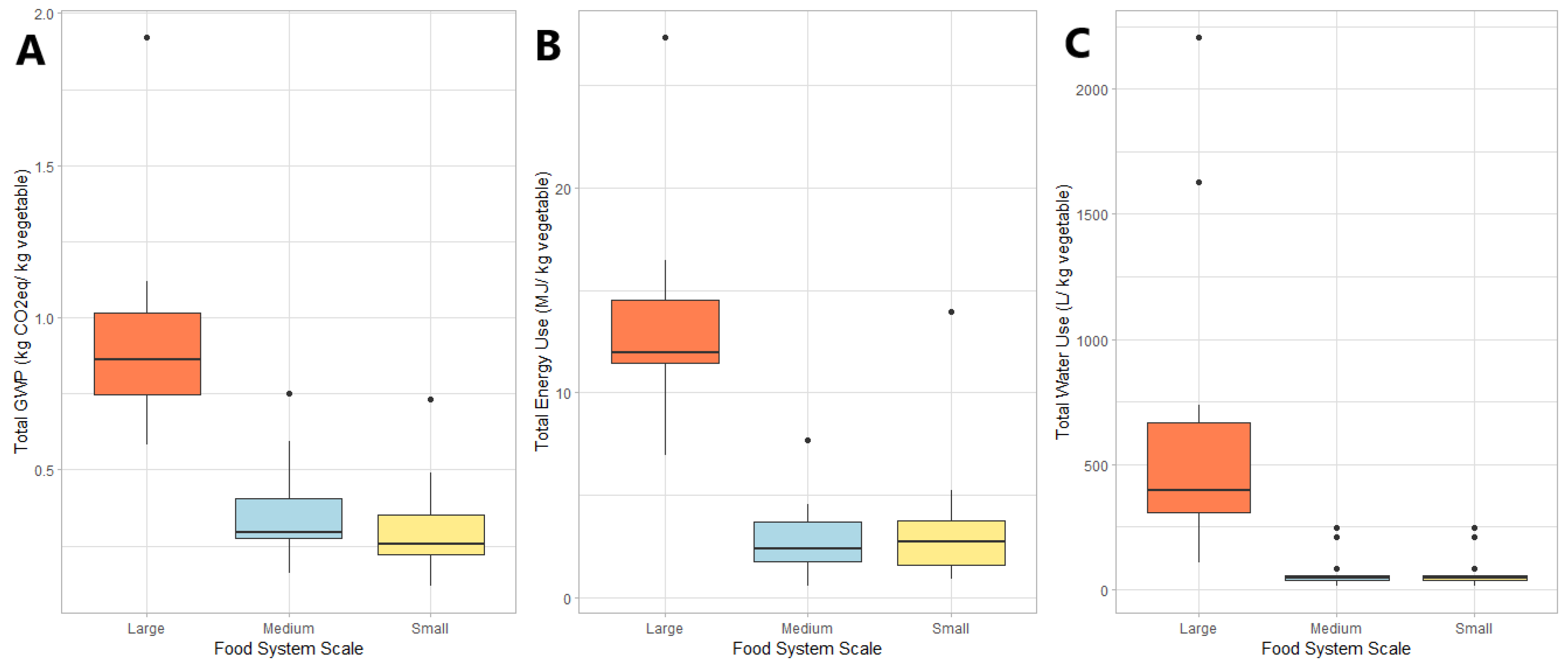
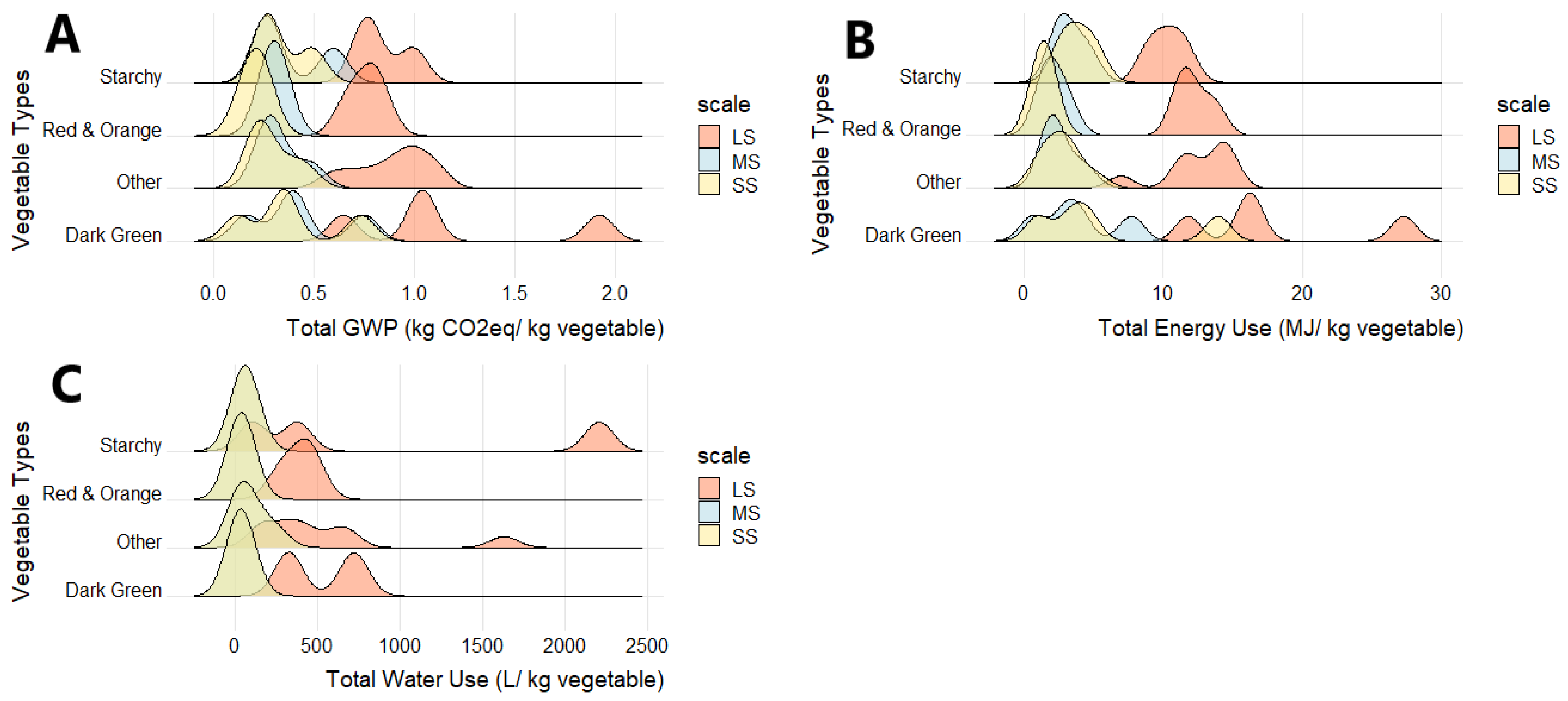
3.1. Global Warming Potential, Energy, and Water Use by Scale

Total GWP, energy, and water use/kg vegetable differed by scale based on linear models: GWP (p = 1.87 × 10⁻¹²), energy (p = 1.91 × 10⁻¹²), and water use (p = 3.98 × 10⁻⁶). The LS scenario produced greater total GWP/kg vegetable (coefficient estimate 0.92, p = 2 × 10⁻¹⁶) compared to the MS scenario (coefficient estimate −0.57, p = 9.28 × 10⁻¹¹) and the SS scenarios (coefficient estimate −0.61, p = 8.06 × 10⁻¹²). The MS and the SS scenarios had many overlapping values which varied considerably by vegetable type (Figure 2). The largest differences between scenarios were for water use. Both MS and SS scenarios used the same irrigation assumptions, and their water use average was 65.12 L/kg vegetable, whereas the LS irrigation assumptions were embedded in the LCA modeling software based on field studies, and the water use was 573.64 L/kg vegetable on average.

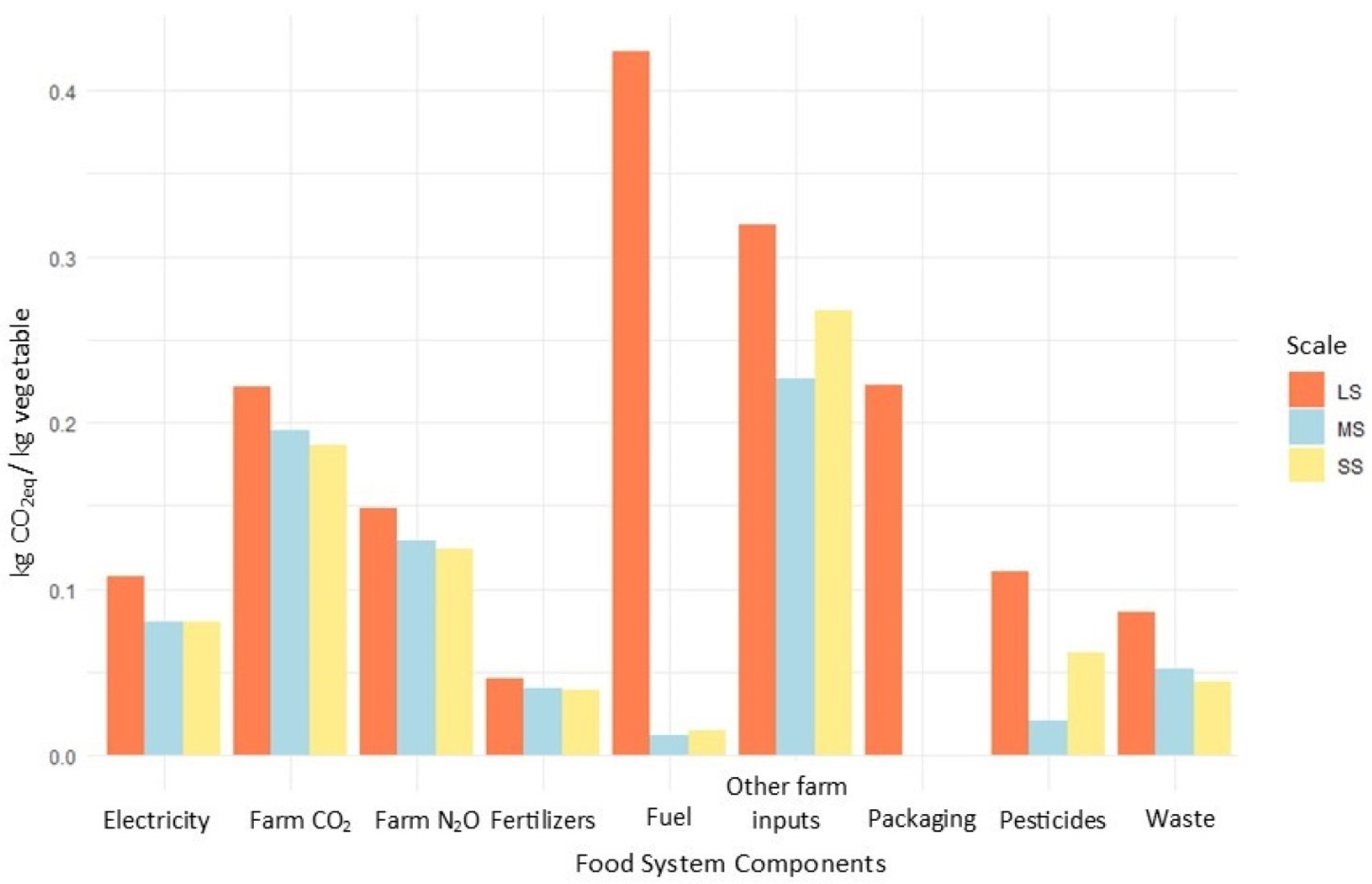
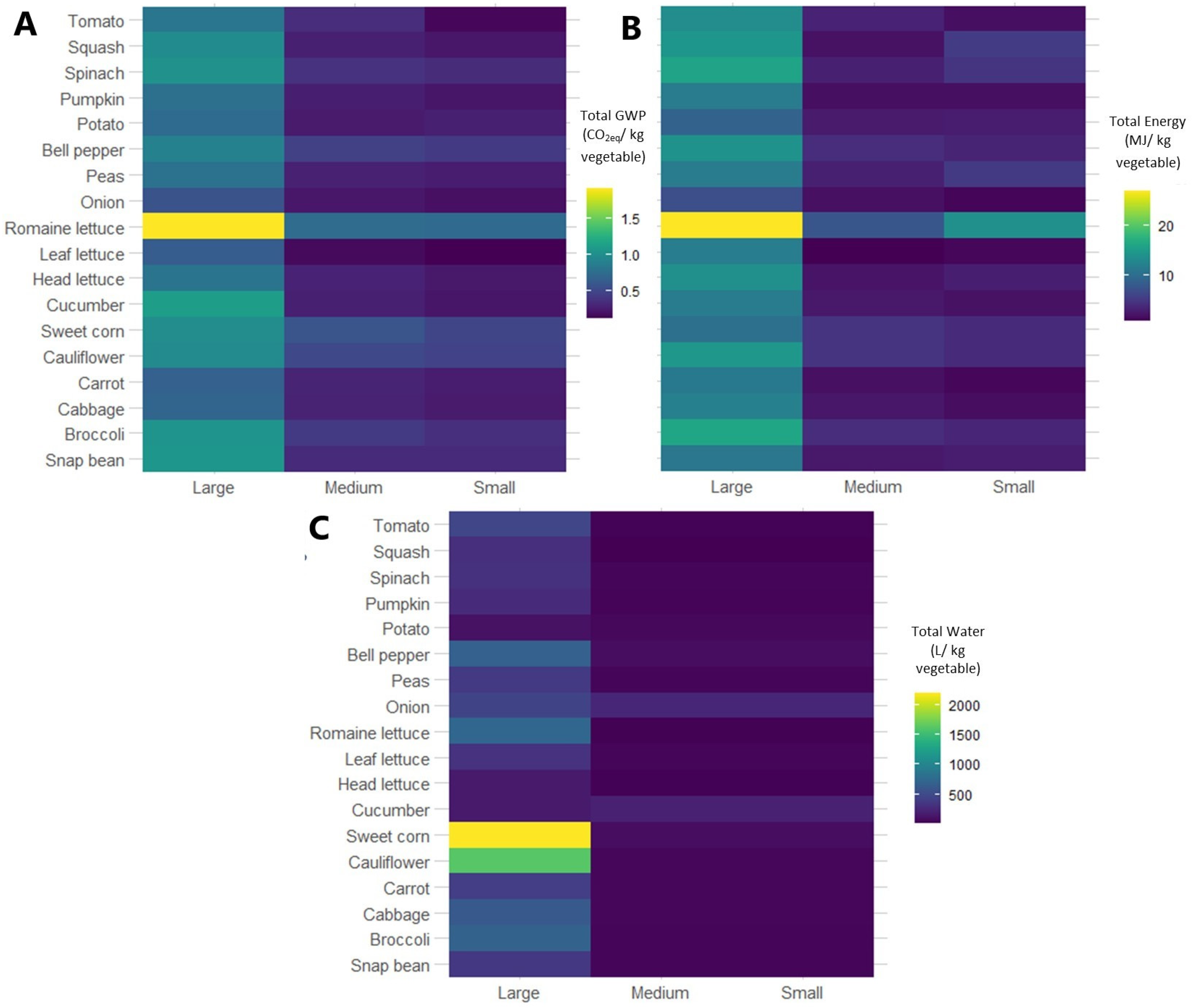
3.2. Hotspots and Tradeoffs for GWP, Energy, and Water Use by Scale and Vegetable Type

The LS scenario was associated with higher GWP than the MS and the SS scenarios for all food system components. There were several notable hotspots where the differences in average emissions for the three scales were high (Figure 3). Fuel use was a hotspot for which the CO2eq released in the LS scenario was about 15 times higher than that of either the MS or the SS scenarios. Packaging was another hotspot because it was a relatively large contributor to GWP in the LS scenario, but neither the MS nor the SS scenario included packaging.
There was variation in GWP, energy, and water used to produce 1 kg of the different vegetable types. Because of strong correlation between GWP and energy use, we did not detect tradeoffs or the hotspots for these similar variables (Figure 4). Romaine lettuce had a larger footprint for GWP and energy compared to all other vegetable types for all scenarios on a per-kg basis. The most marked difference was for the LS scenario where 1 kg of romaine lettuce was associated with 1.92 CO2eq and used 29.27 MJ energy. By contrast, for the LS scenario, 1 kg of leaf lettuce was estimated to be 0.65 CO2eq and 11.79 MJ of energy use, between a 2.5 and 3-fold decrease. Water use, however, was characterized by different hotspots that were only present in the LS scenario. Sweet corn and cauliflower used 2205 and 1629 L of water/kg vegetable, respectively, well above the average for the LS scenario (570 L/kg vegetable).
To better understand tradeoffs for GWP, energy, and water use for different food system scenarios for vegetables, linear correlations were developed for each output type and scale (Figure 5). There was correlation between GWP and energy use (r2 = 0.95) but less so for GWP and energy use with water use (r2 = 0.57 and 0.54, respectively).
In addition to differences for the three production scales, there were large ranges of GWP, energy, and water outputs on a per-kg basis by vegetable type. Vegetable categories from the 2015–2020 Dietary Guidelines for Americans (starchy, red and orange, other, dark green) were used to assess if differences in environmental outputs varied by vegetable groups which are nutritionally similar [83]. The difference within each vegetable category was greater than variation between vegetable categories for all outputs and scenarios, thus vegetable category was an ineffective way to assess environmental output (Figure 6).

3.3. Environmental Impact Score by Vegetable Type

Environmental impact scores were developed by combining carbon and water footprints into a comprehensive score. Impact scores were greatest for all vegetable types in the LS scenario. Between the MS and the SS scenarios, there were many overlapping values. Vegetables were categorized from lowest to highest impact score in three categories (Table 2). Leaf lettuce, head lettuce, onion, and carrot were all in the low environmental impact category in all scenarios. Additional vegetables in this category included potato in the LS and the MS scenarios and cabbage for both the MS and the SS scenarios. Aside from the lettuces, these are all less perishable vegetables, with the exception of tomato in the SS scenario. Cucumber and squash were within the moderate impact category for all scenarios. The LS and the MS scenarios both included tomato, while the MS and the SS scenarios had sweet corn, pumpkin, and bell pepper in the moderate impact category. The LS and the SS scenarios had no additional vegetables in common. The high impact category included romaine, broccoli, cauliflower, and snap bean for all scenarios. Romaine in the LS scenario had the highest impact score overall, though snap bean had the highest impacts within the MS and the SS scenarios. Vegetables in this category were generally more perishable than those in the low environmental impact category. The majority of vegetables in the MS and the SS scenarios fell into the same impact categories, though the specific rankings within each category did vary. The LS scenario showed larger variation in rankings compared to MS and SS.

4. Discussion

We assessed GWP outputs and energy and water inputs for three food system scenarios and 18 vegetable types commonly grown in Iowa to guide more environmentally conscious vegetable production and consumption. We found differences in environmental outputs by scale and identified hotspots and tradeoffs for them. Finally, the environmental impact score we developed in this study highlights some of the strengths and the weaknesses of the LCA approach and our carbon and water footprint framework.

4.1. Environmental Outputs by Scale

In this study, we found that the LS scenario had higher GWP and greater energy and water use than the MS and the SS scenarios on a per-kg vegetable basis for 18 vegetable types commonly grown in the Midwest US. Although we were unable to find similar LCA studies for vegetables produced in this region of the US, our results are similar to a fruit and vegetable LCA conducted in Sutton, South London, UK [18]. For that study, researchers compared output from an urban community garden to conventional commodity crop production. These researchers found that, for 16 fruit and vegetable types considered from production to point of retail, the community garden produced lower GHGE than the conventional food system with one exception (polytunnel strawberries) [18].
In another food system LCA conducted for the Lisbon, Portugal region, investigators found that local UPA food systems (including production to retail) modestly reduced GHGE compared to more conventional food systems, primarily through reductions in food waste and transportation. However, these researchers found that the most important GHGE reductions were associated with changes in consumption patterns, in this case, for diets changing to include less meat consumption and greater fruit and vegetable consumption [7]. The importance of relying less on meat consumption and emphasizing more fruit and vegetable-based diets to reduce environmental outputs is well supported in the literature [15,16,19,20,21]. However, local UPA vegetable production in cold climates (such as those in the upper Midwest) can also have important drawbacks and tradeoffs. Reductions in GWP and energy inputs for local vegetable production may be countered by the necessity for heated indoor production in such areas [11,84,85]. In this study, we did not assess the impacts of indoor production; all analyses were instead based on seasonal vegetable production outdoors.

4.2. Hotspots and Tradeoffs for Environmental Outputs

We detected GWP hotspots for packaging and fuel use stages of the LS scenario. Since neither the MS nor the SS scenarios included packaging, the difference between scenarios was important even though we included only bulk packaging for shipping and single produce bags at the point of retail for the LS scenario, a relatively conservative approximation. The GWP associated with clamshell or polystyrene tray packaging used for tomatoes was estimated to be 25% and 100% greater, respectively, by weight compared to loose packaging [86]. The GWP from fuel use in the LS scenario was almost 15 times higher than for the MS and the SS scenarios. In the US, transportation accounts for only about 10% of GWP in the food system [26]. However, since fresh vegetables, on average, produce the lowest GWP compared to all other food groups, increasing the transportation distance increased the GWP output/kg more substantially [21]. Fuel is also used for vegetable production (e.g., cultivation and harvest). Differences in fuel use for production were only a fraction of the total difference in fuel use based on our assumptions; however, incorporating vegetable production methods that we did not consider in this study (e.g., no till or no machinery) could reveal greater variation in energy use. Exploring additional possible production scenarios could elucidate variation in fuel use, especially for vegetable production in Iowa, which is typically small in scale and relatively low input [26].
Hotspots for environmental output for different vegetables included romaine for GWP in the LS scenario and sweet corn and cauliflower for water use, also in the LS scenario. Although inputs on a per hectare basis were similar for different types of lettuce, yield per hectare for romaine was low compared to the other lettuce types, which may explain the relatively high environmental outputs for GWP and water. Romaine hearts in particular are much smaller than other head lettuces at the time of harvest. Estimates for romaine lettuce yields (14,800–22,200 kg/ha) are low compared to those for iceberg lettuce (28,200–56,600 kg/ha), which requires similar inputs [87,88]. Water use is high only in the LS scenario because, in this food system, the majority of vegetables are produced in California in areas for which precipitation is often limited and must be supplemented with irrigation. Water needs vary substantially both spatially and due to the irrigation method applied [89]. For example, for cauliflower production in California, the average irrigation per hectare (ha) ranges from 0.10 to 0.15 ha-m using sprinklers in the central coast during the summer to 0.20 ha-m using furrow irrigation in southeastern California [90]. Switching to drip irrigation could reduce water use by up to 25% [90].
Tradeoffs were observed between water use and GWP. The strong relationship between GWP and energy use was expected, as much of the GHGE for food systems is fossil fuel based, with the exception of GHGE released from soil due to tillage and fertilizer use [2]. For this reason, GWP was used as a proxy for energy, since including both would overemphasize their effect compared to the effects of water use and/or other potential variables [86].

4.3. Environmental Impact Score by Vegetable Type

For this analysis, grouping vegetables by nutritional category was not an effective way to determine whether vegetables have a low environmental impact. However, we did observe large differences in GWP and water outputs by individual vegetable type. The assumptions we used to develop an environmental impact score applied equal weights to GWP (0.5) and water use (0.5). These weights contributed importantly to the impact score results. Impact scores were highly variable, similar to earlier findings by Kulak et al. [18] who found that changes in GHGE were achievable based on strategic diversification. In their work, a focus on prioritizing local production for the most GHGE-intensive crops was proposed as a means to diminish food system impacts. These GHGE-intensive crops were found to be more perishable based on the impact score we developed, which could make this effort of reducing handling and transportation even more promising. Other potential criteria to consider when determining the value of more localized food production include improved food access, nutritional security, in addition to potential reductions in urban heat island effects [26,44].

5. Conclusions

We developed an LCA to evaluate GWP, energy, and water used to produce 18 types of common vegetables at three scales. Environmental impacts were tracked from production to disposal. Comparisons for food system scale scenarios and vegetable types revealed that the LS scenario produced greater environmental impacts for all vegetable types, whereas much overlap was found between the MS and the SS scenarios. Although no trends were found based on grouping vegetables by nutritional guidelines, when tradeoffs between impacts were accounted for using an environmental impact score, leaf and head lettuces and vegetables that were the least perishable were found to have the least impact in all three scenarios. This information could be useful to both producers and consumers to guide efforts to grow and consume vegetables with smaller carbon and water footprints.
Our research demonstrates the importance of both scale of production and distance between producers and consumers for GWP, energy, and water use. We found that mid-scale (commercial, local) and small-scale (home garden) vegetable production were associated with much lower environmental outputs. Vegetable type also played a role in the amount of environmental outputs with most perishable vegetables producing greater outputs by weight. This study and further related analyses could be used to support shifts toward production and consumption of vegetables with smaller environmental footprints within food systems of the upper Midwest US.
Further research could also include scenarios designed to represent even more specific local food or farming systems in the US Midwest. These scenarios could incorporate more refined estimates for vegetable production inputs, irrigation, yields, and transportation distances. In addition, scenarios could be designed to capture a more precise subset of local food production by market and/or scale. Further research could also include changes in the way environmental outputs are weighted based on the particular situation. For example, if GWP were the primary concern for rain-fed vegetable production, investigators could vary the relative weights for GWP (e.g., set this at 0.8) and water use (e.g., set it at 0.2). From another perspective, water conservation could be the primary driver, and the weightings could be reversed. An interactive spreadsheet or application could help producers and consumers fine tune and manage tradeoffs on an individual basis.

Supplementary Materials

The following are available online at www.mdpi.com/article/10.3390/su132011368/s1.

Author Contributions

Conceptualization, T.F.S., J.R.T.; methodology, T.F.S., J.R.T., K.A.R., A.N.; software, T.F.S..; validation, T.F.S.; formal analysis, T.F.S.; investigation, T.F.S.; resources, J.R.T..; data curation, T.F.S.; writing—original draft preparation, T.F.S.; writing—review and editing, J.R.T., K.A.R., A.N.; visualization, T.F.S.; supervision, J.R.T., K.A.R.; project administration, J.R.T.; funding acquisition, J.R.T. All authors have read and agreed to the published version of the manuscript.

Funding

This work is supported by NSF Award #1855902. Additional support was provided through NSF under Grant No. DGE-1828942 and McIntire Stennis funds. Opinions, findings, and conclusions are those of the authors and do not necessarily reflect the views of the NSF or the USDA.

Institutional Review Board Statement

Not applicable.

Informed Consent Statement

Not applicable.

Data Availability Statement

Assumptions used to develop this model are available from the first author.

Acknowledgments

The authors would like to thank Craig Chase (Extension and Outreach, Iowa State University), Nick Howell (Horticulture Research Station, Iowa State University), and Kumar Venkat (CleanMetrics) for providing helpful input.

Conflicts of Interest

The authors declare no conflict of interest.

References

  1. Nilsson, M.; Griggs, D.; Visbeck, M. Policy: Map the interactions between Sustainable Development Goals. Nature 2016, 534, 320–322. [Google Scholar] [CrossRef]
  2. Vermeulen, S.J.; Campbell, B.M.; Ingram, J.S.I. Climate change and food systems. Annu. Rev. Environ. Resour. 2012, 37, 195–222. [Google Scholar] [CrossRef] [Green Version]
  3. Ballew, M.T.; Leiserowitz, A.; Roser-Renouf, C.; Rosenthal, S.A.; Kotcher, J.E.; Marlon, J.R.; Lyon, E.; Goldberg, M.H.; Maibach, E.W. Climate change in the american mind: Data, tools, and trends. Environment 2019, 61, 4–18. [Google Scholar] [CrossRef]
  4. Roser-Renouf, C.; Maibach, E.W.; Leiserowitz, A.; Zhao, X. The genesis of climate change activism: From key beliefs to political action. Clim. Chang. 2014, 125, 163–178. [Google Scholar] [CrossRef] [Green Version]
  5. O’Brien, K.; Selboe, E.; Hayward, B.M. Exploring youth activism on climate change: Dutiful, disruptive, and dangerous dissent. Ecol. Soc. 2018, 23, 42–55. [Google Scholar] [CrossRef] [Green Version]
  6. IPCC. Summary for Policymakers. In IPCC Special Report on the Ocean and Cryosphere in a Changing Climate; Pörtner, H.-O., Roberts, D.C., Masson-Delmotte, V., Zhai, P., Tignor, M., Poloczanska, E., Mintenbeck, K., Alegría, A., Nicolai, M., Okem, A., et al., Eds.; IPCC: Geneva, Switzerland, 2019; pp. 1–24. Available online: https://www.ipcc.ch/site/assets/uploads/sites/3/2019/11/03_SROCC_SPM_FINAL.pdf (accessed on 25 January 2021).
  7. Benis, K.; Ferrão, P. Potential mitigation of the environmental impacts of food systems through urban and peri-urban agriculture (UPA)—A life cycle assessment approach. J. Clean. Prod. 2017, 140, 784–795. [Google Scholar] [CrossRef]
  8. Heller, M.C.; Keoleian, G.A.; Willett, W.C. Toward a life cycle-based, diet-level framework for food environmental impact and nutritional quality assessment: A critical review. Environ. Sci. Technol. 2013, 47, 12632–12647. [Google Scholar] [CrossRef]
  9. Notarnicola, B.; Sala, S.; Anton, A.; McLaren, S.J.; Saouter, E.; Sonesson, U. The role of life cycle assessment in supporting sustainable agri-food systems: A review of the challenges. J. Clean. Prod. 2017, 140, 399–409. [Google Scholar] [CrossRef]
  10. Heller, M.C.; Willits-Smith, A.; Meyer, R.; Keoleian, G.A.; Rose, D. Greenhouse gas emissions and energy use associated with production of individual self-selected US diets. Environ. Res. Lett. 2018, 13, 044004. [Google Scholar] [CrossRef]
  11. Goldstein, B.; Hauschild, M.; Fernández, J.; Birkved, M. Urban versus conventional agriculture, taxonomy of resource profiles: A review. Agron. Sustain. Dev. 2016, 36, 9. [Google Scholar] [CrossRef]
  12. Gava, O.; Bartolini, F.; Venturi, F.; Brunori, G.; Zinnai, A.; Pardossi, A. A reflection of the use of the life cycle assessment tool for agri-food sustainability. Sustainability 2018, 11, 71. [Google Scholar] [CrossRef] [Green Version]
  13. Rehkamp, S.; Azzam, A.; Gustafson, C.R. US dietary shifts and the associated CO2 emissions from farm energy use. Food Stud. Interdiscip. J. 2017, 7, 11–22. [Google Scholar] [CrossRef]
  14. Notarnicola, B.; Salomone, R.; Petti, L.; Renzulli, P.A.; Roma, R.; Cerutti, A.K. Life Cycle Assessment in the Agri-Food Sector: Case Studies, Methodological Issues, and Best Practices; Springer: Cham, Switzerland, 2016; Volume 21, pp. 1–390. [Google Scholar] [CrossRef] [Green Version]
  15. de Vries, M.; de Boer, I.J.M. Comparing environmental impacts for livestock products: A review of life cycle assessments. Livest. Sci. 2010, 128, 1–11. [Google Scholar] [CrossRef]
  16. Cucurachi, S.; Scherer, L.; Guinée, J.; Tukker, A. Life cycle assessment of food systems. One Earth 2019, 1, 292–297. [Google Scholar] [CrossRef] [Green Version]
  17. Peters, C.J.; Picardy, J.; Darrouzet-Nardi, A.F.; Wilkins, J.L.; Griffin, T.S.; Fick, G.W. Carrying capacity of U.S. agricultural land: Ten diet scenarios. Elem. Sci. Anthr. 2016, 4, 000116. [Google Scholar] [CrossRef] [Green Version]
  18. Kulak, M.; Graves, A.; Chatterton, J. Reducing greenhouse gas emissions with urban agriculture: A Life Cycle Assessment perspective. Landsc. Urban Plan. 2013, 111, 68–78. [Google Scholar] [CrossRef]
  19. Donati, M.; Menozzi, D.; Zighetti, C.; Rosi, A.; Zinetti, A.; Scazzina, F. Towards a sustainable diet combining economic, environmental and nutritional objectives. Appetite 2016, 106, 48–57. [Google Scholar] [CrossRef]
  20. Garnett, T. Three perspectives on sustainable food security: Efficiency, demand restraint, food system transformation. What role for life cycle assessment? J. Clean. Prod. 2014, 73, 10–18. [Google Scholar] [CrossRef]
  21. Clune, S.; Crossin, E.; Verghese, K. Systematic review of greenhouse gas emissions for different fresh food categories. J. Clean. Prod. 2017, 140, 766–783. [Google Scholar] [CrossRef] [Green Version]
  22. Mohareb, E.A.; Heller, M.C.; Guthrie, P.M. Cities’ role in mitigating united states food system greenhouse gas emissions. Environ. Sci. Technol. 2018, 52, 5545–5554. [Google Scholar] [CrossRef] [PubMed]
  23. Hallström, E.; Carlsson-Kanyama, A.; Börjesson, P. Environmental impact of dietary change: A systematic review. J. Clean. Prod. 2015, 91, 1–11. [Google Scholar] [CrossRef]
  24. Weber, C.L.; Matthews, H.S. Food-miles and the relative climate impacts of food choices in the United States. Environ. Sci. Technol. 2008, 42, 3508–3513. [Google Scholar] [CrossRef] [PubMed] [Green Version]
  25. Hoppe, R.A.; MacDonald, J.M. America’s Diverse Family Farms, 2016 Edition; USDA-ERS: Washington, DC, USA, 2016; EIB-164; 16p.
  26. Mohareb, E.; Heller, M.; Novak, P.; Goldstein, B.; Fonoll, X.; Raskin, L. Considerations for reducing food system energy demand while scaling up urban agriculture. Environ. Res. Lett. 2017, 12, 125004. [Google Scholar] [CrossRef]
  27. FAO. Climate-Smart Agriculture Sourcebook; Food and Agriculture Organization of the United Nations: Rome, Italy, 2017; ISBN 978-92-5-107720-7. [Google Scholar]
  28. Knight, L.; Riggs, W. Nourishing urbanism: A case for a new urban paradigm. Int. J. Agric. Sustain. 2010, 8, 116–126. [Google Scholar] [CrossRef]
  29. Saha, M.; Eckelman, M.J. Growing fresh fruits and vegetables in an urban landscape: A geospatial assessment of ground level and rooftop urban agriculture potential in Boston, USA. Landsc. Urban Plan. 2017, 165, 130–141. [Google Scholar] [CrossRef]
  30. Grewal, S.S.; Grewal, P.S. Can cities become self-reliant in food? Cities 2012, 29, 1–11. [Google Scholar] [CrossRef]
  31. Krouse, L.; Galluzzo, T. Iowa’s Local Food Systems: A Place to Grow; The Iowa Policy Project: Mount Vernon, IA, USA, 2007; pp. 1–24. [Google Scholar]
  32. Schnell, S.M. Food miles, local eating, and community supported agriculture: Putting local food in its place. Agric. Hum. Values 2013, 30, 615–628. [Google Scholar] [CrossRef]
  33. Wells, H.; Bond, J.; Thornsbury, S. Vegetables and pulses outlook. Change 2016, 2015, 16. [Google Scholar]
  34. Kreidenweis, U.; Lautenbach, S.; Koellner, T. Regional or global? The question of low-emission food sourcing addressed with spatial optimization modelling. Environ. Model. Softw. 2016, 82, 128–141. [Google Scholar] [CrossRef]
  35. Goldstein, B.; Hauschild, M.; Fernandez, J.; Birkved, M. Testing the environmental performance of urban agriculture as a food supply in northern climates. J. Clean. Prod. 2016, 135, 984–994. [Google Scholar] [CrossRef] [Green Version]
  36. United States Environmental Protection Agency. 2018 Wasted Food Report; US-EPA: Washington, DC, USA, 2020.
  37. Buzby, J.; Wells, H.; Hyman, J. The Estimated Amount, Value, and Calories of Postharvest Food Losses at the Retail and Consumer Levels in the United States; USDA-ERS: Washington, DC, USA, 2014; EIB-121.
  38. Martinez, S.; Hand, M.; da Pra, M.; Pollack, S.; Ralston, K.; Smith, T.; Vogel, S.; Clark, S.; Lohr, L.; Low, S.; et al. Local food systems: Concepts, impacts, and issues. Local Food Syst. Backgr. Issues 2010, 97, 1–75. [Google Scholar]
  39. Li, T.; Messer, K.D. Is This Food “Local”? Evidence from a Framed Field Experiment. J. Agric. Resour. Econ. 2020, 45, 179–198. [Google Scholar] [CrossRef]
  40. Thebo, A.L.; Drechsel, P.; Lambin, E.F. Global assessment of urban and peri-urban agriculture: Irrigated and rainfed croplands. Environ. Res. Lett. 2014, 9, 114002. [Google Scholar] [CrossRef]
  41. Pagano, M.; Bowman, A. Vacant Land in Cities: An Urban Resource; Center on Urban and Metropolitan Policy, The Brooking Institution: Washington, DC, USA, 2000; pp. 1–9. [Google Scholar]
  42. Gimenez-Escalante, P.; Garcia-Garcia, G.; Rahimifard, S. A method to assess the feasibility of implementing distributed Localised Manufacturing strategies in the food sector. J. Clean. Prod. 2020, 266, 121934. [Google Scholar] [CrossRef]
  43. Opitz, I.; Berges, R.; Piorr, A.; Krikser, T. Contributing to food security in urban areas: Differences between urban agriculture and peri-urban agriculture in the Global North. Agric. Hum. Values 2016, 33, 341–358. [Google Scholar] [CrossRef] [Green Version]
  44. Gray, L.; Guzman, P.; Glowa, K.M.; Drevno, A.G. Can home gardens scale up into movements for social change? The role of home gardens in providing food security and community change in San Jose, California. Local Environ. 2014, 19, 187–203. [Google Scholar] [CrossRef]
  45. Guitart, D.; Pickering, C.; Byrne, J. Past results and future directions in urban community gardens research. Urban For. Urban Green. 2012, 11, 364–373. [Google Scholar] [CrossRef] [Green Version]
  46. Enshayan, K. Community economic impact assessment for a multi-county local food system in northeast Iowa. Leopold Cent. Complet. Grant Rep. 2009, 330, 1–4. [Google Scholar]
  47. Telesetsky, A. Community-based urban agriculture as affirmative environmental justice. Univ. Detroit Mercy Law Rev. 2014, 91, 259–276. [Google Scholar]
  48. Kirkpatrick, J.B.; Davison, A. Home-grown: Gardens, practices and motivations in urban domestic vegetable production. Landsc. Urban Plan. 2018, 170, 24–33. [Google Scholar] [CrossRef]
  49. Cleveland, D.A.; Phares, N.; Nightingale, K.D.; Weatherby, R.L.; Radis, W.; Ballard, J.; Campagna, M.; Kurtz, D.; Livingston, K.; Riechers, G.; et al. The potential for urban household vegetable gardens to reduce greenhouse gas emissions. Landsc. Urban Plan. 2017, 157, 365–374. [Google Scholar] [CrossRef]
  50. Schreinemachers, P.; Simmons, E.B.; Wopereis, M.C.S. Tapping the economic and nutritional power of vegetables. Glob. Food Sec. 2018, 16, 36–45. [Google Scholar] [CrossRef]
  51. Algert, S.J.; Baameur, A.; Diekmann, L.O.; Gray, L.; Ortiz, D. Vegetable output, cost savings, and nutritional value of low-income families’ home gardens in San Jose, CA. J. Hunger Environ. Nutr. 2016, 11, 328–336. [Google Scholar] [CrossRef]
  52. Taylor, J.R.; Lovell, S.T. Urban home food gardens in the Global North: Research traditions and future directions. Agric. Hum. Values 2014, 31, 285–305. [Google Scholar] [CrossRef]
  53. Morton, L.W.; Bitto, E.A.; Oakland, M.J.; Sand, M. Accessing food resources: Rural and urban patterns of giving and getting food. Agric. Hum. Values 2008, 25, 107–119. [Google Scholar] [CrossRef]
  54. Nicholls, E.; Ely, A.; Birkin, L.; Basu, P.; Goulson, D. The contribution of small-scale food production in urban areas to the sustainable development goals: A review and case study. Sustain. Sci. 2020, 33, 341–358. [Google Scholar] [CrossRef] [Green Version]
  55. Masset, E.; Haddad, L.; Cornelius, A.; Isaza-Castro, J. Effectiveness of agricultural interventions that aim to improve nutritional status of children: Systematic review. BMJ 2012, 344, 1–67. [Google Scholar] [CrossRef] [PubMed] [Green Version]
  56. Braungart, M.; Mcdonough, W.; Bollinger, A. Cradle-to-cradle design: Creating healthy emissions–a strategy for eco-effective product and system design. J. Clean. Prod. 2007, 15, 1337–1348. [Google Scholar] [CrossRef]
  57. Oldfield, T.L.; White, E.; Holden, N.M. The implications of stakeholder perspective for LCA of wasted food and green waste. J. Clean. Prod. 2018, 170, 1554–1564. [Google Scholar] [CrossRef]
  58. Wikström, F.; Williams, H.; Verghese, K.; Clune, S. The influence of packaging attributes on consumer behaviour in food-packaging life cycle assessment studies-A neglected topic. J. Clean. Prod. 2014, 73, 100–108. [Google Scholar] [CrossRef]
  59. Badami, M.G.; Ramankutty, N. Urban agriculture and food security: A critique based on an assessment of urban land constraints. Glob. Food Secur. 2015, 4, 8–15. [Google Scholar] [CrossRef]
  60. Rothwell, A.; Ridoutt, B.; Page, G.; Bellotti, W. Environmental performance of local food: Trade-offs and implications for climate resilience in a developed city. J. Clean. Prod. 2016, 114, 420–430. [Google Scholar] [CrossRef]
  61. Yue, W.; Cai, Y.; Su, M.; Yang, Z.; Dang, Z. A hybrid copula and life cycle analysis approach for evaluating violation risks of GHG emission targets in food production under urbanization. J. Clean. Prod. 2018, 190, 655–665. [Google Scholar] [CrossRef]
  62. ISO (International Organization for Standardization). Environmental Management: Life Cycle Assessment; Principles and Framework; International Organization for Standardization: Geneva, Switzerland, 2006; p. 14044. [Google Scholar]
  63. Penman, J.; Gytarsky, M.; Hiraishi, T.; Irving, W.; Krug, T. 2006 IPCC Guidelines for National Greenhouse Gas Inventories; IPCC: Hayama, Japan, 2006; pp. 1–12. [Google Scholar]
  64. US Census Bureau. Urban Areas Facts. Available online: https://www.census.gov/programs-surveys/geography/guidance/geo-areas/urban-rural/ua-facts.html (accessed on 21 May 2021).
  65. USDA-NASS. 2017 Census of Agriculture-Iowa State Data Table 36; USDA-NASS: Washington, DC, USA, 2017; pp. 454–469.
  66. United States Department of Agriculture Economic Research Service. Food Availability (Per Capita) Data System. 2021. Available online: https://www.ers.usda.gov/data-products/food-availability-per-capita-data-system/ (accessed on 2 February 2019).
  67. USDA-NASS. Table 13: Energy Expense for All Well Pumps and Other Irrigation Pumps by Type of Energy Used: 2018; 2017 Census of Agriculture, 2018 IWMS Entire Farm Data; USDA-NASS: Washington, DC, USA, 2017.
  68. USDA-NASS. Table 7. Irrigation by Estimated Quantity of Water Applied: 2018 and 2013; Census of Agriculture 2017, 2018 IWMS Farm Data; USDA-NASS: Washington, DC, USA, 2018.
  69. Tripp, P.; Wilson, G. Wholesale and Retail Product Specifications: Guidance and Best Practices for Fresh Produce for Small Farms and Food Hubs; North Carolina Growing Together: Raleigh, NC, USA, 2014; pp. 1–30. [Google Scholar]
  70. Boyette, M.; Sanders, D.C.; Rutledge, G.A. Packaging Requirements for Fresh Fruits and Vegetables: Postharvest Technology Series; North Carolina State Extension Publications: Raleigh, NC, USA, 1996; AG-414-08; Available online: https://content.ces.ncsu.edu/packaging-requirements-for-fresh-fruits-and-vegetables (accessed on 12 August 2020).
  71. Google. Google Maps. Available online: https://maps.google.com/ (accessed on 7 April 2020).
  72. United Nations Environment Programme. UNEP Food Waste Index Report 2021; UNEP: Nairobi, Kenya, 2021; pp. 3–99. ISBN 9789280738513. [Google Scholar]
  73. Gregoire, M.B.; Arendt, S.W.; Strohbehn, C.H. Iowa producers’ perceived benefits and obstacles in marketing to local restaurants and institutional foodservice operations. J. Ext. 2005, 43, 1RBI1. [Google Scholar]
  74. Enderton, A.; Bregendahl, C.; Swenson, D.; Adcock, L.; Alexa, W.; Topaloff, A. Iowa Commercial Horticulture Survey Results 2015; Iowa Dept. of Ag. and Land Stewardship: Des Moines, IA, USA; Iowa State Univ. Extension and Outreach: Ames, IA, USA, 2017; pp. 1–41.
  75. Audsley, E.; Stacey, K.; Parsons, D.; Williams, A. Estimation of the Greenhouse Gas Emissions from Agricultural Pesticide Manufacture and Use; Cranfield University: Cranfield, UK, 2009; pp. 1–20. [Google Scholar]
  76. Egel, D.; Maynard, E.; Meyers, S.; Babadoost, M.; Lewis, D.; Rivard, C.; Kennelly, M.; Hausbeck, M.; Phillips, B.; Szendrei, Z.; et al. Midwest Vegetable Production Guide for Commercial Growers; Cooperative Extension Publications: Orono, ME, USA, 2020; pp. 1–264. Available online: Mwveguide.org (accessed on 21 March 2021).
  77. USDA-NASS. Vegetables 2018 Summary; USDA-NASS: Washington, DC, USA, 2019.
  78. USDA-NASS. 2017 Census of Agriculture: United States Summary and State Data; United States Summ. State Data; USDA-NASS: Washington, DC, USA, 2019.
  79. Thompson, J.R.; Tyndall, J.; Moore, M.; Naeve, L. Using spatially explicit supply/demand and local participants ’ perspectives to integrate urban agriculture with community planning. Leopold Cent. Complet. Grant Rep. 2015, 494, 1–4. [Google Scholar]
  80. US EPA; Atwood, D.; Paisley-Jones, C. Pesticides Industry SALES and Usage 2008–2012 Market Estimates; US EPA: Washington, DC, USA, 2017; pp. 1–41.
  81. The National Gardening Association. National Gardening Association Special Report: Garden to Table: A 5 Year Look at Food Gardening in America; The National Gardening Association: South Burlington, VT, USA, 2014; pp. 1–24. [Google Scholar]
  82. R Core Team. R: A Language and Environment for Statistical Computing; R Foundation for Statistical Computing: Vienna, Austria, 2018; Available online: https://www.R-project.org/ (accessed on 5 January 2021).
  83. Dietary Guidelines Advisory Committee 2015–2020 Dietary Guidelines for Americans; U.S. Department of Health and Human Services and U.S. Department of Agriculture: Washington, DC, USA, 2015; pp. 1–122.
  84. Stoessel, F.; Juraske, R.; Pfister, S.; Hellweg, S. Life Cycle Inventory and Carbon and Water FoodPrint of Fruits and Vegetables: Application to a Swiss Retailer. Environ. Sci. Technol. 2012, 46, 3253–3262. [Google Scholar] [CrossRef]
  85. McDougall, R.; Kristiansen, P.; Rader, R. Small-scale urban agriculture results in high yields but requires judicious management of inputs to achieve sustainability. Proc. Natl. Acad. Sci. USA 2019, 116, 129–134. [Google Scholar] [CrossRef] [Green Version]
  86. Huttinger, L.; Evans, C.; Forgie, J.; Stevenson, M. Evaluating the Environmental Impacts of Packaging Fresh Tomatoes Using Life-Cycle Thinking & Assessment: A Sustainable Materials Management Demonstration Project; EPA: Washington, DC, USA, 2010; pp. 1–70.
  87. Tourte, L.; Smith, R.; Murdock, J.; Sumner, D.A. Sample Costs to Produce and Harvest Iceberg Lettuce; UC California Cooperative Extension-Agricultural Issues Center: La Jolla, CA, USA, 2017; pp. 1–17. [Google Scholar]
  88. Tourte, L.; Smith, R.; Murdock, J.; Sumner, D.A. Sample Costs to Produce and Harvest Romaine Hearts; UC California Cooperative Extension-Agricultural Issues Center: La Jolla, CA, USA, 2019; pp. 1–17. [Google Scholar]
  89. Tindula, G.N.; Orang, M.N.; Snyder, R.L. Survey of Irrigation Methods in California in 2010. J. Irrig. Drain. Eng. 2013, 139, 233–238. [Google Scholar] [CrossRef]
  90. Koike, S.T.; Cahn, M.; Cantwell, M.; Fennimore, S.; Lestrange, M.; Natwick, E.; Smith, R.F.; Takele, E. Cauliflower Production in California; University of California, Agriculture and Natural Resources: La Jolla, CA, USA, 2009; Volume 7219, pp. 1–6. ISBN 978-1-60107-011-1. [Google Scholar]
Figure 1. Food system schematic of carbon, energy, and water footprints used an LCA approach and included evaluation of large scale (LS), mid-sized scale (MS), and small-scale (SS) vegetable production systems. System boundaries for this analysis were cradle to grave. Production, packaging (for LS only), transportation, and food waste were included and adjusted for each scale. In this analysis, one-way transportation was accounted for in the LS scenario because semi-truck trailers shipping food long distances often transport additional goods on return trips. Whereas, in the MS scenario, scale and distances are smaller, and over half of the vegetables are sold directly to consumers, thus roundtrip transportation was accounted for. Only unprocessed fresh vegetables were considered in order to provide direct comparison by scale scenarios and vegetable types (processing and cooking were omitted).
Sustainability 13 11368 g001
Figure 2. Food system scale differences for total GWP (A), energy (B), and water use (C). The large-scale conventional, distant (LS) scenario produced greater GWP and used more energy and water than both the mid-scale commercial, local (MS) and the small-scale home garden (SS) food system scenarios. The SS scenario was also lower, on average, than the MS scenario, although results varied more by vegetable type at these scales. Variations for individual vegetable types are included in boxes for 50% of values; whiskers represent maximum and minimum values; outliers are represented as single points.
Sustainability 13 11368 g002
Figure 3. Average GWP by food system component and scale highlighting emissions associated with different stages in the food system. Production inputs include pesticides, fertilizers, other farm inputs, electricity (using the average US energy mix), and fuel (for tillage and pesticide application). CO2 and N2O are also emitted due to soil tillage and are accounted for separately. Packaging, a portion of fuel use (to cool and transport vegetables), and waste all cause emissions beyond the farm gate. GWP (CO2eq)/kg vegetable consumed is separated by food system component and food system scenario: large-scale conventional, distant (LS), mid-scale commercial, local (MS), and small-scale home garden (SS). Fuel use for transportation and packaging were major GWP hotspots for the LS scenario compared to the MS and SS scenarios.
Sustainability 13 11368 g003
Figure 4. Identifying hotspots for total GWP (A), energy (B), and water use (C) by vegetable. The dark blue (low) to yellow (high) color scale highlights hotspots for each environmental output. Although the scale varies, romaine was a hotspot for both GWP and energy in all food system scenarios. For water use, only the large-scale scenario used a measurably different amount of water, and the two hotspots with greatest water use were sweet corn and cauliflower.
Sustainability 13 11368 g004
Figure 5. Total GWP, energy, and water use for vegetables. The upper right-hand corner cell describes the Pearson linear correlations among all outputs (GWP, energy, and water) for which *** indicates that p < 0.001 on a per-kg vegetable consumed basis. GWP and energy are highly correlated overall (r2 = 0.95) and by scale (r2 = 0.86 for LS, large-scale conventional, distant; r2 = 0.96 for MS, mid-scale commercial local; r2 = 0.81 for SS, small-scale home garden). Water use was not as closely correlated with other variables overall or at any of the three scales. Density plots (diagonal, middle) illustrate frequency of each output by scale (LS = red, MS = blue, SS = yellow). The MS and the SS scenarios had much less variation than the LS scenario for all outputs. Water use was low for the MS and the SS scenarios; the LS scenario indicated greater water use and a wider spread of values. Scatter plots (lower left) indicate correlations between outputs at each scale, which were strongest for GWP and energy (left column, second row).
Sustainability 13 11368 g005
Figure 6. Total GWP (A), energy (B), and water use (C) by vegetable category based on dietary guidelines with colors to indicate the food system scale scenarios (LS, orange = large-scale conventional, MS, blue = mid-scale commercial local, SS, yellow = small-scale home garden). Peak height indicates the number of individual vegetables within a category having environmental outputs within that range. There was little variation between outputs based on vegetable category.
Sustainability 13 11368 g006
Table 1. Vegetable scenario assumptions for this LCA were adjusted within FoodCarbonScope™ by scale (large, mid, and small) for packaging, transportation, and food waste using data available from USDA, Agricultural Extension, and a Horticulture Specialist at Iowa State University [author AN]. Additional adjustments for pesticides, electricity, irrigation, and fuel use were applied to capture regional differences in production practices and scale that were not included in the baseline LCA model.
Food System ScenariosLarge-Scale ConventionalMid-Scale Commercial LocalSmall-Scale Home Garden
Fertilizer/PesticidesAssumptions for conventional production from FoodCarbonScope™Iowa vegetable farm pesticide assumptions based on estimates by a horticulture extension specialistHome garden pesticide assumptions based on USDA household pesticide use averages
Electricity/FuelAssumptions for conventional production from FoodCarbonScope™Iowa vegetable farm fuel assumptions based on estimates by a horticulture extension specialistHome garden electricity and fuel assumptions based on rototilling for one hour/season/garden
PackagingShipping carton and plastic produce bags based on shipping conventionsNo packagingNo packaging
TransportationTravel was of variable distance (km from state and county with highest production for each vegetable) by semi-truck trailer Travel was 160 km round trip by single-unit truck (round trip was assumed based on the smaller scale, shorter distances, and selling the majority of vegetables direct-to-consumer)No transportation
Food WasteEstimated waste was 31% for retail and consumer based on USDA estimates of between 30% and 40%. Waste was transported 90 km by single unit truck to an uncategorized landfillEstimated waste was 24% accounting for consumer and distribution waste. Waste was transported 90 km by single unit truck to an uncategorized landfillEstimated waste was 21% accounting for consumer waste only. Waste was transported 90 km by single unit truck to an uncategorized landfill
Table 2. Vegetable environmental impact scores by scale. Impact scores were calculated by summing fractional rankings for total GWP and water use footprints and dividing by two to achieve equal weighting. Vegetables are grouped horizontally by scale of production and top to bottom by impact score. Many of the same vegetables fall into low, moderate, or high environmental impact categories regardless of scale.
Impact ScoreLarge ScaleMid-ScaleSmall-Scale
Low ImpactPotato37Leaf lettuce9Head lettuce7
Head lettuce39Onion11Carrot8
Leaf lettuce40Head lettuce12Leaf lettuce8
Onion41Carrot12Onion9
Pumpkin41Cabbage16Tomato10
Carrot42Potato16Cabbage11
ModerateCabbage44Sweet corn18Pumpkin15
Pea44Pumpkin19Squash16
Cucumber44Bell pepper20Sweet corn17
Squash45Squash21Cucumber18
Spinach46Tomato21Potato19
Tomato47Cucumber24Bell pepper19
High ImpactBell pepper48Romaine lettuce24Romaine lettuce23
Snap bean48Cauliflower26Pea25
Cauliflower50Peas27Cauliflower25
Broccoli51Broccoli28Broccoli27
Sweet corn52Spinach29Spinach27
Romaine lettuce53Snap bean31Snap bean31
Publisher’s Note: MDPI stays neutral with regard to jurisdictional claims in published maps and institutional affiliations.

