Article

Land Consumption of Delivery Robots and Bicycle Couriers for On-Demand Meal Delivery Using GPS Data and Simulations Based on the Time-Area Concept

The Wolfson School of Mechanical, Electrical and Manufacturing Engineering, Loughborough University, Loughborough LE11 3TU, UK
*
Author to whom correspondence should be addressed.
Sustainability 2021, 13(20), 11375; https://0-doi-org.brum.beds.ac.uk/10.3390/su132011375
Submission received: 27 August 2021 / Revised: 1 October 2021 / Accepted: 6 October 2021 / Published: 14 October 2021
(This article belongs to the Collection Sustainability in Urban Transportation Planning)

Abstract

:
Regulating the curbside usage of delivery vehicles and ride-hailing services as well as micromobility has been a challenge in the last years, a challenge which might worsen with the increase of autonomous vehicles. The contribution of the research outlined in this paper is an evaluation method of the land use of on-demand meal delivery services such as Deliveroo and UberEats. It evaluates the effect parking policies, operating strategy changes, and scheduling options have on the land consumption of bicycle couriers and sidewalk automated delivery robots (SADRs). Various operating strategies (i.e., shared fleets and fleets operated by restaurants), parking policies (i.e., parking at the restaurant, parking at the customer or no parking) and scheduling options (i.e., one meal per vehicle, multiple meals per vehicle) are simulated and applied to New York City (NYC). Additionally, the time-area requirements of on-demand meal delivery services are calculated based on GPS traces of Deliveroo and UberEats riders in two UK cities. The simulation in the paper shows that SADRs can reduce the time-area requirements by half compared with bicycle couriers. The effect of operating strategy changes and forbidding vehicles to park at the customer’s home is small. Delivering multiple meals in one tour halves the time-area requirements. The time-area requirements based on GPS traces is around 300 m2·min per order. The study allows policymakers to learn more about the land use of on-demand meal delivery services and how these can be influenced. Hence, they can adjust their policy strategies to ensure that on-demand meal delivery services are provided in a way that they use land effectively, reduce external costs, improve sustainability and benefit everyone.

1. Introduction

With increasing urbanization, the number of highly dense megacities climbs [1]. The resulting growth in production and consumption in cities increases demand for urban freight transport [1]. As a solution, app-based platform technologies that facilitate crowd-shipping form an emerging service that connects supply (i.e., delivery couriers) with demand (i.e., customers) [2]. For example, the market of on-demand meal delivery platforms such as Grubhub (www.Grubhub.com, accessed on 5 February 2021) and Eat24 (www.eat24.com accessed on 5 February 2021) is increasing and generated a revenue of US $107.4 billion worldwide in 2019 [3] and Domino’s Pizza Inc. delivers more than a million orders per day [3]. On-demand meal delivery can be divided into platform-to-customer delivery such as Deliveroo and restaurant-to-customer delivery such as Domino’s. The latter service can either be provided by the restaurant itself as with Domino’s or restaurants can outsource the delivery service to aggregator platforms such as Delivery Hero and Just Eat [3]. However, the expectation of customers to receive the order in less than an hour and only a few minutes after it has been cooked [4], makes consolidation of deliveries difficult, which increases the vehicle kilometer travelled (VKT) and the occupied road space.
The delivery process usually follows the following process: The online platform receives an order and sends a delivery request to couriers who meet specific criteria (e.g., close geographical proximity, good ratings). Then the courier, who accepted the delivery request, picks up the order and deliveries it to the customer. Sometimes multiple deliveries are combined into one delivery tour.
On-demand meal providers, who commonly rely on crowdsourced delivery couriers (e.g., bicycle couriers), show an increasing interest in shared sidewalk autonomous delivery robots (SADRs). Companies that are testing/have tested SADRs for on-demand meal delivery include Domino’s Pizza Inc, Starship Technologies, Dispatch, Marble (partnering with Yelp and Eat24), and Thyssenkrupp (partnering with TeleRetail) [5]. SADRs have been used successfully in other industries such as hospitals to deliver drugs [6], garbage collection systems [7], and parcel delivery [8]. While the benefits of using SADRs for on-demand meal delivery services include cheaper delivery costs, faster delivery times [5] and reduced energy consumption [9], the drawbacks include limited range [10], and safety concerns [5]. SADRs are problematic given that they can be an obstacle for pedestrians, and they can become a deadly projectile when they are hit by a car [5]. SADRs don’t fit into existing vehicle categories and therefore cause legislative gaps [11]. There is generally a lack of regulations for SADRs in the U.S. [5]. Most regulations ensure that SADRs must yield to pedestrians. Whether SADRs have to yield to cyclists, have insurance, braking systems or lights varies [5]. Additionally, weight limits, maximum speed, allowed technology, and co-existing common rules (i.e., traffic rules, carrying of hazardous materials, etc.) change depending on the regulation [11].
Regulating parking of mobility services (e.g., ride hailing, micromobility) and delivery services (e.g., on-demand meal delivery) has been a major challenge in cities due to the difference in parking behavior compared with private motor vehicles [12]. The inconsiderate parking of shared dockless bicycles and scooters is one of the biggest problems caused by micromobility [13] in cities. They impede pedestrian and wheelchair travel [12], are a tripping hazard [12], block bus stops [14], and park on tactile guidance systems [15] and footpaths [15]. Cities were suddenly faced with the challenge of removing illegally parked or abandoned shared bicycles and scooters, which caused additional costs [15]. Ride-hailing services and commercial vehicles are found to disproportionally double park or block driveways and bike lanes [12] causing not only congestion but also safety hazards [12]. One of the main concerns raised by the deployment of autonomous vehicles is that parking pricing has an opposite effect on autonomous vehicles than on traditional vehicles: While parking pricing is seen as a key option to disincentivize private car usage, parking charges could incentivize autonomous vehicles to drive around without passengers [16]. Autonomous vehicles can avoid parking charges by driving to a remote but free parking spot after the customer has been dropped off. Even worse, they could keep moving as fuel costs are usually only a fraction of parking charges [16].
In recent years, policymakers have started to regulate these new forms of mobility. For example, some cities banned dockless bike-sharing systems [14,17], some cities started regulating free-floating bike sharing [15] (e.g., Vienna, Singapore, Tianjin, China, Melbourne, Amsterdam, and Seattle) and implemented parking infrastructures such as geo-fences, electric fences, and corrals [13]. Early research shows that parking violations are rare in streets with these types of parking facilities [12]. Also, loading bays [12] and other forms of delivery bay management have been suggested to organize curb site demand [18]. However, regulations for the parking of autonomous delivery vehicles such as SADRs are still limited but required to ensure that cities can accommodate these new mobility and delivery services.
Most measures evaluating the environmental performance of urban freight focus on emissions [19]. However, reducing land consumption [20] as well as increasing land use efficiency [21] is increasingly a key objective for policymakers. With increasing congestion, parking pressure, housing shortages, and increasing urbanization, it is crucial to use space effectively in cities. Given that every square meter devoted to streets and parking locations is lost for other purposes such as housing and parks, it is important to optimize transport activities so that they require the least amount of space.
Overall, increasing the efficiency of land usage in cities is beneficial from a sustainability viewpoint. This could be achieved by optimizing the parking policies of mobility services or by new delivery methods. Parking, and especially off-street parking, is seen as hostile to pedestrians and reduces available land for more useful investment [22]. Hence, it is crucial to optimize both the moving and parking of vehicles to maximize the sustainability of a city.
Most papers evaluating autonomous vehicles compare the parking requirements and the VKT of autonomous vehicles separately. This is problematic for the evaluation of autonomous vehicles as they can avoid parking by continuing to drive. This paper overcomes this problem by applying the land consumption evaluation methodology developed by Schnieder et al. [23] which combines the legally required area for parking and moving of a transport unit into a single metric. Traditional measures used to evaluate traffic such as VKT, traffic volume or the number of parking spaces cannot be used to assess the land consumption fairly given that, for example, traveling by car requires more space than by bicycle at any given time. However, travel by car can sometimes be quicker. Thus, the area is occupied for a shorter time [23]. The time-area concept addresses this problem, by measuring the “ground area consumed for movement and storage of vehicles, as well as the amount of time for which the area is consumed” Bruun et al. [24]. In simple terms, the required area is multiplied by the duration for which it is occupied. The reader is referred to Schnieder et al. [23] for a more detailed overview of the time-area concept. The concept of combining time and area is easy to understand when comparing parking requirements: 3 cars parked for one hour requires the same time-area as 1 car parked for 3 h [23].
The contribution of this paper is to adapt the evaluation method developed by Schnieder et al. [23] to assess the land use of on-demand meal delivery services. Therefore, operating strategies (i.e., shared fleets vs. fleets operated by a restaurant), parking policies (i.e., parking at restaurants, parking at customers, no parking), and scheduling options (i.e., direct delivery vs. tour-based delivery) are simulated and evaluated based on their time-area requirements. The method has been applied to a case study of on-demand meal delivery in New York City (NYC). Additionally, the time-area requirements of on-demand meal delivery trips in the UK are calculated using GPS traces instead of a simulation.
The paper is structured as follows: At first, the relevant literature is reviewed with a focus on external effects, the time-area concept and on-demand meal delivery simulations. Then the methodology for the first study, which uses GPS traces of on-demand meal delivery trips in Loughborough and Liverpool (UK), is explained. Afterwards, the methods of the second and the third study are explained. Both are simulations of on-demand meal delivery services in NYC. The second study simulates various operating strategies (i.e., shared fleets and fleets operated by restaurants) and parking policies (i.e., parking at the restaurant, parking at the customer or no parking) and the third study simulates scheduling options (i.e., one meal per vehicle, multiple meals per vehicle). Next, the calculation of the time-area is explained. Finally, the results are presented and discussed.

2. Background

2.1. The Relationship between Sustainability and Urban Space Distribution for Mobility

Urbanization has been a common theme in the 20th and 21st centuries. With the world’s population constantly increasing and expected to continue to increase [25], the need for cities to accommodate larger numbers of people is a pressing issue. The resulting expansion of the size of cities as well as the demand for resources causes traffic jams, pollution, ecological deterioration [25] as well as insufficient public infrastructure, housing affordability, inadequate service levels, and severe water shortages [26], ultimately making cities unsustainable and reducing the quality of life of citizens.
The rapidly growing number of people living in cities does not only increase the demand and competition of the housing market but also increases the number of people competing for limited urban road infrastructure [27]. Therefore, the importance of managing road space effectively is a key objective to ensure that all people have adequate access to space on the roads to fulfill their mobility needs [27]. Therefore, researchers devote their time to develop methodologies to model and optimize road space usage for various modes of transport as well as improve the allocation of space to specific modes of transport.
To solve this problem, researchers conducted research into the ‘anti-risk capacity of a city’ or the ‘carrying capacity’ of a city which refers to the maximum level of human activity which can be sustained without considerable degradation or irreversible damage [28]. Researchers aim to find a balance between the resource environment and (i) factors pressuring the city system such as urban demands (e.g., scale expansion, population growths), (ii) consumption requirements resulting in resource shortages and environmental pollution, and (iii) restricting factors such as imperfect social systems [25]. Roads and transport systems are one of the carrying capacity assessment factors [28].
Other researchers focus on ‘transport injustice’ which is usually measured based on three dimensions: exposure to traffic risks (e.g., accidents, pollution), distribution of space, and value of time [29]. For example, Guzman et al. [30] concluded that in Bogotá a disproportionate amount of space is devoted to cars compared to the mode share of cars. In low-income areas even more space is devoted to cars relative to the number of trips for people living in that area compared to high-income areas.
Other authors have proposed optimization frameworks to improve the allocation of urban road space in multi modal transport networks. For example, Zheng et al. [27] applied a macroscopic approach to optimize the allocation of road space between cars and busses.
In short, various angles and methodologies have been explored in the literature to improve the sustainability of cities by allocating the limited space in cities more effectively.

2.2. External Effects and Land Consumption

Externalities are a cause of market failure [31]. They prevent price mechanisms from allocating resources in a socially optimal way (i.e., Pareto efficiency), which is a deviation from the neoclassical world [31]. In simple words, external costs are the costs that a user imposes on society but does not pay a monetary compensation for [32].
To highlight the lack of consideration of land consumption in the estimation of external effects of last-mile delivery, a systematic literature review has been performed, which has been conducted following the PRISMA guidelines [33]. The search was conducted in September 2021 using the keyword “external” AND “Last mile delivery” on ScienceDirect. The keyword “external*” AND “Last mile delivery” was used on Scopus. The Wildcards ‘*’ could not be used on ScienceDirect as they are not supported. The search was limited to title, abstract, and keywords. The term “external” has been used as abstracts using the terms ‘negative externalities’, external costs’, and ‘external effects’ were selected using this keyword.
Figure 1 illustrates the paper selection process in the form of a PRISMA flow diagram. 38 records have been identified through Scopus and 14 through ScienceDirect. Thirteen papers were duplicates and have been removed. The full text of the remaining 39 papers have been retrieved and screened for the following inclusion criteria:
  • The paper evaluates ground-based last-mile delivery services (i.e., no drones)
  • The evaluation method includes at least three external effects
We limited the review to studies that consider at least 3 external effects to ensure that the review is limited to studies that were intended to give a holistic overview of the external effects and not just consider the emissions.
The number of excluded papers is relatively high given that most excluded papers mentioned external effects in the first few sentences of the abstract as an introduction or in the last few sentences to suggest future work. Other excluded papers only evaluated emissions and therefore most likely did not intend to evaluate all external effects. As can be seen in Table 1, only 6 papers considered three or more external effects when evaluating last-mile delivery services. It should be noted that Starczewski [34] listed many external effects but only provided an overall external cost without specifying the share of each external effect on the total external costs.
Land consumption is generally disregarded in these evaluations. While almost all papers consider the external effects caused by congestion, they either don’t specify which costs caused by congestion are considered (i.e., [35,36]) or only consider the cost of lost time due to congestion (i.e., [37,38,39]) but not the land consumption. However, in a review of last-mile logistics innovations aimed at reducing external costs, Ranieri et al. [40] mentioned land use as one of the externalities caused by last-mile delivery.
In short, land consumption is generally ignored in the external cost estimation of last- mile delivery. It is not always considered in the external cost calculation of road transport (i.e., passenger and freight) either: three of the most cited European reports about the estimation of external costs disregard land consumption in the main part of the report (Table 2). Van Essen et al. [41] and Maibach et al. [42] mentioned the separation costs in urban areas caused by separation effects and time losses for pedestrians. Van Essen et al. [41] did not quantify these costs and stated that these are only partially covered in the literature. Maibach et al. [42] presented a methodology to estimate both.
Van Essen et al. [41] only mentioned the land use of the upstream process (e.g., electricity production, mineral oil products exploration), but did not consider the land use of transport activities. In all three publications, the congestion costs are mainly estimated based on the travel-time increase due to congestion. In Table 2, X refers to external costs evaluated in the main part of the publication and (X) refers to external costs that are only mentioned under others with limited evaluation if any.
The value of land is generally not taken into account in economic feasibility studies of transport projects either or are considered as sunk cost [44]. Examples are Ireland, other EU countries, United States, Canada, and New Zealand [44]. The value of land is only considered in Denmark if it has to be purchased [44]. Disregarding or underpricing the value of land falsifies the results of the economic evaluation of transport projects and may lead to an over usage and inefficient usage of land [44]. Lavee [44] argued that the land’s opportunity cost should also be considered to account for the economic loss caused by preventing an alternative use of the land.
While land consumption seems to be rather disregarded in practice, the importance of reducing land consumption is generally acknowledged in the literature.
Already in 1994, Verhoef [31] had considered land use while a vehicle is in motion (i.e., congestion) and while a vehicle is not in motion (i.e., parking, use of public space and congestion on parking places) as part of the external effects. Additionally, the barrier effects of streets in communities, the severance effects in ecosystems (i.e., splitting of habitats), and the visual annoyance are considered as part of the external effects. However, calculation of the external effects is limited to noise, emissions, and accidents in that paper. More recently, Euchi et al. [32] did not consider land consumption in the evaluation methodology either but acknowledged the importance of a consideration for the scarcity of surfaces, as devoting land to transport activities reduces the available land for green areas, displaces people, and increases the cost of land.
In short, land consumption is frequently disregarded in the evaluation of the external effects of transport activities, especially last-mile delivery. However, the importance of considering land consumption is frequently highlighted.

2.3. Time-Area Requirements

The time-area concept combines the space requirements of storage (i.e., parking) and movement (e.g., driving) of a transport unit into one metric and allows multiple ground-based modes of transport to be compared even if they have a different velocity or size [23]. For an extensive review of the research about the time-area concept, the reader is referred to Schnieder et al. [23].
As illustrated in Figure 2, a pedestrian could travel for 1 h and require a space of 2 m2 during this time. A cyclist might require 6 m2 of road space but can travel the same distance in a quarter of the time. Thus, the time-area requirement of the cyclist is 1.5 m2·h. But the cyclist must store the bicycle somewhere after the trip. A 1 h storage of the bicycle adds 1.5 m2·h to the time-area requirements and hence the bicycle would require more time-area allocation than a pedestrian.
The time-area concept is most useful for macro-economic decision making to allow policymakers to allocate a limited resource (i.e., road space) in a way that maximizes welfare and sustainability. It can also be used to calculate the opportunity cost of modes of transport that compete for space on streets in cities, as per Bruun [24].
In the last decade, the time-area concept has become popular in anecdotal books about traffic in cities such as those of Milosavljevic et al. [45] and Montgomery [46]. While explaining the concept in detail, these publications only present examples for specific cases of velocity and occupancy rate and have many assumptions that limit their impact on policymaking and macro-economic decision making due to a lack of sensitivity analysis of the results and concerns about their generalizability. Scientific studies developing equations for the time-area concept are still limited. For example, Litman [47] does not specify the methods used to estimate the time-area requirements. Shin et al. [48] used assumed occupancy, velocity, and operational conditions but published the equations they used. Schnieder et al. [49] used average values published in the literature. Bruun [24] and Bruun et al. [50] used assumed values but in contrast to Shin et al. [48] explained how they derived their equations. Only Brunner et al. [51], stated the methods used to calculate the instantaneous space requirements and the equations. They estimated the values based on scientific literature and test drives around Graz, Austria. All authors except Bruun [24] calculated the time-area requirements per trip whereas Bruun [24] focused on time-area requirements on a street segment or per passenger-kilometer. Apart from Schnieder et al. [49], all previously mentioned papers calculate the time-area requirements or instantaneous-area requirements only for a few example trips. Only Schnieder et al. [49] compared the time-area requirements of home delivery and delivery to parcel lockers based on a simulation of hundreds of parcel delivery trips in NYC considering, for example, various operating area sizes and number of parcels per m2.
The time-area concept generally considers all land equally (i.e., has the same value). It can be argued that this is not appropriate given that consuming land in the city center might be more concerning than consuming land on a rural motorway. However, the consideration given to the financial value of land in the time-area concept is problematic since land in rich neighborhoods would be considered to be worth protecting more than land in poor neighborhoods. Hence, traffic would be diverted into poorer neighborhoods even if that would be a detour [23]. In other words, a time-area metric that considers the financial value of land would divert traffic into a poorer neighborhood where land is e.g., half of the value of a richer neighborhood even if the detour duplicates the travel duration/distance. Hence, more streets would be required to accommodate the increased traffic. The financial value of land may also be inappropriate metric given that the external cost of land consumption, especially in rural areas, might exceed the financial value due to fragmentation of habitats and ecosystems [23]. Finally, the goal of the time-area concept is to allocate land effectively given that all land used for streets and parking spots is lost for other purposes. Therefore, all land is considered equally in this study. A more detailed explanation can be found in Schnieder et al. [23].

2.4. On-Demand Meal Delivery Simulations

On-demand meal delivery studies generally either focus on new routing options or operational planning of on-demand meal delivery services. On-demand meal delivery routing is not the main focus in this study and an overview of studies focusing on on-demand meal delivery routing can be found in Steever et al. [52]. All papers reviewed in Steever et al. [52] assume that customers order a meal from exactly one restaurant. In contrast to this, this paper considers that customers can order meals from a variety of restaurants.
Alvarez-Palau et al. [53] built a Monte Carlo simulation of an on-demand meal delivery service to determine the minimum number of orders required for the service to be profitable. They simulated different income settings and compared employed couriers with freelance couriers. Using random variables and parameters gathered from on-demand meal delivery platforms, they concluded, for example, that having full-time employees instead of freelance couriers decreases profitability by 30%. The model is also very sensitive to changes in restaurant fees.
Yildiz et al. [4] analyzed on-demand meal deliveries from a single restaurant using crowdsourced and company-employed delivery couriers. They focused on the relationship between e.g., service area, delivery prices, and compensation for couriers. In contrast to this study, they assume a random demand and Euclidean distances (i.e., crow fly, direct distance) and fixed speeds instead of real demand and travel times based on the road network. They concluded that combining crowed sourced and company employed couriers (i.e., hybrid delivery capacity) maximizes profits.
The research on food delivery robots includes, for example, a discrete event simulation of a small-scale home delivery service of a bakery with autonomous robots by Vleeshouwer et al. [54]. They concluded that while the cost per order decreases by 40% due to reduced labor costs, the utilization rate is below 10%, which reduces the financial viability of the service due to the high investment cost. They suggest that multiple companies should collaborate to increase the utilization rate given that their simulation assumes that deliveries only occur one day per week.

3. Methods

This paper covers three studies: one real-world case study and two simulations. The first study (i.e., the real-world case study) uses GPS traces of on-demand meal delivery trips by UberEats and Deliveroo riders in Loughborough and Liverpool (UK). The second study compares the time-area requirement of on-demand meal delivery of bicycle couriers with SADRs in NYC applying various parking policies and operating strategy changes. The simulation is applied to various operating area sizes and various waiting times (i.e., utilization). The third study simulates only one operating area size and compares scheduling options (i.e., direct vs. tour-based delivery) in NYC. In the second study, the customers can order a meal from any of the 150 restaurants, while in the third study, the customer orders the meal from a specific restaurant. The simulations can be divided into 3 steps: (1) demand/ order list creation, (2) routing/scheduling, (3) time-area calculation.

3.1. Study 1: GPS Traces (Loughborough/Liverpool)

GPS traces of twelve delivery tours with a total length of 25 h and 328 km have been recorded by a Deliveroo and UberEats courier. Three recordings took place in Loughborough, UK between Sunday the 13th of June and Tuesday the 15th of June 2021 during lunch time or dinner time. Sometimes only half of the shift has been recorded due to the battery running low. Nine recordings of full delivery shifts took place in Liverpool, UK between Tuesday the 20th of July and Saturday the 24 July 2021. In most cases, two recordings have been conducted each day (i.e., lunch time approximately at 12.00–14.30, dinner time at approximately 18.00–20.00, and until 21.30 on Friday and Saturday). A survey has been conducted of two delivery couriers who each work around 30 h per week. The couriers stated that the way they deliver meals varies. They sometimes pick up a meal at one restaurant and deliver it to the customer before picking up another meal. Other times they pick up multiple meals from a restaurant at the same time and deliver them to multiple customers afterward. Recently, it has become possible to pick up meals from multiple restaurants and deliver them to multiple customers.

3.2. Study 2: Policy and Operating Strategies (Simulation, NYC)

A list of orders has been created by a binomial random number generator, based on a dataset of on-demand meal delivery statistics in New York City [55], a list of all addresses in NYC [56], and the population density [57]. Survey data has been chosen given that on-demand meal delivery companies are generally reluctant to share trip data [53]. The simulation is performed in python using libraries including seaborn [58] and matplotlib [59] for the graphics. QGIS has been used to compile the raw datasets [60]. The location of Citi bike sharing stations has been used as the location of restaurants [61]. Bike sharing stations have been chosen as they are strategically placed in the city and offer easy access by foot and by bike. The density of bike sharing stations is higher in the city center and reduces further outside, which is the same for restaurants. For example, the density of bike sharing station is on average twice as high in Manhattan Core than in Inner Brooklyn. The study includes ten operating areas around the center point of 40.764940, −73.977080. Each operating area covers 0.00457 degrees (~0.55 km) further to the east and west and 0.00455 (~0.7 km) to the north and south than the next smaller one (Table 3).
A dataset with 150 addresses of customers receiving on-demand meal deliveries and 150 restaurants for each of the 100 simulations for every operating area have been randomly selected. The closest restaurant for each customer has been determined as a possible parking spot to wait for the next order. One hundred and fifty trips per simulation have been chosen as this is representative of 1.3 to 24 days’ worth of orders depending on the operating area, vehicle, and average waiting time. One transport unit is able to fulfill only one order at a time. 
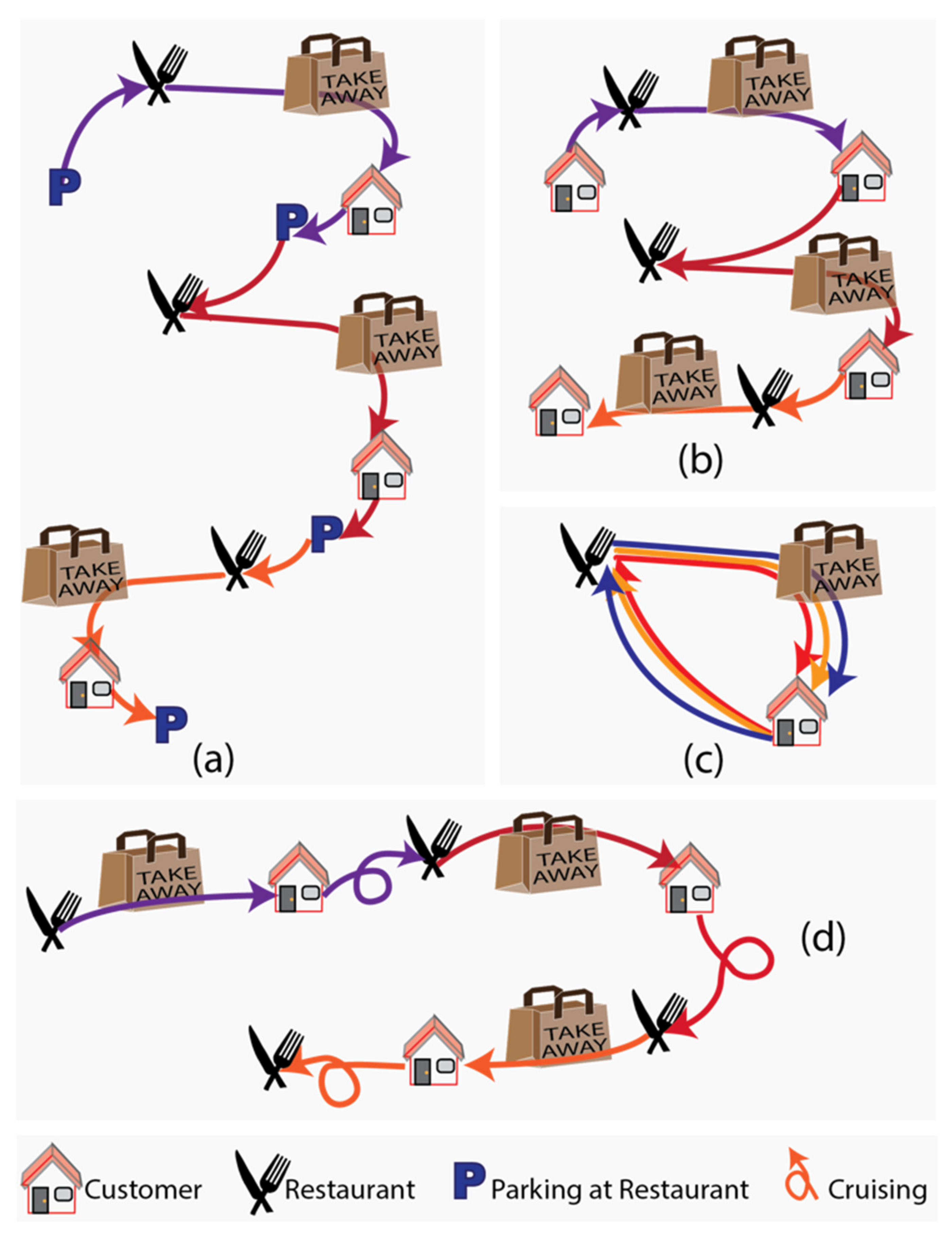
Figure 3 shows the trips involved in the completion of orders for all 4 scenarios. In (a) it is assumed that the SADRs and bicycle couriers are not allowed to wait at the customer’s home for the next order as this would block the footpath or parking spots and couriers should be allowed to wait indoors protected from the weather. SADRs and bicycle couriers travel to and wait at the nearest restaurant after completing an order. This rule increases the VKT and policymakers might decide to forbid additional travel and rather have SADRs wait at the last customer’s address for the next order, which is simulated in (b). In (c) the SADRs and couriers are dedicated to a restaurant and return to the restaurant after an order. In (d) SADRs and bicycle couriers have to pay a parking fee whenever they are standing and therefore keep moving to avoid these charges.
A locally hosted open-source routing machine (OSRM) [62] and the street network from Open Street Map (OSM) [63] have been used to calculate the trip distance and duration of the shortest route. The OSRM pedestrian routing profile has been used for SADRs as they are able to travel on footpaths. The OSRM bicycle profile has been used for bicycle couriers.
To account for the waiting time between two orders, eight average waiting times between two trips have been simulated using eight truncated normal distributions with a mean of i minutes, a lower limit of zero minutes, and an upper limit of i*2 min. The integer i = 1, 2, 4, 8, 16, 32, 64, and 128. All 80 scenarios (10 operating areas by eight average waiting times and 150 orders each) are simulated 100 times each. It is assumed the delivery service runs 24/7.
The handover time has been determined based on the survey and GPS traces of on-demand meal delivery services in the UK. It is defined as the time between arrival at the customer’s address and leaving again including the time required for finding a parking spot and walking to the customer. One responder stated that it usually takes less than 30 s or between 30 s to 1 min to hand over a meal. According to the second responder, it takes in most cases 60–90 s to hand over a meal, but handover times of 0–2 min are common as well. Based on the GPS data of twelve delivery tours (Tour 1: 1:04 h, 16 km; Tour 2: 2:35 h, 22 km; Tour 3: 1:19 h, 21 km; Tour 4: 2:32 h, 30 km; Tour 5: 2:29 h, 34 km; Tour 6: 2:18 h, 31 km; Tour 7: 1:37 h, 24 km; Tour 8: 2:14 h, 33 km; Tour 9: 1:55 h, 27 km; Tour 10: 2:20 h, 27 km; Tour 11: 1:49 h, 20 km, Tour 12: 3:00 h, 43 km) the handover time is on average 73 s (median: 68 s, std: 40 s). These observations are similar to the data from the survey. The time required to pick up a meal from a restaurant varies (mean: 3:14 min, median: 1:05 min, std: 224 s). Approximately 30 % of the meal pickups are longer than 5 min. A reason for this is that it is unknown whether the bicycle courier really picked up a meal at that restaurant or maybe just makes a toilet break or waits in the restaurant for the next order request. Hence, the handover time at the customer’s home has been used as the handover time at restaurants as well. Note: the handover time observed during a study of parcel delivery trips with vans in London [64] is much larger compared with the handover time for on-demand meal delivery observed in this study (mean: 4.1 min, min: 1.6 min, max: 6.8 min, std: 1.2 min). A possible reason could be that customers are expecting a meal delivery, while a parcel might be delivered at a time when the customer is not expecting it. Also, the study in London uses vans, whereas the GPS traces used in this study are from bicycle couriers, who may be able to find a parking spot closer to the customer. It might be debatable whether the handover time of on-demand meal delivery services in UK cities is similar to the handover time observed in NYC. However, the handover time is only affected by the time it takes the customer to answer the door and the time required for the courier to walk from their bicycle to the door and back. Hence, it is not affected by the urban structure, type of streets, traffic and pedestrian volume, etc., and therefore should be relatively similar.

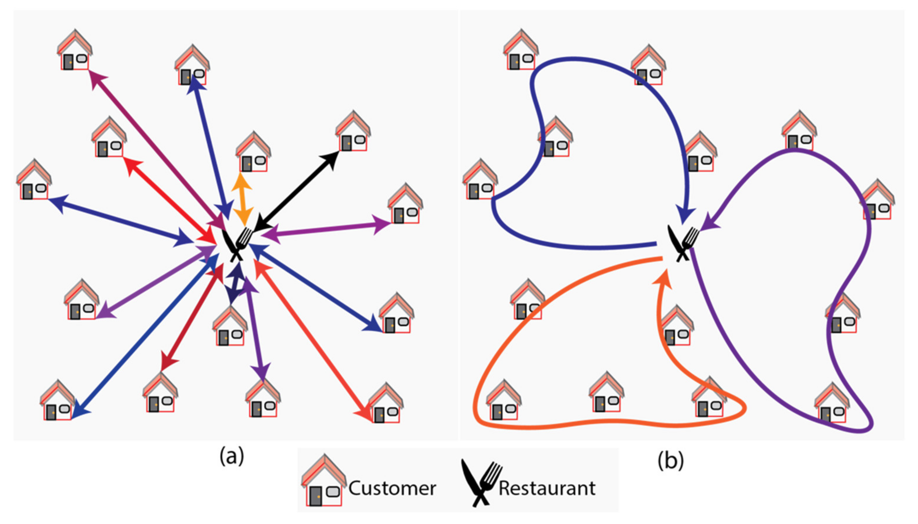
3.3. Study 3: Scheduling: Tour-Based vs. Direct Delivery (Simulation, NYC)

The first simulation assumes that each meal is delivered as a direct delivery tour and each courier serves various restaurants. While this is a common delivery option according to the responders in the previously mentioned survey, both responders state that it is also common for couriers to pick up multiple orders at one restaurant and deliver them in a single tour. According to one of the responders, it is nowadays also possible to first pick up meals from multiple restaurants and then deliver them to multiple customers as a tour.
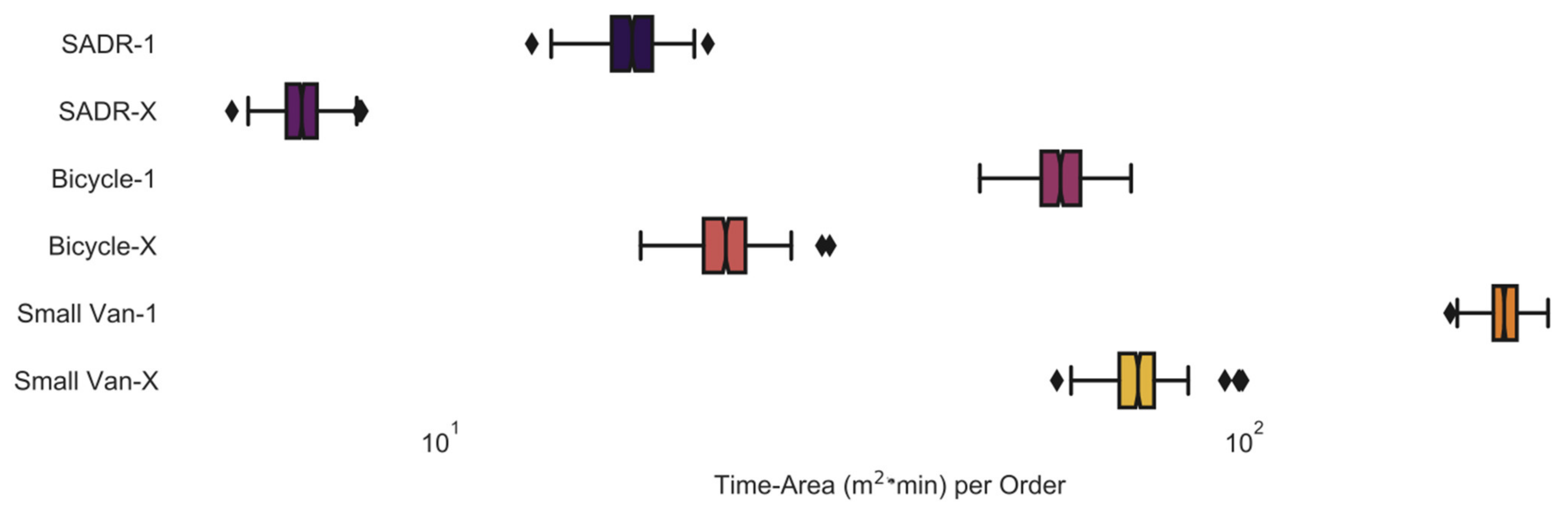
The third study, which compares different scheduling options (i.e., tour-based vs. direct delivery) (Figure 4), uses the same demand for on-demand meal deliveries as the second study. Due to the low speed of SADRs only the smallest operating area is used as it would otherwise be impossible to combine multiple deliveries into one tour and still obey the maximum 30 min delivery time. It is assumed that all vehicles are owned by the restaurant and park at this restaurant after a delivery tour. The closest restaurant to the center of the operating area has been selected. The vehicles are a small van, SADRs, and a bicycle courier. Each mode has been simulated with two different scheduling options; (1) delivering one meal at a time on a first come first serve basis, without any waiting time in between deliveries (SADR-1, Bicycle-1, Small Van-1); and (2) delivering 30 meals during each of the 5 timeslots by a SADR-X, Bicycle-X, or Small Van-X. The roundtrip delivery duration needs to be less than 31.2 min (30 min delivery plus 1.2 min handover time). If a vehicle is not required during a timeslot, it is parked at the restaurant and counts towards the time-area requirements. To ensure an efficient utilization, the vehicles will start with the next tour once the previous tour is finished even if this time is slightly before or after the beginning of the next timeslot.
The following tour scheduling algorithm (1) applies a similar method to the routing algorithm named farthest insertion algorithm:
Input: travel time matrix for all 30 customers and the restaurant
Output: List of customers ordered into tours
  • Select the furthest customer from the restaurant and name it customer A
  • While travel time is <31.2 min and not all customers are served
  • If ‘new customer’ exists delete it from the travel time matrix
  • Add the customer closest to customer A to the list and name it ‘new customer’
  • Calculate the traveling salesman problem for all customers on the list and customer A and the restaurant (roundtrip)
  • If travel time is >31.2 min
  • Delete the ‘new customer’ from the list and place it back into the travel time matrix
  • Calculate the traveling salesman problem for all customers on the list and customer A and the restaurant (roundtrip)
  • Else
  • Calculate the traveling salesman problem for all customers on the list and customer A and the restaurant (roundtrip)
The algorithm selects the furthest customer away first and its neighboring customers, to ensure that the last tour only covers customers close to the restaurant. Like most Traveling salesman solvers, this algorithm will not necessarily find the best tour allocation [65].

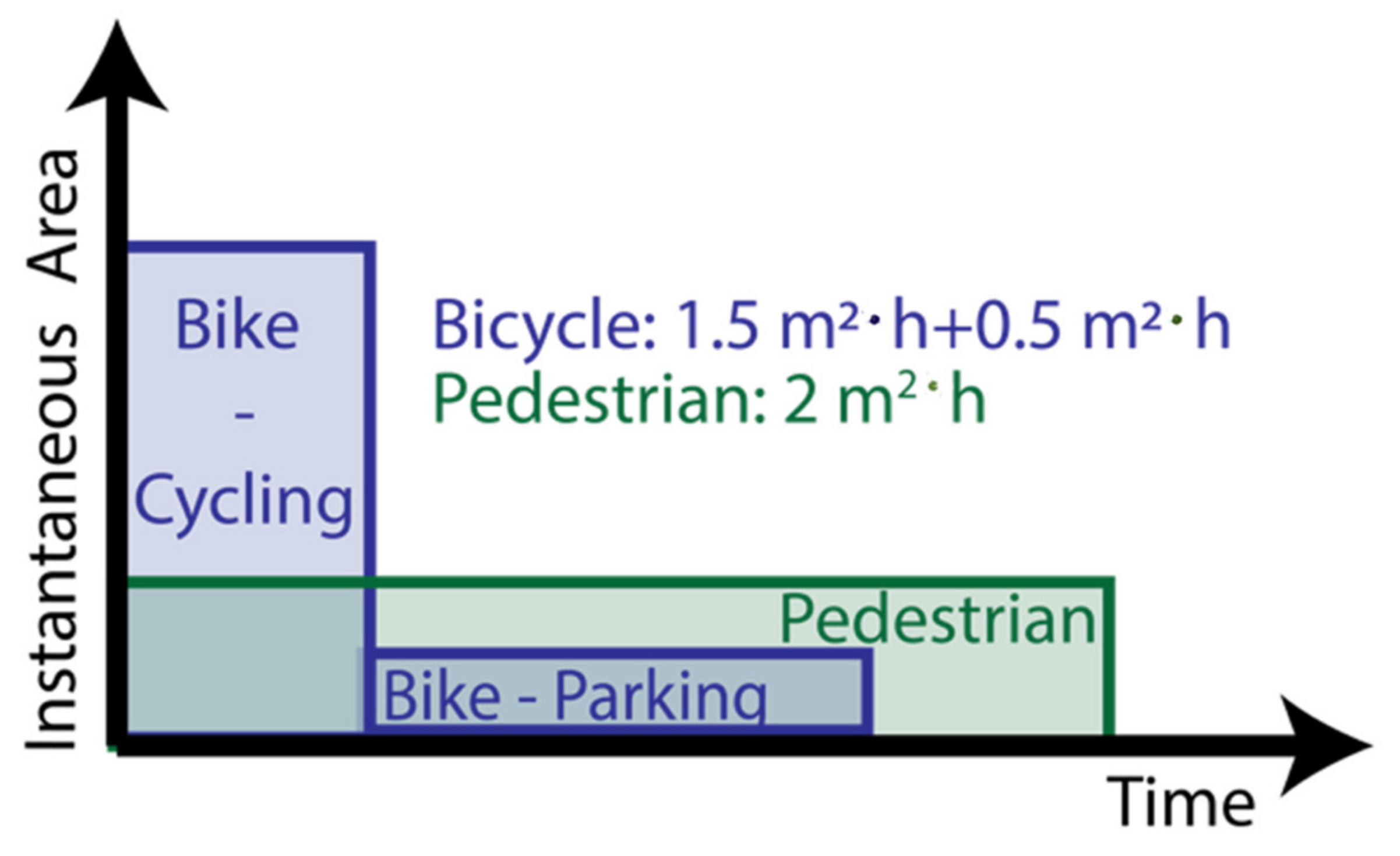
3.4. Time-Area Requirements

As illustrated in Schnieder et al. [23], the time-area concept can consider either the area legally required for safe operation or the share of the provided infrastructure. Using the area legally required for safe operation is more appropriate to the scenarios evaluated in this paper given that bicycles and SADRs do not have a dedicated right-of-way. This means that ground space not used by bicycle couriers or SADRs can be used by other modes of transport (i.e., cars, pedestrians). The equation does not consider the value of land given that considering the value would unfairly impact poorer neighborhoods as stated earlier Schnieder et al. [
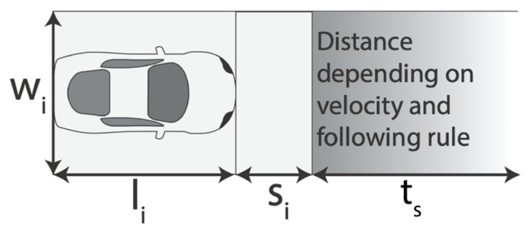
23]. The time-area requirements have been estimated based on the following equation described in Schnieder et al. [23] (Figure 5):
T A i = l i + s i + t s     d i t i     w i     t i ,         i = 1 , 2 , n M T  
Transformed into:
T A i = l i + s i     t i + t s     d i     w i  
where,
  • T A i : Time-area required for trip
  • l i : Length of vehicle
  • s i : Safety distance kept when vehicles are standing
  • t s : Following rule (e.g., 2 s rule)
  • d i : Trip distance
  • t i : Trip duration
  • w i : Width of the lane/right-of-way
For a derivation of the formula, the reader is referred to Schnieder et al. [23]. The safety distance s i is the distance that is maintained between two standing vehicles at a traffic light or while parking parallel to the curb. Without s i the distance kept between vehicles when the velocity is close to 0 would be just a few centimeters. However, the safety distance to the front for bicycles is set to 0 to accommodate the overestimation of the width of the bicycle while standing still (i.e., the dynamic width of a bicycle while cycling is much larger than the width while standing). An explanation of the specifications adopted and comparison with other published research can be found in Schnieder et al. [23]. The size of a typical SADR is based on the Starship delivery robot [66]. The parameter t s is the safe separation distance that is kept between two following vehicles. Given that time-area Equation (2) applies to standing and moving transport units, the order duration is taken as the length of the entire order plus the waiting time until the next order. Table 4 shows the specifications of the time-area requirements for simulations of last-mile delivery vehicles estimated by Schnieder et al. [23] and the resulting instantaneous area requirements. The speed profile refers to the profiles in open-source routing machine (OSRM). Table 5, Table 6 and Table 7 show the resulting instantaneous area requirements.

3.5. Limitations

For simplicity, it is also assumed that the time-area requirements of the bicycle courier when walking the last meters to the customer are included in the time-area requirements of the bicycle.
The utilization is assumed to be the same for shared vehicles and restaurant-owned vehicles. In reality, it is possible that the average utilization is higher for shared vehicles as they serve multiple restaurants which ideally might have their peak demands at different times of the day (e.g., bakeries at breakfast and pizzerias evening/night). Vehicles operated by a single restaurant will have a lower utilization during times outside of the peak demand of the restaurant’s products. By assuming the same utilization for all, the simulation compares the worst case for shared vehicles with the normal case for dedicated vehicles. Otherwise, it could be argued that shared vehicles perform better in simulations due to the assumption that restaurants have their peak demand at different times of the day, which might not be the case in reality. For the same reason, the order of the trips has not been optimized in the simulation and instead a random order of the meal orders has been adopted.

4. Results

4.1. Study 1: GPS Traces (Loughborough/Liverpool)

Table 8 shows the average values for selected key performance parameters. The average shift length is the total duration including any breaks. It is assumed that the bicycle courier is waiting whenever the speed is less than 1.6 km/h. Hence, the waiting time includes the handover time (i.e., time required to hand over meals to the customer including parking the bicycle, walking to the customer and walking back to the bicycle), time to pick up a meal from restaurants, toilet/snack breaks by the courier, brief stops to accept delivery requests, stops to find the correct address if the courier is unable to locate the customer’s address, and stops at traffic lights. The travel duration is the time when the bicycle travels 1.6 km/h or quicker. The share of the waiting time shows the percentage of time when the bicycle courier is stationary. The distance is the distance traveled during the shift. Average speed with and without breaks is calculated by dividing the shift length or the travel duration by the distance traveled. Ascent and descent are the sums of the elevation climbed or descended during the shift. The number of orders is the number of meal deliveries made during a shift.
As can be seen in Table 8, the average of the shift length for the delivery trips in Loughborough during lunch is much smaller given that only half of the delivery tour could be recorded due to battery problems. Most of the shifts were between 2 h and 2.5 h long. The waiting time accounts for around 1/3 of the delivery duration. This result is interesting given that the handover time alone is 62 % of the delivery duration for parcel deliveries in London [64]. Only the average share of the waiting time for Loughborough-Dinner is relatively large (i.e., 51 %). The data from Loughborough should be interpreted carefully given that it is based on 1 or 2 trips and only part of the shift has been recorded due to battery problems. The data from Liverpool are full shifts and based on 4 or 5 trips. The average travel duration per meal delivery is 15–17 min and the average delivery duration per meal delivery including waiting time is 22–30 min. The average distance per shift is around 30 km in Liverpool and around 5 km per order. The courier ascends by a total of around 95 m in Loughborough and around 240 m in Liverpool. The average speed with waiting time is less than 15 km/h and close to 20 km without waiting time. The average number of orders per shift is 6 in Liverpool.
The time-area requirements per order for every shift are shown in Figure 6. The median of the time-area requirements for Liverpool is 322 m2·min per order for lunch and 292 m2·min per order for dinner. Based on the limited data available for Loughborough, the average time-area requirements per order is 361 m2·min for lunch time.

4.2. Study 2: Policy and Operating Strategies (Simulation, NYC)

4.2.1. Key Performance Indicators

The travel duration from the restaurant to the customer including the handover time is shown in Figure 7. Given that SADRs typically travel at walking speed [66], they can only operate in a small operating area if they are required to deliver hot food. In the UK it is advised to deliver hot food within 30 min (i.e., [67,68]). This rule would be broken by a few delivery trips in operating area 3 (Figure 7) and larger. Under the 30-min constraint bicycles travel quickly enough to be able to deliver hot food as far as operating area 5 (Figure 7). The larger operating areas are included in the study given that the delivery time of chilled food is longer or heated storage could keep food hot for longer.
Figure 8 shows the distance travelled to fulfill a single order. Overall, the distance per order is similar for the six delivery options. The distance covered by bicycles is slightly larger (16 % operating area 1, reduced to 3 % in operating area 10) given that SADRs travel on the footpath and are not affected by one-way streets and other routing constraints. The maximum battery range of SADRs (e.g., [66]) is too short for most trips in operating area 3 or larger. This problem would be amplified were it is not possible to recharge the delivery robots at every restaurant. The difference between restaurant owned (i.e., dedicated) vehicles and shared (a) and shared (b) is around 10 % in operating area 1 and reduces quickly to less than 1 % for operating area 7 or larger.
The time required to fulfill one order is longer for SADRs than for bicycle couriers (70 % in operating area 1, increasing to 2.5-fold in operating area 10) due to the slower speed (Figure 9). The difference in the travel duration between shared and dedicated vehicles is rather small, which is similar to the travel distance.
Figure 10 shows the increase in order duration and distance assuming that shared bicycles parking at the customer is 100 % (i.e., Bicycle Shared (b)). The average delivery duration of SADR Shared (b) is 1.7 (operating area 1) to 2.5 times (operating area 10) longer than for Bicycle Shared (b). The difference in the duration between shared vehicles parking at restaurants (a) and restaurant owned vehicles (i.e., dedicated vehicles (c)) is less than 1 % for both modes of transport.
The travel distance of SADR Shared (b) is between 15 % smaller in operating area 1 (19 % for SADRs) and 3 % smaller in operating area 10 (2 % for SADRs) than Bicycle Shared (b). The absolute increase in travel distance is less than 500 m in all cases. The trip distance for SADRs is only 85 % (operating area 1) of the trip distance of bicycle couriers given that SADRs are not affected by one-way streets etc. The effect reduces when the trip distance is increasing.

4.2.2. Time-Area Requirements

The time-area requirements are illustrated in Figure 11. Restaurant-owned SADRs have a less than 1 % higher time-area requirement compared with SADRs parking at customers. Requiring SADRs to park at a restaurant (a) increases the time-area requirements by 1 % to 19 %. The percentage increases with the operating area size and decreases with the waiting time between trips. This is due to the waiting time requiring the same time-area regardless of the parking location. The time-area requirement of bicycles is around 2.7 to 3.6 times larger compared to SADRs. The difference reduces when the operating area size increases, or the waiting time reduces. While keeping moving to avoid parking charges might be unrealistic for bicycle couriers, it is an attractive option for autonomous vehicles as driving is usually cheaper than parking charges [16]. The time-area requirement of SADRs traveling at walking speed is twice as high as the time-area requirements of standing SADRs. If parking policy (d: shared vehicles cruising around instead of parking) is implemented, the time-area requirements of SADRs increases by up to 82 % (wait 128 min, Operating Area 1) compared to SADR Shared (b).

4.2.3. Sensitivity Analysis

Figure 12 shows the sensitivity analysis. On the left side in Figure 12, the average waiting time between trips is increased while the operating area is always operating area 5. On the right side in Figure 12, the operating area size is increased while the waiting time is constant at 32 min. The length l i , safety distance s i , width w i , following rule t s , travel time t i (i.e., handover time + driving time), and travel distance d i   have been increased by 20 % and the increase in the time-area requirements has been calculated. In all cases, an increase in the width of a vehicle increases the time-area requirement correspondingly. The graphs for bicycles and SADRs are similar apart from the effect of an increased travel distance being lower for SADRs and the effect of an increase in the safety distance and travel time being larger for SADRs. As can be seen in Equation (1), an increase in the travel time and following rule has the same effect as both factors are multiplied by each other. The difference in the sensitivity between operating strategies and parking policies is negligible.

4.3. Study 3: Scheduling: Tour-Based vs. Direct Delivery (Simulation, NYC)

The number of vehicles required for each of the 500 delivery slots (five slots per day over 100 days) is relatively constant for the tour-based delivery simulation: Either two small vans (maximum three) or three bicycles (maximum four) are required for almost all of the 500 delivery slots. In most cases, four or five SADRs are required for each delivery slot due to the low speed. Only three delivery slots require three SADRs. The simulation always assumes that either five SADRs, four bicycle couriers, or three small vans are used to deliver the meals given that this is the maximum number of vehicles required. Vehicles are parked at the restaurant during the slots they are not required and count towards the time-area requirement.
Figure 13 compares the time-area requirements for all three modes of transport and tour scheduling options. Combining multiple deliveries into one tour reduces the time-area requirement by 60%–65%. Even if SADRs would only be able to deliver one meal per tour (17 m2·min), the required time-area would still be 23% smaller than that of a bicycle courier which delivers multiple meals in one tour. Policymakers should discourage the use of cars to deliver meals in cities given that even a small van requires three times as much time-area compared to a bicycle.
Figure 14 shows the sensitivity analysis. Each factor listed on the right in the figure is increased by 20%. The sensitivity is relatively similar across all delivery options and modes of transport.
As in study 2, an increase in the safety distance s i has the smallest effect (i.e., <2.4%) and an increase in the width w i has the largest effect on the time-area requirements (i.e., 20%). Increasing the length l i of the vehicle or travel time t i by 20% increases the time-area requirements by 5.2–9.4% and 5.8–11.5%, respectively. Increasing the following rule t s or travel distance d i increases the time-area requirements by 8.5–14.2%.

5. Discussion

Regulating delivery services using autonomous vehicles is a challenge that will soon be faced by policymakers. The environmental performance of urban freight is in most cases focused on emissions [19], which neglects the importance of allocating land effectively. Given that every square meter devoted to streets is lost for other purposes such as housing or parks [23], reducing land consumption [20] as well as increasing the land use efficiency [21] is increasingly a key objective for policymakers.
The time-area concept is especially useful for this aim as it can be used to compare modes of transport that have different sizes and velocities, and it combines the requirements of moving and standing transport units in one metric. The latter makes the time-area concept especially useful for autonomous vehicles, which can avoid parking charges by continuing to drive.
This paper has applied the time-area concept to simulations of on-demand meal delivery services in NYC as well as to GPS traces of real on-demand meal delivery tours in the UK. Different vehicles (i.e., SADRs and bicycle couriers, small delivery vans), using different operating strategies (i.e., shared vs. dedicated fleets), following various parking policies (i.e., parking at restaurants, parking at the customer’s home, and no parking policies), and two scheduling options (i.e., direct vs. tour-based delivery) are simulated and evaluated.
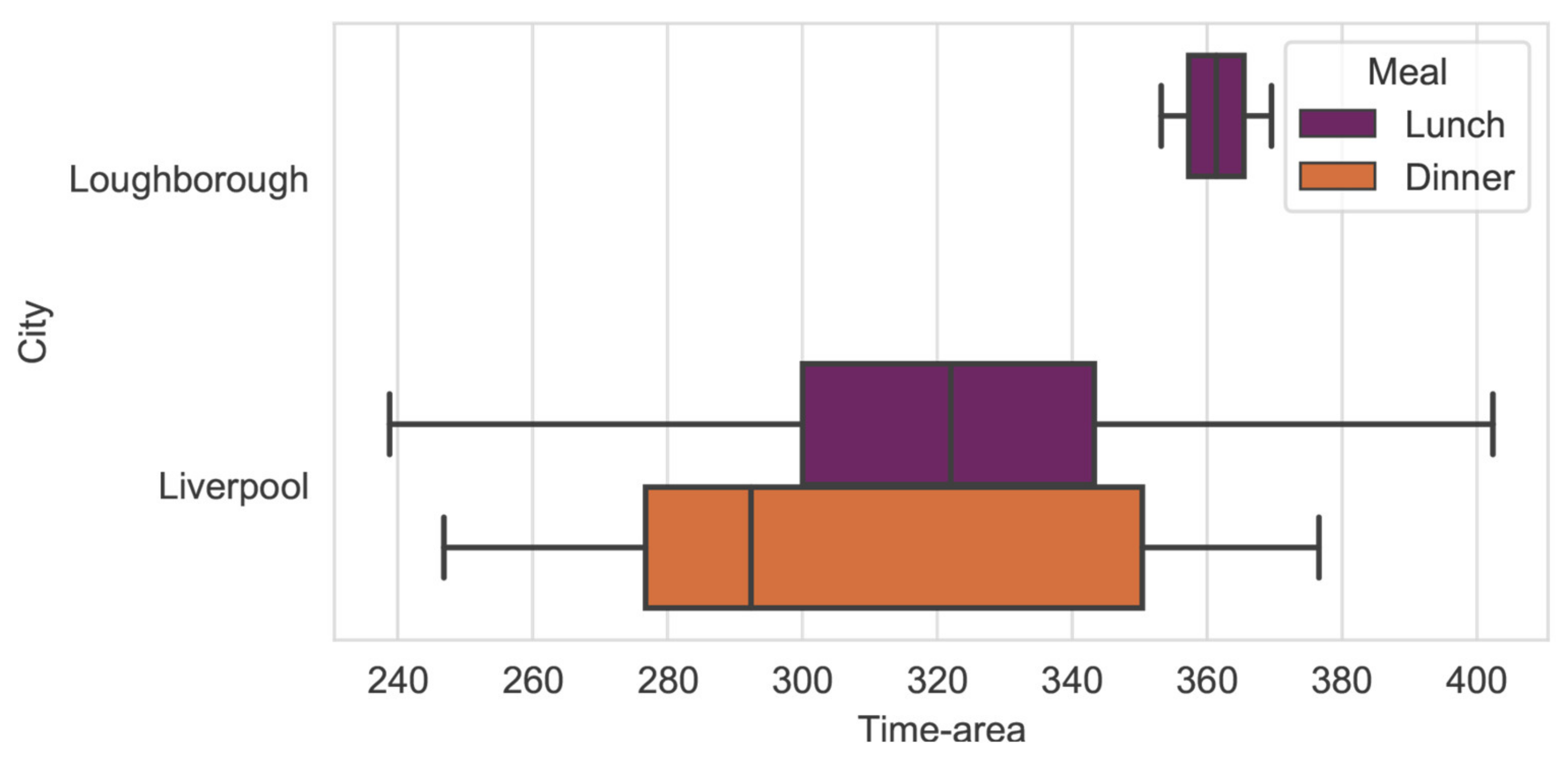
The GPS traces (Loughborough and Liverpool) show that the on-demand meal delivery bicycle is only stationery for around 30% of the time. This result is interesting given that parcel delivery vans are stationary for 62% of the delivery time in London [64]. It would be worth investigating the reasons for this. Doing so enables companies to identify options to increase the efficiency of last-mile delivery by reducing handover time. Possible reasons include (i) bicycle couriers may be able to park closer to the customer than delivery vans, (ii) high-rise buildings in London may make deliveries more difficult, (iii) parcel delivery locations may be closer together than the on-demand meal delivery location, or (iv) a meal delivery customer might be more aware of the delivery time point than a customer waiting for a parcel.
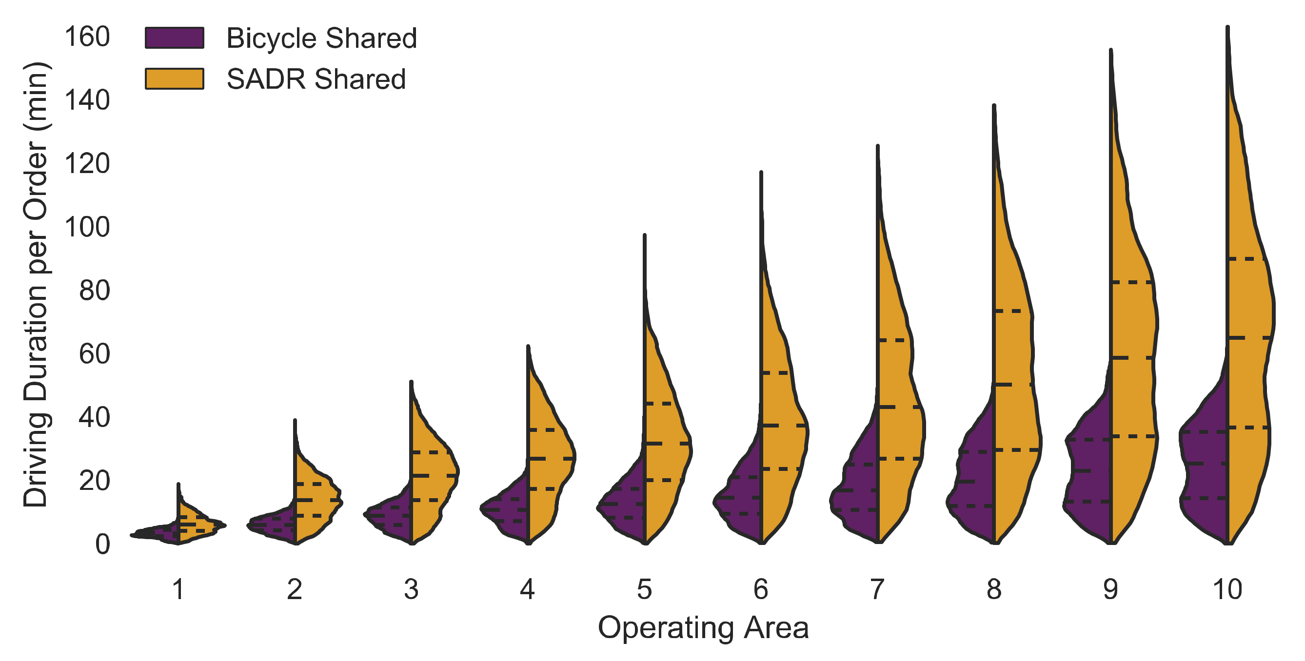
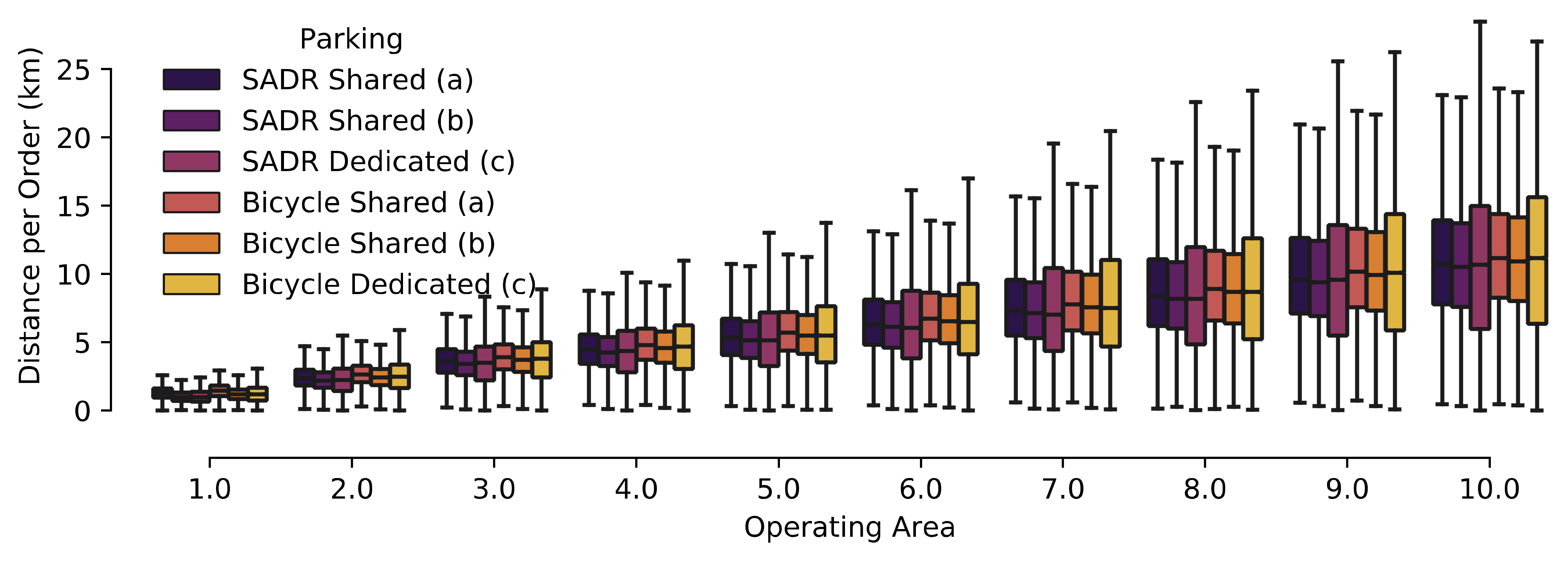
When comparing the simulation of study 2 for NYC with the results from the GPS traces from Loughborough and Liverpool, it can be seen that the key-performance indicators based on GPS traces and operating area 5 (simulation) with less than 16 min wait between orders are similar (e.g., distance per order is around 5 km). Also, the time-area requirements are similar.
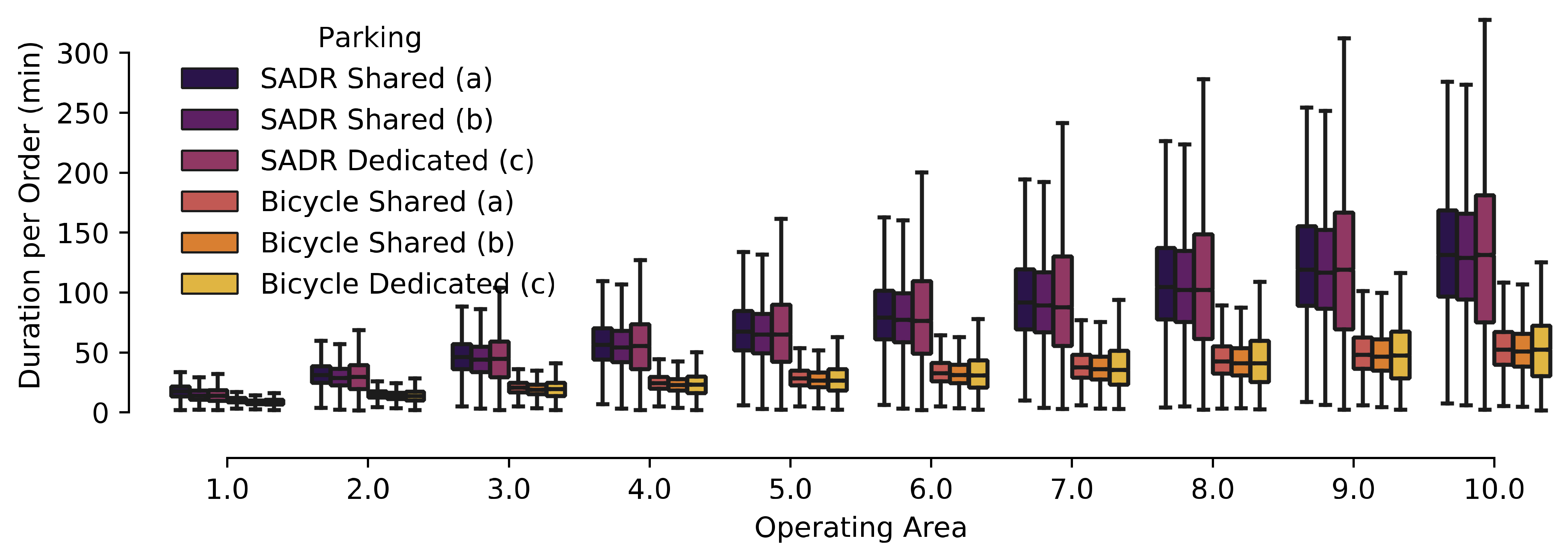
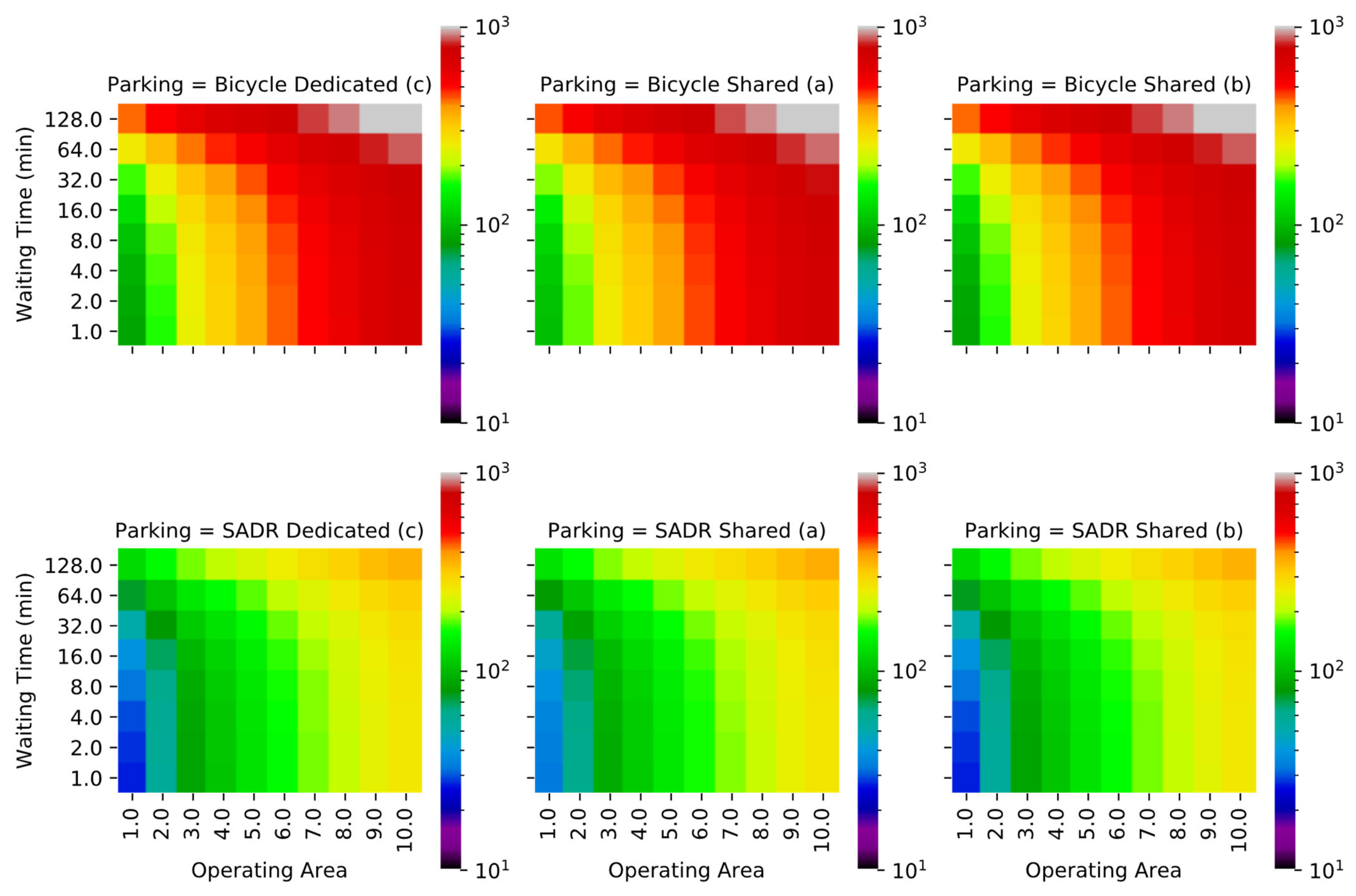
The results of the second study show that SADRs can only operate in very small operating areas due to their current safe operating speeds being too slow to deliver hot meals within the recommended time frame in large operating areas. The area-time requirements of SADRs are around half of the time-area requirements for cycling couriers. This result is another argument in favor of the ‘15-min city’. The ’15-min city’ refers to a city structure where all residents can walk or ride a bike to reach daily errands (i.e., work, school, shopping) within 15 min [69]. The ‘15-min city’ not only enables people to meet their mobility needs, it also allows for the implementation and use of innovative forms of last-mile delivery. Completely segregated cities or residential suburbs, that don’t have any restaurants, are not a good fit for SADRs.
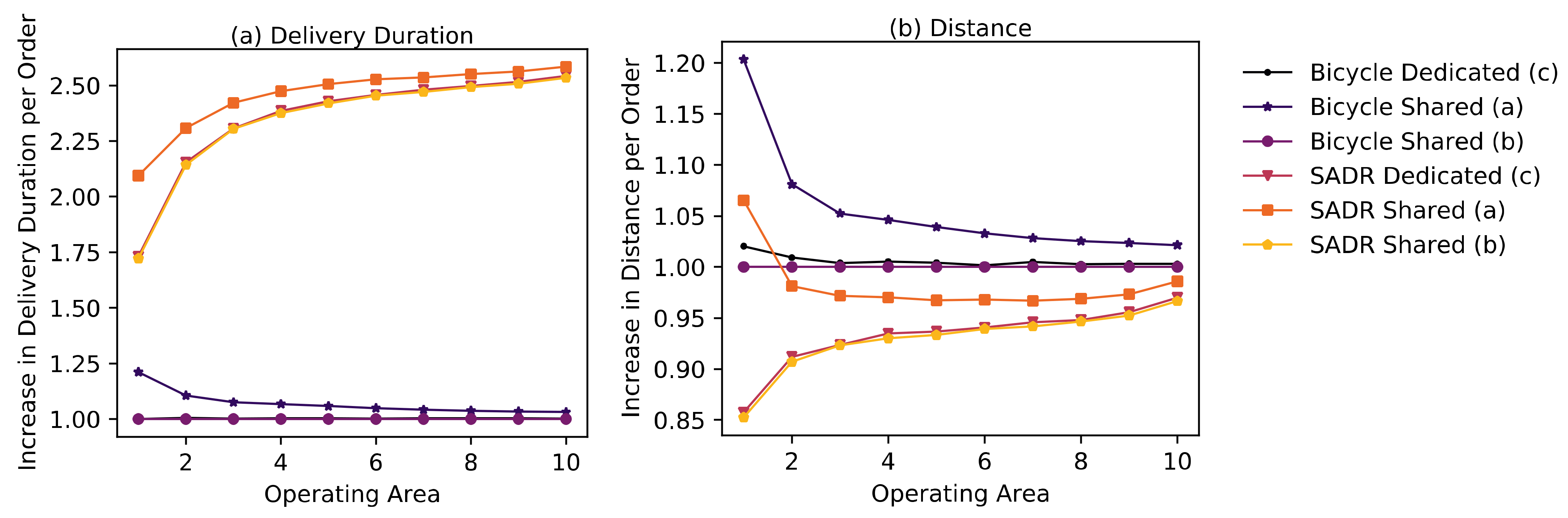
Operating strategy changes (i.e., shared vs. restaurant owned), and two of the parking policies (parking at restaurant vs. parking at customer), have only small effects on the time-area requirements.
Under no circumstances should policymakers disincentivize parking for autonomous delivery vehicles (e.g., implementing parking charges) as this would incentivize autonomous vehicles to drive around instead of parking. Doing so increases the time-area requirements by 2–5 times assuming average speeds in cities. Thus, parking charges are as counterproductive for SADRs as they are for autonomous passenger vehicles [16]. A better strategy would be to use a time-area based road pricing method. When cars are the main mode of transport, charging fees per trip is reasonable (i.e., parking charges). However, the shape, size, and average speed can vary between autonomous vehicles, micromobility, and cycling. Consequently, a per vehicle charge would not be fair. The time-area concept would allow policymakers to define a fair charge for each transport activity exactly based on the ground area and time they occupy. By doing so policymakers would incentivize modes of transport that use land more effectively, which maximizes sustainability.
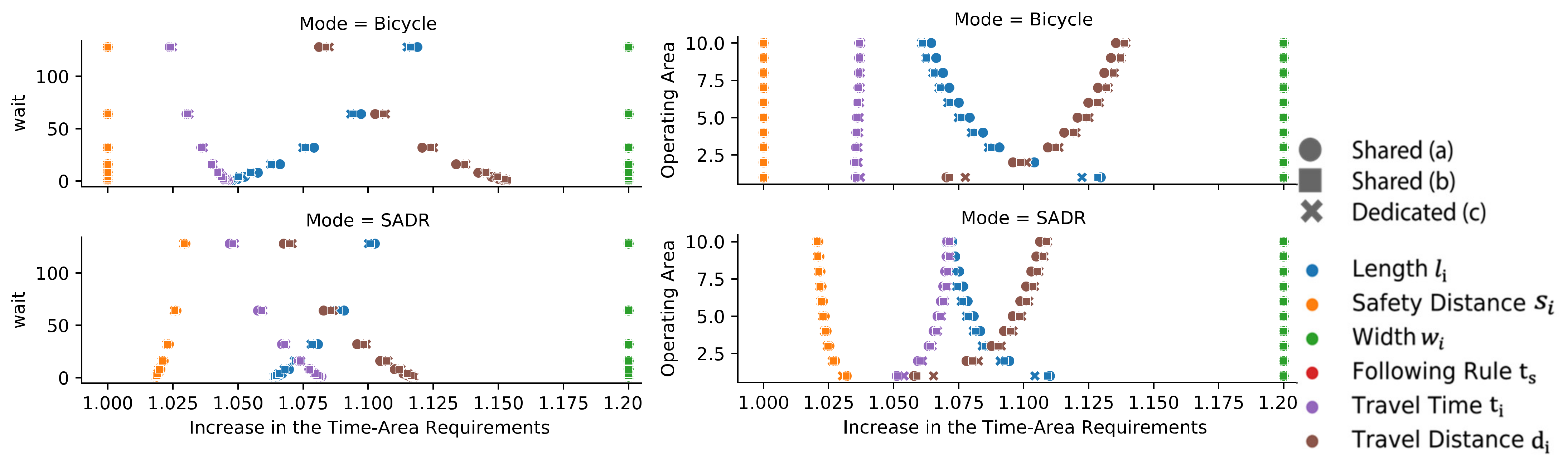
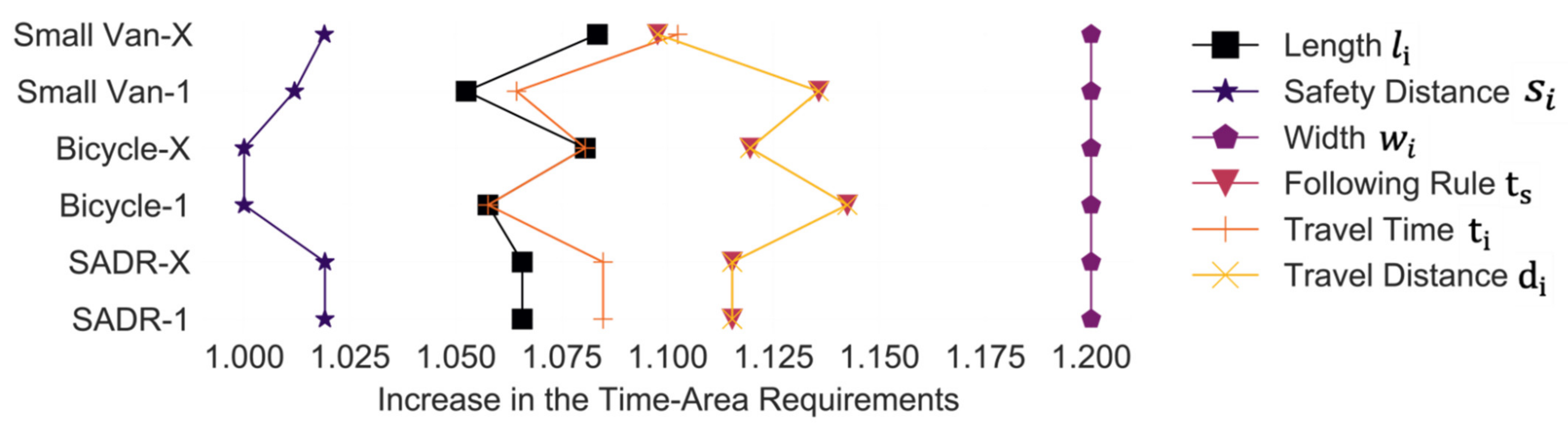
Increasing the travel time (i.e., reducing the travel speed) increases the time-area requirements only by a fraction of this increase, as seen in the sensitivity analysis. The same applies to increasing the vehicle length. If the vehicle width is increased, the time-area requirements increase by the same percentage.
Combining multiple deliveries into one tour reduces the time-area requirement by 60 %-65 %, when using SADRs, bicycles or small vans (study 3). This highlights the benefits of aggregator platforms and sharing resources (i.e., delivery vehicles). Instead of having multiple providers who own, run and optimize their own fleet of vehicles, it would be better for them to collaborate to take advantage of economies of scale by increasing the likelihood that multiple customers live close together.
As previously stated, utilization is the same for shared vehicles and restaurant-owned vehicles in the simulation, even though shared vehicles could achieve a higher utilization if they serve restaurants which have their peak demands at different times of the day. A bakery might have their peak demand at breakfast and pizzerias in the evening. Nevertheless, it has been assumed that the utilization is the same to ensure that shared vehicles are not only performing better due to the assumed higher utilization, which might not be the case in reality. The order of the trips has not been optimized for the same reason. Nevertheless, a follow up study could investigate whether a utilization increase could realistically be achieved (using real data), and the effect of this increase on the time-area requirements.
The differences between the time-area requirements of each mode of transport are clearly visible in study 3: A SADR delivering only one meal at a time has a 23% smaller time-area requirement than a bicycle courier delivering multiple meals per tour. This again highlights the importance of the economics of scale, given that bicycle couriers can achieve similar time-area requirements to a SADR if they deliver multiple meals per tour.
A small van requires 3 times as much time-area compared to a bicycle assuming that both deliver multiple meals per tour. Therefore, policymakers should discourage the use of cars to deliver meals in cities as well as build the city so that delivery by bicycle or SADR is easily possible.

6. Conclusions

The paper evaluates the land consumption of on-demand meal delivery services such as UberEATS and Deliveroo based on the time-area concept. The time-area concept measures the area required for a transport activity and the duration for which it is occupied. The contribution of the paper is twofold: First, the paper calculates the time-area requirements of GPS traces of on-demand meal delivery tours in Liverpool and Loughborough (UK). Second, on-demand meal delivery trips using bicycle couriers and SADRs are simulated for NYC. Various operating strategies (i.e., shared fleets and fleets operated by restaurants), parking policies (i.e., parking at the restaurant, parking at the customer or no parking), and scheduling (i.e., one meal per vehicle, multiple meals per vehicle) are simulated.
The dataset of GPS traces includes 25 h and 327 km worth of data for two cities in the UK. Most of the data has been recorded in Liverpool. The Loughborough dataset is, with 5 h and 59 km, relatively small and does not, in contrast to the Liverpool data, include full delivery trips. The results show that the time-area requirement is around 300 m2·min per order.
The simulations show that SADRs are only an option for small operating areas, but their time-area requirements are only around half of that of bicycle couriers. If bicycle couriers deliver multiple meals per tour while SADRs deliver one meal at a time, SADRs still require 23% less time-area. Delivering meals by small vans can never be recommended.

Author Contributions

Conceptualization, M.S.; data curation, M.S.; formal analysis, M.S.; investigation, M.S.; methodology, M.S.; resources, A.W.; software, M.S.; supervision, C.H. and A.W.; validation, M.S., C.H. and A.W.; visualization, M.S.; writing—original draft, M.S.; writing—review and editing, M.S., C.H. and A.W. All authors have read and agreed to the published version of the manuscript.

Funding

The authors gratefully acknowledge the financial support of the Engineering and Physical Sciences Research Council (EPSRC) Centre for Doctoral Training in Embedded Intelligence under grant reference EP/L014998/1 and Ford Motor company for their support and input to this research.

Institutional Review Board Statement

The survey has been reviewed and deemed appropriate by the Ethics Review Sub-Committee at Loughborough University (2021-5405-4323).

Informed Consent Statement

Informed consent was obtained from all subjects involved in the study.

Data Availability Statement

[Address Points] Department of Information Technology and Telecommunications (DoITT). NYC Address Points|NYC Open Data. 2019. Available online: https://data.cityofnewyork.us/City-Government/NYC-Address-Points/g6pj-hd8k (accessed on 5 February 2019). [Population density] Department of City Planning (DCP). Census Demographics at the Neighborhood Tabulation Area (NTA) Level|NYC Open Data. 2018. Available online: https://data.cityofnewyork.us/City-Government/Census-Demographics-at-the-Neighborhood-Tabulation/rnsn-acs2 (accessed on 17 April 2019). [Meal delivery data] Department of Transportation. Citywide Mobility Survey—Main Survey|NYC Open Data. 2017. Available online: https://data.cityofnewyork.us/Transportation/Citywide-Mobility-Survey-Main-Survey/dd6w-hnq9 (accessed on 13 February 2019). [Bike sharing stations] Motivate. Citi Bike System Data|Citi Bike NYC. 2019. Available online: https://www.citibikenyc.com/system-data (accessed on 8 May 2019).

Acknowledgments

Map data copyrighted OpenStreetMap contributors and available from https://www.openstreetmap.org (accessed on 1 May 2019). The GPS traces of on-demand meal delivery trips were kindly provided by Ben Emsley.

Conflicts of Interest

The authors declare no conflict of interest. The funders had no role in the design of the study; in the collection, analyses, or interpretation of data; in the writing of the manuscript, or in the decision to publish the results.

References

  1. Kin, B.; Verlinde, S.; Macharis, C. Sustainable urban freight transport in megacities in emerging markets. Sustain. Cities Soc. 2017, 32, 31–41. [Google Scholar] [CrossRef]
  2. Le, T.V.; Stathopoulos, A.; van Woensel, T.; Ukkusuri, S.V. Supply, demand, operations, and management of crowd-shipping services: A review and empirical evidence. Transp. Res. Part C Emerg. Technol. 2019, 103, 83–103. [Google Scholar] [CrossRef]
  3. Statista Research & Analysis. eServices Report 2020-Online Food Delivery. 2020. Available online: https://0-www-statista-com.brum.beds.ac.uk/study/40457/food-delivery/ (accessed on 19 May 2021).
  4. Yildiz, B.; Savelsbergh, M. Service and capacity planning in crowd-sourced delivery. Transp. Res. Part C Emerg. Technol. 2019, 100, 177–199. [Google Scholar] [CrossRef]
  5. Jennings, D.; Figliozzi, M. Study of Sidewalk Autonomous Delivery Robots and Their Potential Impacts on Freight Efficiency and Travel. Transp. Res. Rec. 2019, 2673, 317–326. [Google Scholar] [CrossRef] [Green Version]
  6. Fanti, M.P.; Mangini, A.M.; Roccotelli, M.; Silvestri, B. Hospital Drugs Distribution with Autonomous Robot Vehicles. In Proceedings of the 2020 IEEE 16th International Conference on Automation Science and Engineering (CASE), Hong Kong, China, 20–21 August 2020; Institute of Electrical and Electronics Engineers (IEEE): Piscataway, NJ, USA, 2021; pp. 1025–1030. [Google Scholar]
  7. Cheong, W.S.; Kamarulzaman, S.F.; Rahman, M.A. Implementation of Robot Operating System in Smart Garbage Bin Robot with Obstacle Avoidance System. In Proceedings of the 2020 Emerging Technology in Computing, Communication and Electronics (ETCCE), Dhaka, Bangladesh, 21–22 Decembre 2020; Institute of Electrical and Electronics Engineers (IEEE): Piscataway, NJ, USA, 2021; pp. 1–6. [Google Scholar]
  8. Buchegger, A.; Lassnig, K.; Loigge, S.; Mühlbacher, C.; Steinbauer, G. An Autonomous Vehicle for Parcel Delivery in Urban Areas. In Proceedings of the 2018 21st International Conference on Intelligent Transportation Systems (ITSC), Maui, HI, USA, 4–7 November 2018; Institute of Electrical and Electronics Engineers (IEEE): Piscataway, NJ, USA, 2019; pp. 2961–2967. [Google Scholar]
  9. Figliozzi, M.; Jennings, D. Autonomous delivery robots and their potential impacts on urban freight energy consumption and emissions. Transp. Res. Procedia 2020, 46, 21–28. [Google Scholar] [CrossRef]
  10. Figliozzi, M.A. Carbon emissions reductions in last mile and grocery deliveries utilizing air and ground autonomous vehicles. Transp. Res. Part D Transp. Environ. 2020, 85, 1–12. [Google Scholar] [CrossRef] [PubMed]
  11. Villaronga, E.F.; Golia, A.J. Robots, standards and the law: Rivalries between private standards and public policymaking for robot governance RR. Comput. Law Secur. Rev. Int. J. Technol. Law Pract. 2019, 35, 129–144. [Google Scholar] [CrossRef]
  12. Brown, A.; Klein, N.J.; Thigpen, C.; Williams, N. Impeding access: The frequency and characteristics of improper scooter, bike, and car parking. Transp. Res. Interdiscip. Perspect. 2020, 4, 100099. [Google Scholar] [CrossRef]
  13. Zhang, Y.; Lin, D.; Mi, Z. Electric fence planning for dockless bike-sharing services. J. Clean. Prod. 2019, 206, 383–393. [Google Scholar] [CrossRef]
  14. Su, D.; Wang, Y.; Yang, N.; Wang, X. Promoting considerate parking behavior in dockless bike-sharing: An experimental study. Transp. Res. Part A Policy Pract. 2020, 140, 153–165. [Google Scholar] [CrossRef]
  15. Laa, B.; Emberger, G. Bike sharing: Regulatory options for conflicting interests—Case study Vienna. Transp. Policy 2020, 98, 148–157. [Google Scholar] [CrossRef]
  16. Millard-Ball, A. The autonomous vehicle parking problem. Transp. Policy 2019, 75, 99–108. [Google Scholar] [CrossRef]
  17. Shi, J.G.; Si, H.; Wu, G.; Su, Y.; Lan, J. Critical factors to achieve dockless bike-sharing sustainability in China: A stakeholder-oriented network perspective. Sustainability 2018, 10, 2090. [Google Scholar] [CrossRef] [Green Version]
  18. Comi, A.; Schiraldi, M.M.; Buttarazzi, B. Smart urban freight transport: Tools for planning and optimising delivery operations. Simul. Model. Pract. Theory 2018, 88, 48–61. [Google Scholar] [CrossRef]
  19. Muñoz-Villamizar, A.; Santos, J.; Montoya-Torres, J.; Velázquez-Martínez, J. Measuring environmental performance of urban freight transport systems: A case study. Sustain. Cities Soc. 2020, 52, 101844. [Google Scholar] [CrossRef]
  20. Sapena, M.; Ruiz, L.Á. Analysis of land use/land cover spatio-temporal metrics and population dynamics for urban growth characterization. Comput. Environ. Urban. Syst. 2019, 73, 27–39. [Google Scholar] [CrossRef]
  21. Zitti, M.; Ferrara, C.; Perini, L.; Carlucci, M.; Salvati, L. Long-term urban growth and land use efficiency in Southern Europe: Implications for sustainable land management. Sustainability 2015, 7, 3359–3385. [Google Scholar] [CrossRef] [Green Version]
  22. Manville, M.; Shoup, D. Parking, People, and Cities. J. Urban. Plan. Dev. 2005, 131, 246–257. [Google Scholar] [CrossRef] [Green Version]
  23. Schnieder, M.; Hinde, C.; West, A. Review and Development of a Land Consumption Evaluation Method Based on the Time-Area Concept of Last Mile Delivery Using Real Delivery Trip Data. Sustainability 2020, 12, 10626. [Google Scholar] [CrossRef]
  24. Bruun, E.C. Calculation and evaluation of the time-area parameter for different transportation modes. Ph.D. Thesis, University of Pennsylvania, ProQuest Dissertations Publishing, Philadelphia, PA, USA, 1992. [Google Scholar]
  25. Zhou, J.; Chang, S.; Ma, W.; Wang, D. An unbalance-based evaluation framework on urban resources and environment carrying capacity. Sustain. Cities Soc. 2021, 72, 103019. [Google Scholar] [CrossRef]
  26. Graymore, M.L.M.; Sipe, N.G.; Rickson, R.E. Sustaining Human Carrying Capacity: A tool for regional sustainability assessment. Ecol. Econ. 2010, 69, 459–468. [Google Scholar] [CrossRef]
  27. Zheng, N.; Geroliminis, N. On the distribution of urban road space for multimodal congested networks. Transp. Res. Part B Methodol. 2013, 57, 326–341. [Google Scholar] [CrossRef] [Green Version]
  28. Oh, K.; Jeong, Y.; Lee, D.; Lee, W.; Choi, J. Determining development density using the Urban Carrying Capacity Assessment System. Landsc. Urban. Plan. 2005, 73, 1–15. [Google Scholar] [CrossRef]
  29. Gössling, S. Urban transport justice. J. Transp. Geogr. 2016, 54, 1–9. [Google Scholar] [CrossRef]
  30. Guzman, L.A.; Oviedo, D.; Arellana, J.; Cantillo-García, V. Buying a car and the street: Transport justice and urban space distribution. Transp. Res. Part D Transp. Environ. 2021, 95, 102860. [Google Scholar] [CrossRef]
  31. Verhoef, E. External effects and social costs of road transport. Transp. Res. Part A 1994, 28, 273–287. [Google Scholar] [CrossRef]
  32. Euchi, J.; Kallel, A. Internalization of external congestion and CO2 emissions costs related to road transport: The case of Tunisia. Renew. Sustain. Energy Rev. 2021, 142, 110858. [Google Scholar] [CrossRef]
  33. Page, M.J.; McKenzie, J.E.; Bossuyt, P.M.; Boutron, I.; Hoffmann, T.C.; Mulrow, C.D.; Shamseer, L.; Tetzlaff, J.M.; Akl, E.A.; Brennan, S.E.; et al. The PRISMA 2020 statement: An updated guideline for reporting systematic reviews. BMJ 2021, 372, n71. [Google Scholar] [CrossRef]
  34. Starczewski, J. Analysis of Transport Process’ Costs with Use Various Technologies in Terms of Last Mile Delivery Problem. Adv. Intell. Syst. Comput. 2020, 1032, 401–410. [Google Scholar]
  35. Mommens, K.; Rai, H.B.; van Lier, T.; Macharis, C. Delivery to homes or collection points? A sustainability analysis for urban, urbanised and rural areas in Belgium. J. Transp. Geogr. 2021, 94, 103095. [Google Scholar] [CrossRef]
  36. Verlinden, T.; van de Voorde, E.; Dewulf, W.H.R.C. logistics and European medieval structured cities: A search for cost generators. Transp. Policy 2020, 99, 419–429. [Google Scholar] [CrossRef]
  37. Veličković, M.; Stojanović, Đ.; Nikoličić, S.; Maslarić, M. Different Urban Consolidation Centre Scenarios: Impact on External Costs of Last-Mile Deliveries. Transport 2017, 33, 948–958. [Google Scholar] [CrossRef] [Green Version]
  38. Villa, R.; Monzón, A. A metro-based system as sustainable alternative for urban logistics in the era of e-commerce. Sustainability 2021, 13, 4479. [Google Scholar] [CrossRef]
  39. Leyerer, M.; Oliver, M.; Maximilian, S. Urban Parcel Delivery; Springer: Berlin/Heidelberg, Germany, 2019; Volume 7. [Google Scholar]
  40. Ranieri, L.; Digiesi, S.; Silvestri, B.; Roccotelli, M. A review of last mile logistics innovations in an externalities cost reduction vision. Sustainability 2018, 10, 782. [Google Scholar] [CrossRef] [Green Version]
  41. van Essen, H.; van Wijngaarden, L.; Schroten, A.; Sutter, D.; Bieler, C.; Maffii, S.; Brambilla, M.; Fiorello, D.; Fermi, F.; Parolin, R.; et al. Handbook on the External Costs of Transport, Version 2019; CE Delft: Delft, The Netherlands, 2019. [Google Scholar]
  42. Maibach, M.; Schreyer, C.; Sutter, D.; van Essen, H.P.; Boon, B.H.; Smokers, R.; Schroten, A.; Doll, C.; Awlowska, B.P.; Bak, M. Handbook on Estimation of External Cost in the Transport Sector Produced Within the Study Internalisation Measures and Policies for All External Cost of Transport. (IMPACT) Version 1.0; Ce Delft: Delft, The Nederlands, 2007. [Google Scholar]
  43. Korzhenevych, A.; Dehnen, N.; Bröcker, J.; Holtkamp, M.; Meier, H.; Gibson, G.; Varma, A.; Cox, V. Update of the Handbook on External Costs of Transport: Final Report for the European Commission DG MOVE; European Commission DG Mobility and Transport: Brussels, Belgium, 2014. [Google Scholar]
  44. Lavee, D. Land use for transport projects: Estimating land value. Land Use Policy 2015, 42, 594–601. [Google Scholar] [CrossRef]
  45. Milosavljevic, N.; Simicevic, J. (Eds.) Chapter 3—Parking demand. In Sustainable Parking Management; Elsevier: Amsterdam, The Netherlands, 2019; pp. 23–39. [Google Scholar]
  46. Montgomery, C. Happy city: Transforming our Lives Through Urban Design; Macmillan: New York, NY, USA, 2013. [Google Scholar]
  47. Litman, T. Transportation Land Valuation Evaluating Policies and Practices that Affect the Amount of Land Devoted to Transportation Facilities; Victoria Transport Policy Institute: Victoria, BC, Canada, 2018. [Google Scholar]
  48. Shin, Y.E.; Vuchic, V.R.; Bruun, E.C. Land consumption impacts of a transportation system on a city. Transp. Res. Rec. 2009, 2110, 69–77. [Google Scholar] [CrossRef]
  49. Schnieder, M.; West, A.A. Comparison of Time-Area Requirements of Parcel Lockers vs. Home Delivery: A Cyber-Physical System of Last Mile Delivery. In Proceedings of the 2020 Forum on Integrated and Sustainable Transportation Systems (FISTS), Delft, The Netherlands, 3–5 November 2020. [Google Scholar]
  50. Bruun, E.C.; Vuchic, V.R. Time-area concept: Development, meaning, and applications. Transp. Res. Rec. 1995, 1499, 95–104. [Google Scholar]
  51. Brunner, H.; Hirz, M.; Hirschberg, W.; Fallast, K. Evaluation of various means of transport for urban areas. Energy. Sustain. Soc. 2018, 8. [Google Scholar] [CrossRef] [Green Version]
  52. Steever, Z.; Karwan, M.; Murray, C. Dynamic courier routing for a food delivery service. Comput. Oper. Res. 2019, 107, 173–188. [Google Scholar] [CrossRef]
  53. Alvarez-Palau, E.J.; Calvet-Liñán, L.; Viu-Roig, M.; Gandouz, M.; Juan, A.A. Economic profitability of last-mile food delivery services: Lessons from Barcelona. Res. Transp. Bus. Manag. 2021, 100659. [Google Scholar] [CrossRef]
  54. Vleeshouwer, T.; Rotterdam, H.; Verbraeck, A. Implementatie van autonome bezorgrobots voor een kleinschalige thuisbezorgdienst. In Proceedings of the Vervoerslogistieke Werkdagen 2017, Vaals, Netherlands, 16–17 November 2017. [Google Scholar]
  55. Department of Transportation, Citywide Mobility Survey-Main Survey, NYC Open Data. 2017. Available online: https://data.cityofnewyork.us/Transportation/Citywide-Mobility-Survey-Main-Survey/dd6w-hnq9 (accessed on 13 February 2019).
  56. Department of Information Technology and Telecommunications (DoITT), NYC Address Points, NYC Open Data. 2019. Available online: https://data.cityofnewyork.us/City-Government/NYC-Address-Points/g6pj-hd8k (accessed on 5 February 2019).
  57. Department of City Planning (DCP), Census Demographics at the Neighborhood Tabulation Area (NTA) level, NYC Open Data. 2018. Available online: https://data.cityofnewyork.us/City-Government/Census-Demographics-at-the-Neighborhood-Tabulation/rnsn-acs2 (accessed on 17 April 2019).
  58. Waskom, M.; Botvinnik, O.; Hobson, P.; Cole, J.B.; Halchenko, Y.; Hoyer, S.; Miles, A.; Augspurger, T.; Yarkoni, T.; Megies, T.; et al. Seaborn, version 0.5.0.; Zenovo: Geneva, Switzerland, 2014. [Google Scholar]
  59. Hunter, J.D. Matplotlib: A 2D Graphics Environment. Comput. Sci. Eng. 2007, 9, 90–95. [Google Scholar] [CrossRef]
  60. QGIS Development Team, QGIS Geographic Information System. 2019. Available online: https://www.qgis.org/en/site/ (accessed on 18 May 2018).
  61. Motivate, Citi Bike System Data, Citi Bike NYC. 2019. Available online: https://www.citibikenyc.com/system-data (accessed on 8 May 2019).
  62. Luxen, D.; Vetter, C. Real-Time Routing with OpenStreetMap Data. In Proceedings of the 19th ACM SIGSPATIAL International Conference on Advances in Geographic Information Systems, Chicago, IL, USA, 1–4 November 2011; Association for Computing Machinery: New York, NY, USA, 2011; pp. 513–516. [Google Scholar]
  63. OpenStreetMap Contributors, Planet Dump. 2019. Available online: https://planet.openstreetmap.org (accessed on 1 May 2019).
  64. Allen, J.; Piecyk, M.; Piotrowska, M.; McLeod, F.; Cherrett, T.; Ghali, K.; Nguyen, T.; Bektas, T.; Bates, O.; Friday, A.; et al. Understanding the impact of e-commerce on last-mile light goods vehicle activity in urban areas: The case of London. Transp. Res. Part D Transp. Environ. 2018, 61, 325–338. [Google Scholar] [CrossRef] [Green Version]
  65. Wolpert, D.H.; Macready, W.G. No free lunch theorems for optimization. IEEE Trans. Evol. Comput. 1997, 1, 67–82. [Google Scholar] [CrossRef] [Green Version]
  66. Schweizerische Post. Factsheet Starship Delivery Robot. Available online: https://www.post.ch/-/media/post/ueber-uns/medienmitteilungen/2017/factsheet-lieferroboter.pdf?la=en (accessed on 19 May 2020).
  67. Rother District Council, Guidance for Takeaway and Delivery of Food. 2020. Available online: https://www.rother.gov.uk/privacy-copyright-and-legal/ (accessed on 11 May 2020).
  68. Dorset Council, Food Delivery and Takeaway Guidance Coronavirus guidance. 2020. Available online: https://www.dorsetcouncil.gov.uk/environmental-health/food-hygiene-and-safety/food-businesses/food-delivery-and-takeaway-guidance-coronavirus-guidance.aspx (accessed on 11 May 2020).
  69. Khreis, H.; Nieuwenhuijsen, M.J. Car-Free Cities: Pathway to healthy urban living. Environ. Int. 2021, 94, 240–248. [Google Scholar]
Figure 1. PRISMA flow diagram (based on [33]).
Sustainability 13 11375 g001
Figure 2. Time-area requirements of bicycle (blue) and pedestrian (green) (source: [23]).
Sustainability 13 11375 g002
Figure 3. Individual trips in the on-demand meal delivery process (one color per order) (a) shared vehicles waiting at a restaurant for the next order, (b) shared vehicles waiting at the customer for the next order, (c) not shared vehicles, (d) shared vehicles cruising around instead of parking.
Sustainability 13 11375 g003
Figure 4. Individual trips in the on-demand meal delivery process (a) direct delivery, (b) tour-based delivery. (Each line represents one delivery tour).
Sustainability 13 11375 g004
Figure 5. Specifications of the simulation (source: Schnieder et al. [23]).
Sustainability 13 11375 g005
Figure 6. Time-area requirements per order (GPS traces; data availability for Loughborough is limited).
Sustainability 13 11375 g006
Figure 7. Travel duration per trip between the restaurant and the customer’s home excluding handover time.
Sustainability 13 11375 g007
Figure 8. Distance traveled by delivery vehicle per order.
Sustainability 13 11375 g008
Figure 9. Duration per order including driving and handover time.
Sustainability 13 11375 g009
Figure 10. Increase in (a) delivery duration and (b) distance (Bicycle Shared (b) is 100 %).
Sustainability 13 11375 g010
Figure 11. Time-area requirements in m2·min (logarithmic scale).
Sustainability 13 11375 g011
Figure 12. Sensitivity analysis (Factors increased by 20 %). (Note: Increasing the following rule ts or travel time di has the same results as both are multiplied).
Sustainability 13 11375 g012
Figure 13. Time-area requirements per order (logarithmic scale).
Sustainability 13 11375 g013
Figure 14. Sensitivity analysis.
Sustainability 13 11375 g014
Table 1. Studies evaluating last-mile delivery services based on three or more external effects.
AuthorAccidentsAir Pollution/EmissionsClimate ChangeNoiseCongestionInfrastructure DamagesSoil and Water PollutionUp and Downstream ProcessesBiodiversity LossesUrban EffectsLand DefragmentationChanges to the Land Scape
Mommens et al. [35]xxxxxx
Verlinden et al. [36] x xx
Veličković et al. [37] xxxxx xx
Villa [38]xx xx
Leyerer et al. [39] x xx
Starczewski [34]xxxx xxxxxx
Table 2. European reports estimating the external costs of transport.
AuthorVan Essen et al. [41]Korzhenevych et al. [43]Maibach et al. [42]
AccidentsXXX
Air pollution/emissionsXXX
Climate changeXXX
NoiseXXX
CongestionXXX
Costs of well-to-tank emissionsX
Habitat damageX (X)
Costs of soil and water pollution(X) (X)
Costs of up- and downstream emissions of vehicles and infrastructure(X)X(X)
External costs in sensitive areas (e.g., mountainous regions)(X) (X)
Separation costs in urban areas(X)
Land use and ecosystem damage for upstream processes:(X)
Cost of nuclear risks(X)
Marginal infrastructure costs X
Costs for infrastructure and vehicle production, maintenance and disposal (X)
Additional costs in urban areas (X)
Costs of energy dependency (X)
Table 3. Operating areas size.
Operating Area12345678910
Size (km2)0.85.312.319.531.544.254.668.283.096.1
Table 4. Specifications for the simulation of the time-area requirements (source: Schnieder et al. [23]).
ModeOSRM Speed Profile l i   ( m )   Length s i   ( m )   Safety   Distance w i   ( m )   Width t s   ( s )   Following   Rule
BicycleBicycle 1.801.52
Small vanCar 4.412.752
SADRPedestrian0.6780.1970.8751
Table 5. Instantaneous area requirements for bicycles (source: Schnieder et al. [23]).
km/h0.03.67.211141822252932
m22.75.78.712151821242730
Table 6. Instantaneous area requirements for SADRs (source: Schnieder et al. [23]).
Speed (km/h)0.01.83.65.47.2
m20.81.21.62.12.5
Table 7. Instantaneous area requirements for small vans in m2 (source: Schnieder et al. [23]).
Speed (km/h)07.2142229365065
m215263748597092114
Table 8. Selected key-performance indicators for GPS traces.
Loughborough-LunchLoughborough-DinnerLiverpool-LunchLiverpool-Dinner
Number of GPS traces2145
Average shift length (min)72155133136
Average waiting time (min)21783943
Average travel time (min)51779493
Average shift length per delivery (min)23302422
Average travel duration per delivery (min)17151715
Average share of waiting time29% 51%29%31%
Average distance (km)19222931
Average distance per delivery (km)6.04.25.15.0
Ascent (m)9397239241
Descent (m)7295240244
Average speed with waiting time (km/h)1591314
Average speed without waiting time (km/h)21171820
Number of orders per tour3566
Publisher’s Note: MDPI stays neutral with regard to jurisdictional claims in published maps and institutional affiliations.

