
Supply Chain Optimization Considering Sustainability Aspects


1
Industrial Engineering Department, Semnan University, Semnan 3513119111, Iran
2
School of Engineering Science, University of Skövde, P.O. Box 408, 54128 Skövde, Sweden
3
Division of Industrial Engineering and Management, Uppsala University, P.O. Box 534, 75121 Uppsala, Sweden
*
Author to whom correspondence should be addressed.
Sustainability 2021, 13(21), 11873; https://0-doi-org.brum.beds.ac.uk/10.3390/su132111873
Submission received: 15 September 2021
/
Revised: 19 October 2021
/
Accepted: 24 October 2021
/
Published: 27 October 2021
(This article belongs to the Special Issue Sustainable and Agile Manufacturing in the Era of Industry 4.0: Application of Simulation, Optimization, Lean, and Emerging Digital Technologies)
Abstract
:Supply chain optimization concerns the improvement of the performance and efficiency of the manufacturing and distribution supply chain by making the best use of resources. In the context of supply chain optimization, scheduling has always been a challenging task for experts, especially when considering a distributed manufacturing system (DMS). The present study aims to tackle the supply chain scheduling problem in a DMS while considering two essential sustainability aspects, namely environmental and economic. The economic aspect is addressed by optimizing the total delivery time of order, transportation cost, and production cost while optimizing environmental pollution and the quality of products contribute to the environmental aspect. To cope with the problem, it is mathematically formulated as a mixed-integer linear programming (MILP) model. Due to the complexity of the problem, an improved genetic algorithm (GA) named GA-TOPKOR is proposed. The algorithm is a combination of GA and TOPKOR, which is one of the multi-criteria decision-making techniques. To assess the efficiency of GA-TOPKOR, it is applied to a real-life case study and a set of test problems. The solutions obtained by the algorithm are compared against the traditional GA and the optimum solutions obtained from the MILP model. The results of comparisons collectively show the efficiency of the GA-TOPKOR. Analysis of results also revealed that using the TOPKOR technique in the selection operator of GA significantly improves its performance.
1. Introduction
A supply chain is composed of independent organizations such as suppliers, logistics providers, manufacturers, and distributors who all work in an integrated system to add value to a product [1]. Nowadays, applying a distributed manufacturing system (DMS) has attracted the attention of many supply chain managers [2]. The DMS suggests scattering production units in different regions rather than establishing one central production unit in one region [3]. Applying the multi-site strategy may provide the manufacturers with several advantages such as less transportation costs in the supply chain, the possibility of using the environmental potentials such as cheap workforce or materials, and reducing the risk of production cease due to natural disasters such as earthquakes or floods [3]. Despite the advantages of DMS, scheduling a supply chain network that consists of several production units is a challenging task for most companies. It gives rise to a problem known as supply chain scheduling problem (SCCP).
The SCCP concerns allocating capacity, resources, equipment, orders, activities, etc., to customers or manufacturers to optimize the fellow in the supply chain network. Generally, in SCCP studies, every manufacturer or supplier is considered a single machine environment while other popular production environments such as job-shop, flow-shop, etc., have received less attention. Moreover, the existing studies on SCCP mainly concentrate on the optimization of time and cost issues. However, in real cases, some aspects such as quality and environmental pollution may have higher importance than time. A customer as a critical member of the supply chain may suffer a delay in the delivery of orders, but if the quality of the received order is not adequate, severe dissatisfaction may occur, and the organization’s reputation might be destroyed. Moreover, poor-quality products might need to be discarded, which is strongly against the suitability goal.
Given the above explanations, to tighten the gap between the scientific literature and the real-world needs, this study addresses the SCCP with the following characteristics:
- A supply chain network consists of a manufacturer with multiple sites scattered in different regions and its customers;
- Each production unit has a Flexible Job-Shop (FJS) environment, which is one of the most general production environments. It is worth noting that other production environments such as job-shop, flow-shop, parallel-machines, and single-machine are specific cases of FJS [4];
- Some orders should be processed at several separate manufacturing units of a factory and then delivered to a predetermined customer.
Additionally, this study has a significant emphasis on the environmental aspect of suitability besides the economic aspect. To comply with this ambition, five objectives are considered to be optimized when dealing with the SCCP. The considered objectives are minimizing the total orders’ delivery time, transportation cost, production cost, pollution level, and maximizing the quality of completed orders. The first three objectives mainly contribute to the economic aspect, while the last two are concerned with the environmental aspect.
To cope with the explained SCCP, a novel algorithm named GA-TOPKOR is proposed in this study. The GA-TOPKOR is a product of combining the TOPKOR method, which is a multi-criteria decision-making (MCDM) method, and the well-known Genetic Algorithm (GA). The solution process of the proposed GA-TOPKOR is similar to the traditional GA, with one important difference in the selection of the chromosome to be transferred from one generation to another. In the GA-TOPKOR, chromosomes are selected to transfer to the next generation using the TOPKOR method by considering each objective function as a criterion and chromosomes as alternatives.
Considering the above explanations, the main research question of this study can be expressed as follows.
How to optimize the total delivery time of orders, transportation and production costs, environmental pollution, and the quality of products in a supply chain network while considering the distributed manufacturing system?
To find an answer to the main research question, it has been divided into some sub-questions as follows:
- How to assign each order to manufacturing units?
- How to assign operations of each order to machines in the related manufacturing unit?
- What is the best sequence for assigning operations to each machine?
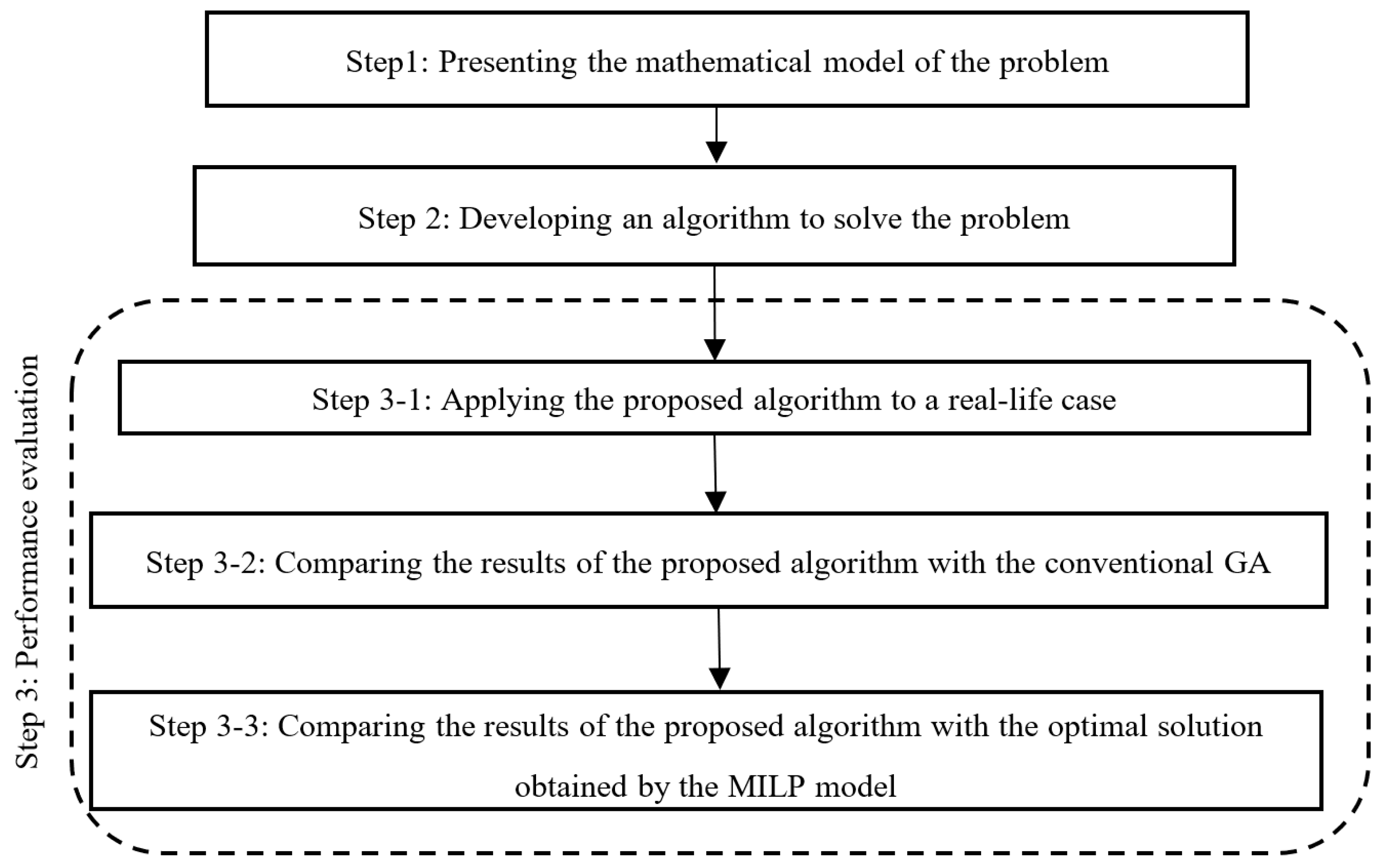
Figure 1 illustrates the research steps that are taken to address the presented questions.
The remainder of the paper is organized as follows. Section 2 gives a brief overview of the research background. Section 3 focuses on explaining the problem and presenting the mathematical model. The proposed algorithm is elaborated in Section 4. Numerical experiments are presented in Section 5. Finally, conclusions and suggestions for further studies are discussed in Section 6.
2. Literature Review
To date, different studies have been conducted on the scheduling problem in the supply chain context. Most of the existing studies integrated the production and scheduling problems. A review of the most relevant studies is provided below.
Averbakh [5] investigated the online scheduling in a supply chain network consisting of a factory and some customers aiming to minimize the load of orders. Four heuristic algorithms were proposed to solve the problem and competitive analysis was performed to study their worst-case performance. Rostamian Delavar, Hajiaghaei-Keshteli [6] presented a genetic algorithm to integrate production scheduling and air transportation. Two genetic algorithms for solving the problem were proposed after presenting a mathematical model. In another study, Scholz-Reiter, Frazzon [7] focused on the production and transportation in a general supply chain. The authors developed a mathematical model to cope with the problem. Kabra, Shaik [8] used mathematical programming to solve the scheduling problem in a pharmaceutical supply chain, considering multi-stage, multi-product, and multi-period environments. The authors extend a previous study by adding some limitations such as sequence-dependent changes, multiple delivery times, expiration date and defective products, and cost of late deliveries. Ullrich [9] integrated machine scheduling and vehicle routing considering time windows in a supply chain and proposed a genetic algorithm to solve the problem. Sawik [10] analyzed the relationship between scheduling and selecting the suppliers in case of disruption risks and presented a mixed-integer programming model for the problem. Han, Zhang [11] studied the scheduling of an online supply chain considering several customers and vehicles with limited capacity. The authors also minimized the total operation time and delivery cost in scheduling the online supply chain in the cases of single and parallel machines in a transportation system with one customer. Pei, Pardalos [12] solved the production and transportation scheduling problem in a two-stage supply chain in which the processing time is a linear function of its starting time. They considered two special cases and proposed two optimal algorithms to solve the problem. Beheshtinia, Ghasemi [13] used a modified version of the RGGA to solve the supply chain scheduling problem while considering a multi-site production system. Frazzon, Albrecht [14] presented a hybrid approach by combining mixed-integer linear programming, discrete event simulation, and a genetic algorithm to solve an integrated production and scheduling problem. Borumand and Beheshtinia [15] presented a new hybrid algorithm by mixing the genetic algorithm and an MCDM method for solving the integrated production and transportation supply chain problem. Beheshtinia and Ghasemi [16] presented a metaheuristic algorithm called multiple league championship algorithm (MLCA), including two operators of practice and tournaments to address the supply chain scheduling problem. Najian and Beheshtinia [17] presented an improved genetic algorithm called RGGA to solve the same problem while simultaneously cross-dock and vehicle routing methods were applied for transportation. Sarvestani, Zadeh [18] presented a heuristic algorithm to tackle the scheduling problem in a supply chain network considering several cases such as accepting the order, determining the delivery date, and selecting the supplier. Taheri and Beheshtinia [19] studied the integration of production and transportation scheduling in a two-stage supply chain to minimize total earliness and tardiness simultaneously. In this study, a time window due date for each order is considered. The authors developed a GA considering traveling chromosomes between various generations of GA to solve the problem. Gharaei and Jolai [20] discussed the integration of production and scheduling problems in a supply chain composed of a manufacturer and its customers. To cope with the problem, the authors proposed two heuristic algorithms based on the decomposition approach. The considered objective functions were to minimize total tardiness and transportation cost. Ying, Pourhejazy [21] discussed the distributed assembly permutation flow-shop scheduling problem with flexible assembly and sequence-independent setup times. The authors presented an original mixed-integer linear programming model and proposed a heuristic and an Iterated Greedy Algorithm (IGA) to cope with the problem’s complexity.
Beheshtinia, Salmabadi [22] considered a two-layer transportation system in a three-echelon supply chain. The authors integrated production and routing problems and proposed a mathematical model to minimize production costs, transportation, inventory holding, and expired drugs treatment. Furthermore, they proposed a possibilistic model and a robust possibilistic model corresponding to the initial model to consider the uncertain nature of the problem. Bank, Mahdavi Mazdeh [23] proposed two mixed-integer linear programming models to optimize four objective functions in an integrated production–distribution system considering lot-sizing decisions. The considered objective functions were total sequence-dependent setup costs, holding costs, delivery costs, and delay penalties. Furthermore, a hybrid genetic algorithm is proposed to solve the problem in large-scale problems. Purnomo, Anugerah [24] discussed a collaborative supply chain in the furniture industry and tried to minimize material, processing, transportation, and holding costs. They developed a mathematical model and proposed a genetic algorithm to solve the problem. Pourhejazy, Cheng [25] integrated the production scheduling and distributed manufacturing operations. They addressed the distributed two-stage assembly flow-shop with sequence-dependent setup times. To tackle the problem, they proposed a mixed-integer linear programming model and an iterated greedy algorithm to minimize the makespan. Aminipour, Bahroun [26] studied the cyclic production scheduling problem in a two-stage closed-loop supply chain while assuming that material shortage is not allowed. The considered optimization objective was to minimize the sum of holding and setup costs. After proposing the mixed-integer linear mathematical model of the problem, a heuristic algorithm is proposed to solve large-scale problems. Moghimi and Beheshtinia [27] discussed the integration of production and scheduling problems in a supply chain considering the multi-site manufacturing system. They considered two objective functions of minimizing total tardiness and environmental pollution and proposed a genetic algorithm with multiple parallel populations two solve the problem. Wang [28] investigated the integrated production and transportation scheduling problem in a three-stage supply chain composed of a set of heterogeneous suppliers at the first stage, a set of capacitated manufacturers at the second stage, and a set of retailers at the third stage. The authors proposed a nonlinear mathematical model and a hybrid particle swarm optimization (PSO) algorithm to tackle the problem. The considered objective functions were to minimize the total shipping and penalty costs. Rahman et al. [29] discussed the integration of production and transportation scheduling problems in a two-stage supply chain composed of a manufacturer in the first stage and a set of customers in the second stage. They considered sequence-dependent setup times and permutation flow shop environment. After presenting a nonlinear mathematical model of the problem, the authors proposed three metaheuristic algorithms, namely Differential Evolution (DE), Moth Flame Optimization (MFO), and Lévy–Flight Moth Flame Optimization (LFMFO), to optimize the total cost of tardiness and batch delivery.
The literature review shows that the existing studies in terms of integration level can be divided into three groups: (1) integration of suppliers and manufacturers, (2) integration of manufacturers and distributors, and (3) integration of suppliers, manufacturers, and distributors, which is known as a hybrid. Moreover, the studies are also classified into two groups in terms of time consideration. Some studies considered the time a continuous parameter, while others considered it several discrete periods.
In terms of the objective function, the existing studies are either single-objective or multi-objective. Although many studies in the literature claimed to be multi-objective, most of the studies converted all the objective functions into cost and merged them. Therefore, the effect of the proposed solutions on each objective function has been rarely investigated.
As for the solution method, a mathematical model was proposed in most studies as the primary solution method. However, most of the studies have resorted to a heuristic algorithm, mainly GA, to cope with the complexity of the problem. The literature review also shows that most previous studies considered the suppliers or manufacturers as a single-machine environment. Some other production environments, such as assembly flow-shop, parallel machines, flexible flow-shop, and flexible job-shop, received less or no attention. A summary of the reviewed studies is provided in Table 1. To complement the existing literature on SCCP, in the current research, each production unit is assumed to have an FJS environment, one of the most general production environments, and other environments are reduced versions of FJS. The current research also differs from the previous studies by addressing the SCCP while integrating transportation and production scheduling and considering multiple objectives, namely minimizing the total orders’ delivery time, transportation and production costs, pollution levels, and maximizing the quality of completed orders.
The contribution of this study can be summarized as follows:
- Investigating the scheduling in the supply chain by considering a distributed manufacturing system and multiple objectives;
- Considering each manufacturer as an FJS environment;
- Presenting a mathematical model for the problem;
- Introducing an efficient algorithm by combining GA and TOPKOR method (GA-TOPKOR).
3. Definition of the Problem
The problem explanation, including its assumptions, parameters, and the mathematical model of the problem, is presented in this section.
3.1. Problem Specifications
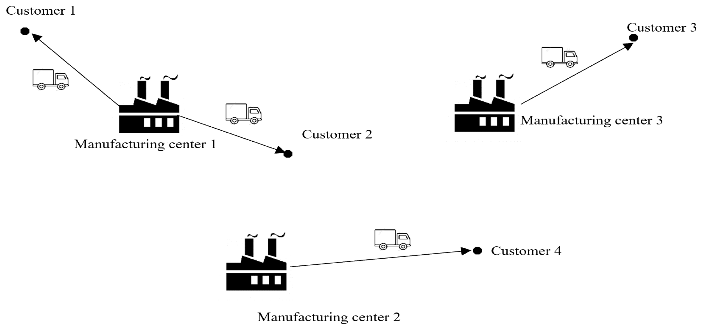
The present study assumes that a factory including several separated manufacturing units should process orders and deliver them to customers. Each manufacturing unit has a flexible job-shop (FJS) environment. It is assumed that a set of n orders O = {O1, O2, …, On} should be processed by a set of u manufacturing units U = {MU1, MU2, …, MUu} which are scattered in different regions. Every order should be processed by just one single manufacturing unit. Each order is composed of a set of operations in which the number of the operations of the ith order is shown as . As the technology of each machine may be different in each manufacturing unit, it is assumed that the number of operations for each order in some manufacturing units may be different. In other words, the orders’ process route may be different (i.e., this is a generalized form of the case in which the production process does not depend on the manufacturing unit and is the same in all units). Each manufacturing unit has a set of production machines = {, …, , …, }. After assigning an order to one manufacturing unit, the order’s operations can be processed on a set of allowed machines. Orders should be delivered to the related customer after they are completed. Thus, one transportation time and one transportation cost should be considered for each order. Figure 2 shows a schematic view of the considered supply chain.
Other assumptions are as follows:
- The processing time and production cost of each operation depend upon both the selected manufacturing unit and the selected machine;
- The transportation time, transportation cost, level of pollution, and quality of completed orders are predetermined, and they may be dissimilar in different manufacturing units;
- The delivery time of an order equals the completion time of its last operation and the time of transportation from the assigned manufacturing unit to the related customer;
- All operations and all machines in all manufacturing units are available at the time zero;
- Each machine in every manufacturing unit can only process one operation at a specific moment;
- Each order should be assigned to only one manufacturing unit. If an order is assigned to a manufacturing unit, all of its operations should be processed inside that unit;
- Disruptions are not allowed. In other words, each operation should be processed without interruption once its process starts;
- Some manufacturing units may not be able to process some orders. Moreover, some machines may not be able to process some operations.
It is worth mentioning that some parameters like operation cost can be altered. In this study, operation cost is related to the machine and manufacturing unit that each operation is assigned. This means that changing the assigned manufacturing unit and machine of each operation changes its operation cost.
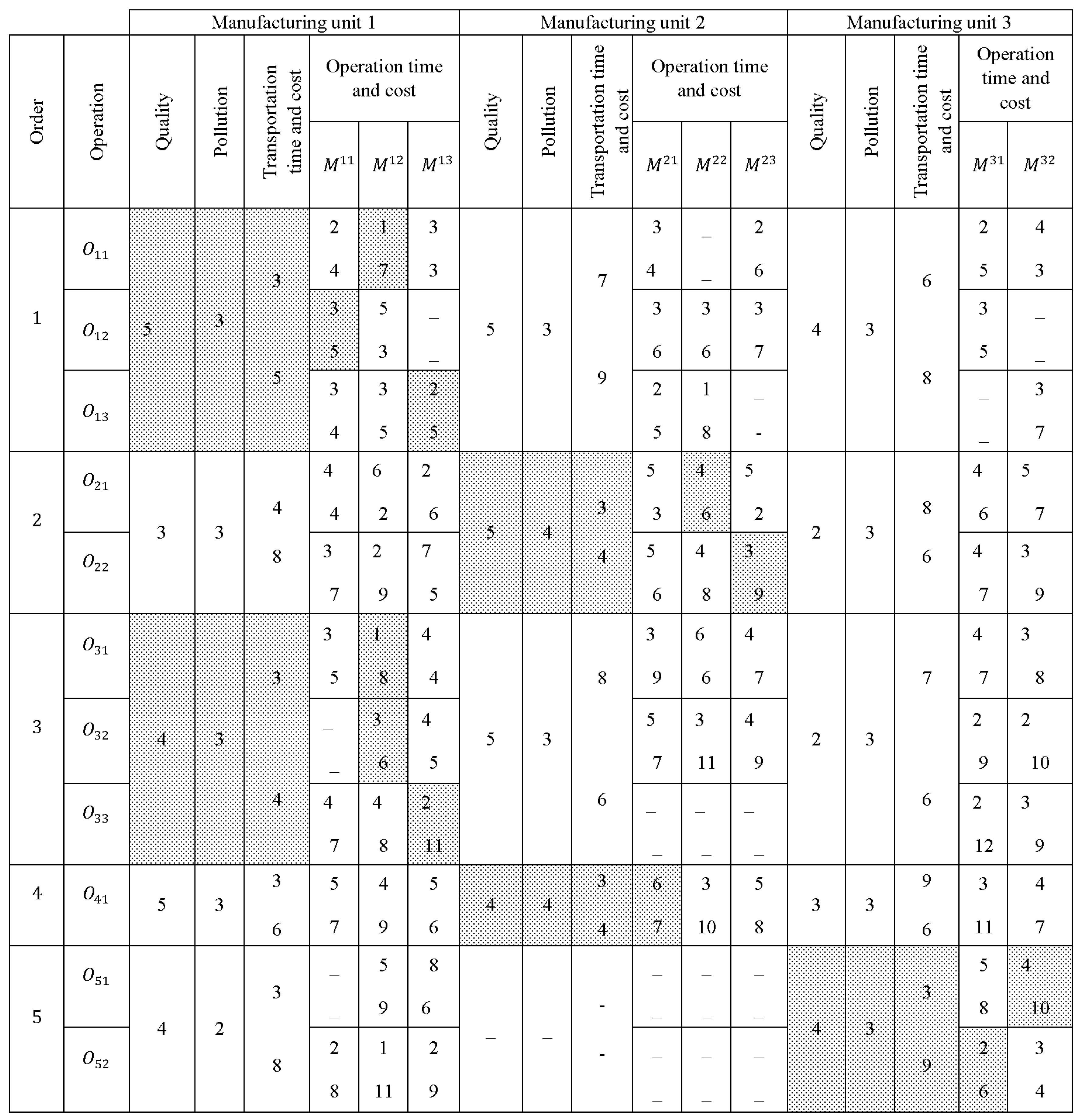
Figure 3 shows an example with three manufacturing units and five orders in which orders 1 to 5 have 3, 2, 3, 1, and 2 operations, respectively. Manufacturing units 1 to 3 have 3, 3, and 2 machines, respectively. In some cells, two numbers are shown, the top number displays time, and the bottom one is the cost. The data (i.e., transportation cost and time, quality, and level of pollution) related to each order when it is assigned to a manufacturing unit are also given in the figure. Allocating some orders to some manufacturing units and some operations to some machines are not allowed, and these cases are shown as “-” in Figure 3. In addition, one feasible solution is highlighted in which orders 1 to 5 were assigned to 1, 2, 1, 2, and 3, respectively. Further, , and are assigned to , and , respectively. Accordingly, to obtain the final solution, the priority of processing the orders assigned to a machine should be determined. For instance, two operations of and were assigned to and their processing should be prioritized.
3.2. Mathematical Model
In this section, the mathematical formulation of the problem is presented. The presented model is an extension of the model proposed by Ziaee [30]. The original model only addresses production scheduling and does not consider transportation scheduling. However, in the current study, the integration of production and transportation problems is investigated. Consequently, some parameters, variables, and constraints related to transportation time and cost are added to the model. Additionally, multiple objectives are considered: minimizing the total orders’ delivery time, transportation and production costs, pollution levels, and maximizing the quality of completed orders.
The parameters of the model are as follows:
Sets:
I: Set of orders
S: Set of manufacturing units
J: Set of operations
K: Set of machines
Indices:
i: Order index (i = 1, …, n)
s: Manufacturing unit index (s = 1, …, u)
j: Operations index (j = 1, …, noi)
k: Machine index (k = 1, …, )
l: Sequence index of assigned operations to machine k (1, …, dsk)
Parameters:
: Maximum number of operations that can be assigned to machine k of manufacturing unit s
n: Number of orders
u: Number of manufacturing units
: Number of machines in manufacturing unit s
: Number of operations of order i
Aijsk: A zero-one parameter in which Askij equals 1, if Oik can be processed by the machine k of manufacturing unit s; otherwise, it equals 0
Pijsk: Processing time of operation Oij on machine k of manufacturing unit s
TTimeis: Transportation time of order i if it is assigned to manufacturing unit s
TCostis: Transportation cost of order i if it is assigned to manufacturing unit s
OCostijsk: Operation cost of Oij if it is assigned to machine k of manufacturing unit s
Qis: Quality of completed orders i if it is assigned to manufacturing unit s
Polis: Produced pollution if order i is assigned to manufacturing unit s
M: A sufficiently large number
Decision variables:
RPij: Real processing time of operation Oij after choosing a machine
RTCosti: Real transportation cost of order i after being assigned to a manufacturing unit
RTTimei: Real transportation time of order i after being assigned to a manufacturing unit
ROCostij: Real operation cost of operation Oij after being assigned to a machine
Deli: Delivery time of order i
Yijsk: Equals 1, if machine k of manufacturing unit s is selected to process Oij; otherwise, Yijsk = 0
Xijskl: Equals 1, if Oij is processed on machine k of manufacturing unit s with the priority l; otherwise, Xijskl = 0
MUis: Equals 1, if order i is assigned to manufacturing unit s; otherwise, MUjs = 0
Tij: Start time of processing Oij
TMskl: Start of working time for machine k of manufacturing unit s in priority l
Considering the above notations, the problem can be formulated as the mixed-integer linear programming (MILP) model presented below.
| (1a) | ||
| (1b) | ||
| (1c) | ||
| (1d) | ||
| (1e) | ||
| Subject to: | ||
| = 1 | i | (2) |
| × TTimeis = RTTimei | i | (3) |
| × TCostis = RTCosti | i | (4) |
| = 1 | i,j | (5) |
| Yijsk ≤ Askij*MUis | i,j,s,k | (6) |
| × OCostijsk = ROCostij | i,j | (7) |
| × Pijsk = RPij | i,j | (8) |
| = 1 | s,k,l | (9) |
| = 1 | i,j | (10) |
| i,j,s,k,l = 1, …, | (11) | |
| = | i,j,s,k | (12) |
| TMskl+RPij ≤ TMsk(l+1) + M(1 − Xijskl) | i,j,s,k,l = 1, …, −1 | (13) |
| TMskl≤Tij + (1 − Xijskl) × M | i,j,s,k,l | (14a) |
| TMskl + (1 − Xijskl) × M ≥ Tij | i,j,s,k,l | (14b) |
| Tij + RPij ≤ Ti(j+1) | i,j = 1, …, −1 | (15) |
| Deli ≥ + + | i | (16) |
| Deli,RTCosti, RTTimei ≥ 0 | i | (17) |
| ROCostij, RPij,Tij ≥ 0 | i,j | |
| MUis{0,1} | i,s | |
| TMskl ≥ 0 | k,l | |
| Yijsk{0,1} | i,j,s,k | |
| Xijskl{0,1} | i,j,s,k,l | |
Equation (1a–e) demonstrate the objective functions of the problem that are minimizing total delivery time of orders, total transportation costs, total operation costs, total created pollutions, and maximizing the quality of the total orders, respectively. Constraint set (2) indicates that each order should be assigned to one manufacturing unit. The real transportation time and cost of each order are determined by constraint sets (3) and (4), respectively. Constraint set (5) ensures each operation is only assigned to one machine. Constraint set (6) prevents assigning operations to unacceptable machines. Constraint sets (7) and (8) determine the real operation cost and real processing time of each operation, respectively. Constraint set (9) prevents assigning an identical priority to different operations. Constraint set (10) indicates that each operation should be assigned to one machine and one priority of this machine. Constraint set (11) prevents assigning zero values between the priorities of a machine. Constraint set (12) guarantees that if an operation is not allocated to a machine, it cannot be assigned to any priority of that machine. Constraint (13) indicates that two operations cannot be processed by the same machine, simultaneously. Constraint sets (14a) and (14b) links between the start time of each operation and the availability of the machine to start processing it. The start times of Oij and Oi(j+1) are linked by Constraint set (15). The delivery time of each order to its related customer is calculated by Constraint set (16). The type and the sign of variables are defined by the Constraint set (17).
4. The Proposed Solution Algorithm
To solve the problem, a combination of TOPKOR (i.e., an MCDM technique) and the genetic algorithm, called GA-TOPKOR, is proposed. An overview of the GA and TOPKOR method is provided in Section 4.1 and Section 4.2, respectively. Then, the proposed algorithm is presented in Section 4.3.
4.1. Genetic Algorithm
The genetic algorithm (GA) is a widely used method for solving complex optimization problems known as NP-hard problems [31]. The GA is inspired by the evolution mechanisms of nature. In this algorithm, every answer is displayed as a chromosome [32]. As the first step to solve a problem using GA, some chromosomes are generated randomly. Then, new chromosomes are produced by crossover and mutation operators. Subsequently, some chromosomes are transferred to the next generation by the selection operator. This process is reiterated until the algorithm termination criterion is satisfied.
4.2. TOPKOR Method
The TOPKOR method, proposed by Sedady and Beheshtinia [33], is an MCDM method that rates the alternatives based on a set of criteria. In the TOPKOR method, an alternative gets a good rank if it has low values in two parameters of total difference with a positive ideal solution, the maximum difference with the positive ideal solution in each criterion, and a high value in the parameters of total difference with the negative ideal solution. The steps of the TOPKOR method, when there are Nc criteria and Nm alternatives, are as follows.
Step 1: Present the scores of alternatives in each criterion as decision matrix and the vector of criteria weights as input (xac is the score of alternative a in criterion c and wc is the weight of criterion). A sample decision matrix is presented in Equation (18).
Step 2: Normalize the decision matrix arrays (nac is the normalized score of alternative a in criterion c) as presented in Equation (19).
Step 3: Calculate the weighted normalized matrix (vac is the weighted normalized score of alternative a in criterion c) using Equation (20).
Step 4: For criterion j obtain the Positive Ideal Solution (PIS) and Negative Ideal Solution (NIS) as presented in Equation (21).
In which B represents the set positive criteria such as benefit, and C represents the set of negative criteria such a cost.
Step 5: Obtain the total distances of each alternative from PIS and NIS using Equation (22).
where is the total distance of alternative a from PIS (utility index) and is the total distance of alternative a from NIS (inutility index).
Step 6: Calculate the maximum distance between each alternative and PIS in each criterion (Regret index) using Equation (23).
Step 7: Obtain VIKOR index (Qa) using Equation (24).
where , , , and v is a parameter of the TOPKOR method whose value is between 0 and 1. It indicates the relative weight of the normalized utility index against the normalized regret index. In this research, to obtain identical weights to both indices, v is considered as 0.5.
Step 8: Calculate the closeness coefficient index for the alternative Aa, indicated by CCa, using Equation (25). The alternative with a higher value for CCa is more desirable.
4.3. GA-TOPKOR Algorithm
The structure of GA-TOPKOR is the same as that of a conventional genetic algorithm but with a significant difference in the selection operator when transferring solutions from one generation to another. To transfer the chromosomes to the next generation in the selection operator of GA, the chromosomes should be compared with each other. Considering a problem with two objective functions, in each comparison, one chromosome may obtain a better value in an objective function and a worse value in the other one. In this case, choosing the better chromosome may be challenging, and it is more complicated when the number of objective functions increases.
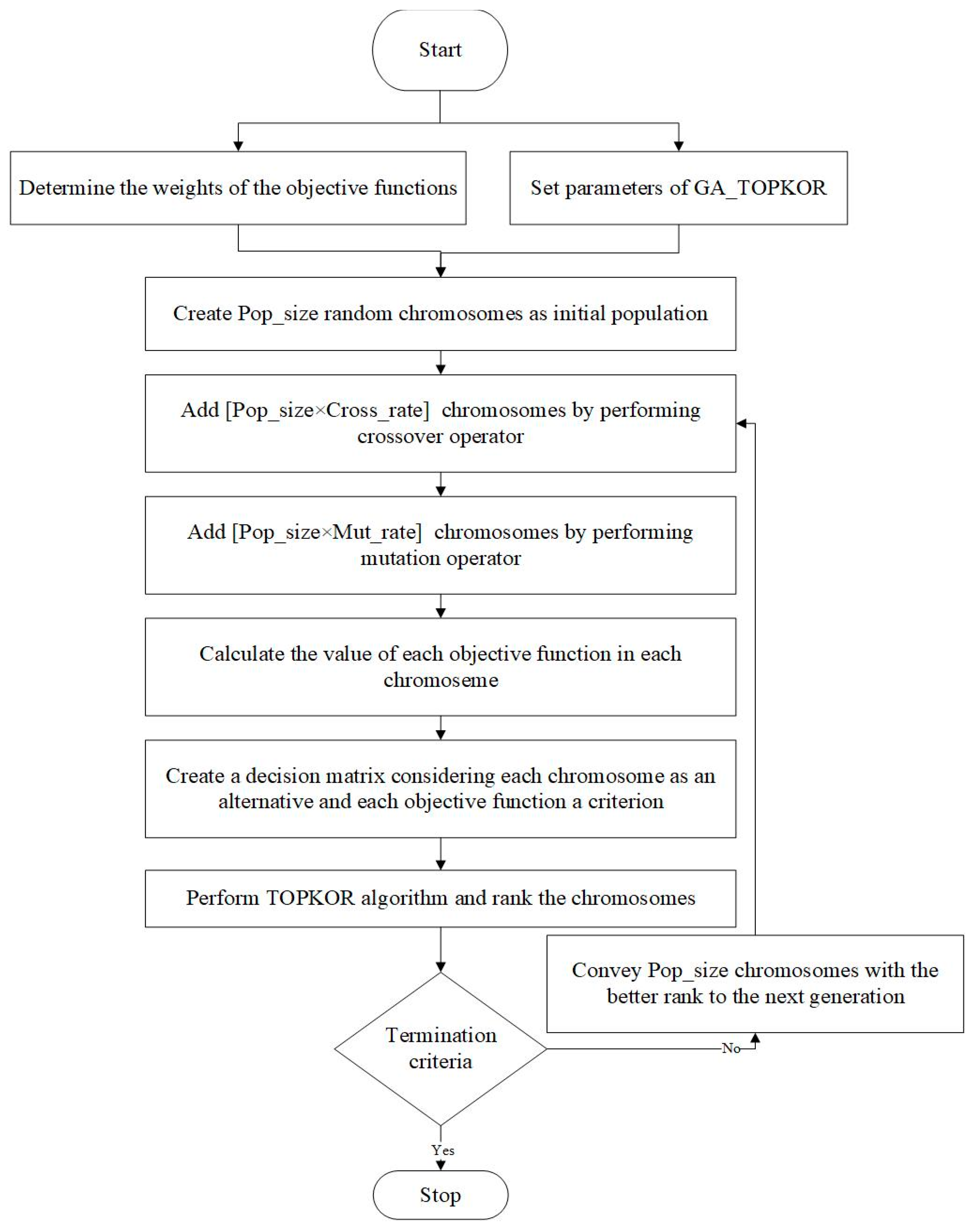
The GA-TOPKOR uses the TOPKOR method to select the superior chromosomes and transfer them from one generation to the next. In this regard, chromosomes and objective functions are considered as alternatives and criteria, respectively. The main septs of GA-TOPKOR are presented below and also depicted in Figure 4 for better clarification.
Step 0: Determine the weights of the objective functions and set parameters of GA-TOPKOR.
Step 1: Produce random chromosomes as the initial population, called Pop_size. Pop_size indicates population size and it is one of the GA-TOPKOR parameters.
Step 2: Select two random chromosomes and perform a crossover operator. Repeat this step [Pop_size × Cross_rate] times and add the new chromosomes to the current population. Cross_rate indicates crossover rate and it is one of the GA-TOPKOR parameters.
Step 3: Select a random chromosome and perform the mutation operator. Repeat this step [Pop_size × Mut_rate] times and add the new chromosomes to the current population. Mut_rate indicates mutation rate and it is one of the GA-TOPKOR parameters.
Step 4: Consider chromosomes as alternatives and objective functions as criteria and perform the TOPKOR method to rank the chromosomes. In this case, the closeness coefficient index related to each chromosome is considered as its fitness function.
Step 5: If the best fitness value of chromosomes is not changed after a certain number of successive generations, represented as Ter_Num in the proposed algorithm, terminate the algorithm. It should be noted that Ter_Num is a parameter of the algorithm and should be determined in the parameter setting of the algorithm.
Step 6: Transfer Pop_size chromosome with better rank to the next generation and go to Step 2.
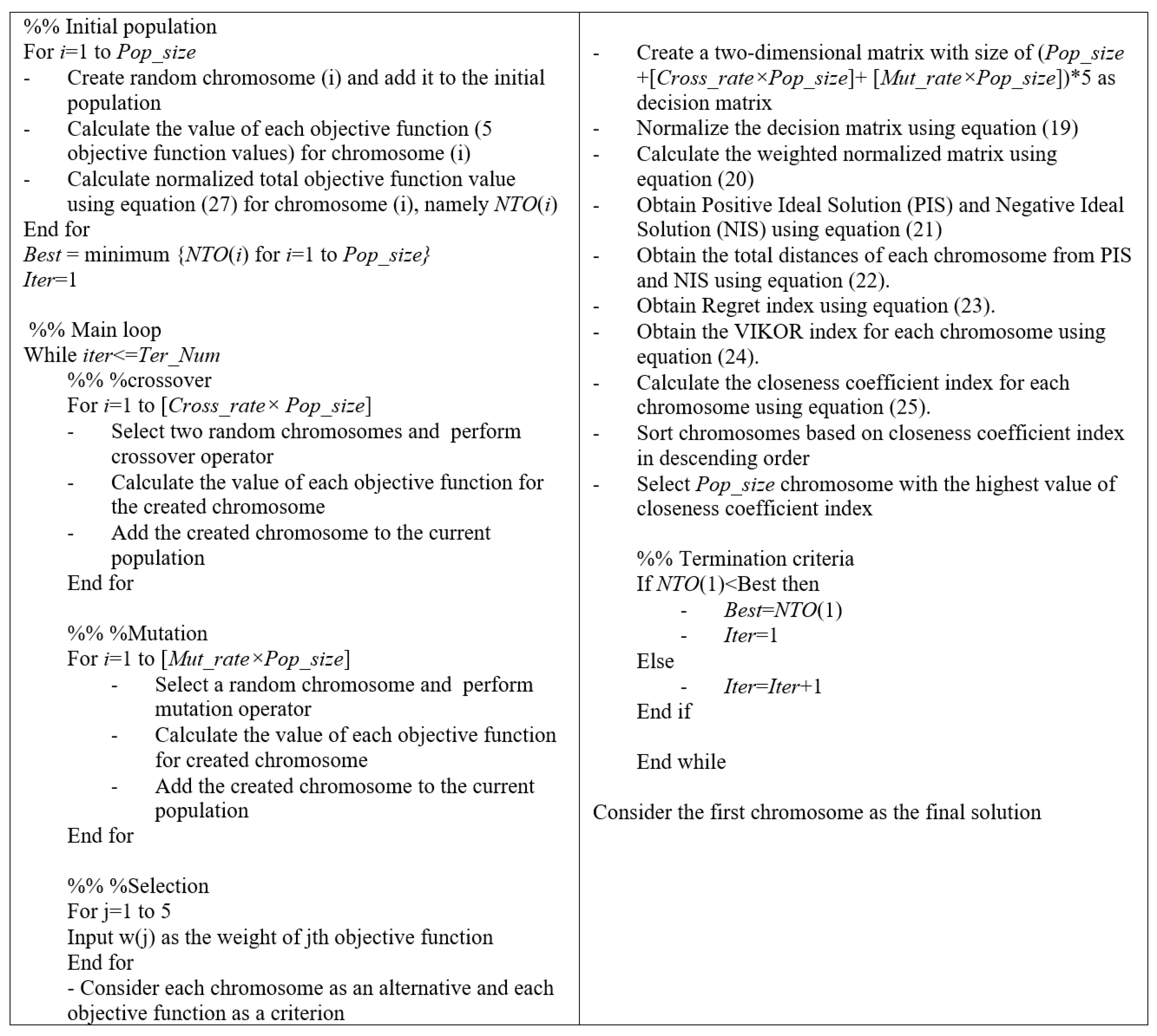
To better clarify the solution procedure, the pseudocode of the GA-TOPKOR is presented in Figure 5. In this pseudocode, Iter is a counter that shows the number of successive generations that the best fitness value of chromosomes has not been changed.
4.3.1. Solution Representation
Each solution should be represented in the form of chromosomes. Therefore, chromosomes should include some information such as the manufacturing unit assigned to each order, the machine assigned to each operation, and the sequence of orders assigned to the same machine. Three strings were used to encode each solution to one chromosome. These strings are as long as the total number of orders’ operations. Each array (gene) of the string corresponds to one operation. The first string shows the assigned manufacturing unit to process the related operation (order). Since all the operations related to one order should be assigned to one manufacturing unit to create random numbers for the first string, just the first operation of each order is given the random number and this number is replicated for other operations of that order. The numbers within the second string show the machine number in the manufacturing unit related to that operation. The string numbers are randomly selected considering the unit assigned to the mentioned order in the first string and among the allowed machines. The third array numbers include a real number between 0 to 1 and are used for prioritizing the operations assigned to each machine.
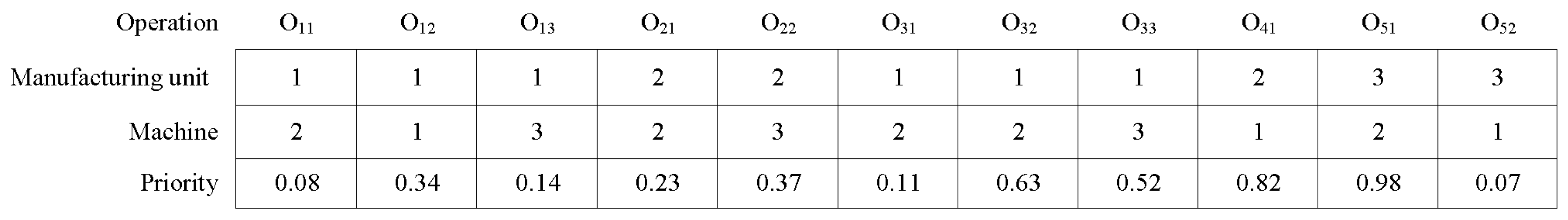
Accordingly, if in the second string, two operations are assigned to the same manufacturing unit and machine, the order with a lower decimal number will be given a higher priority. To better illustrate the proposed solution representation, a feasible chromosome for the example presented in Figure 3, is shown in Figure 6.
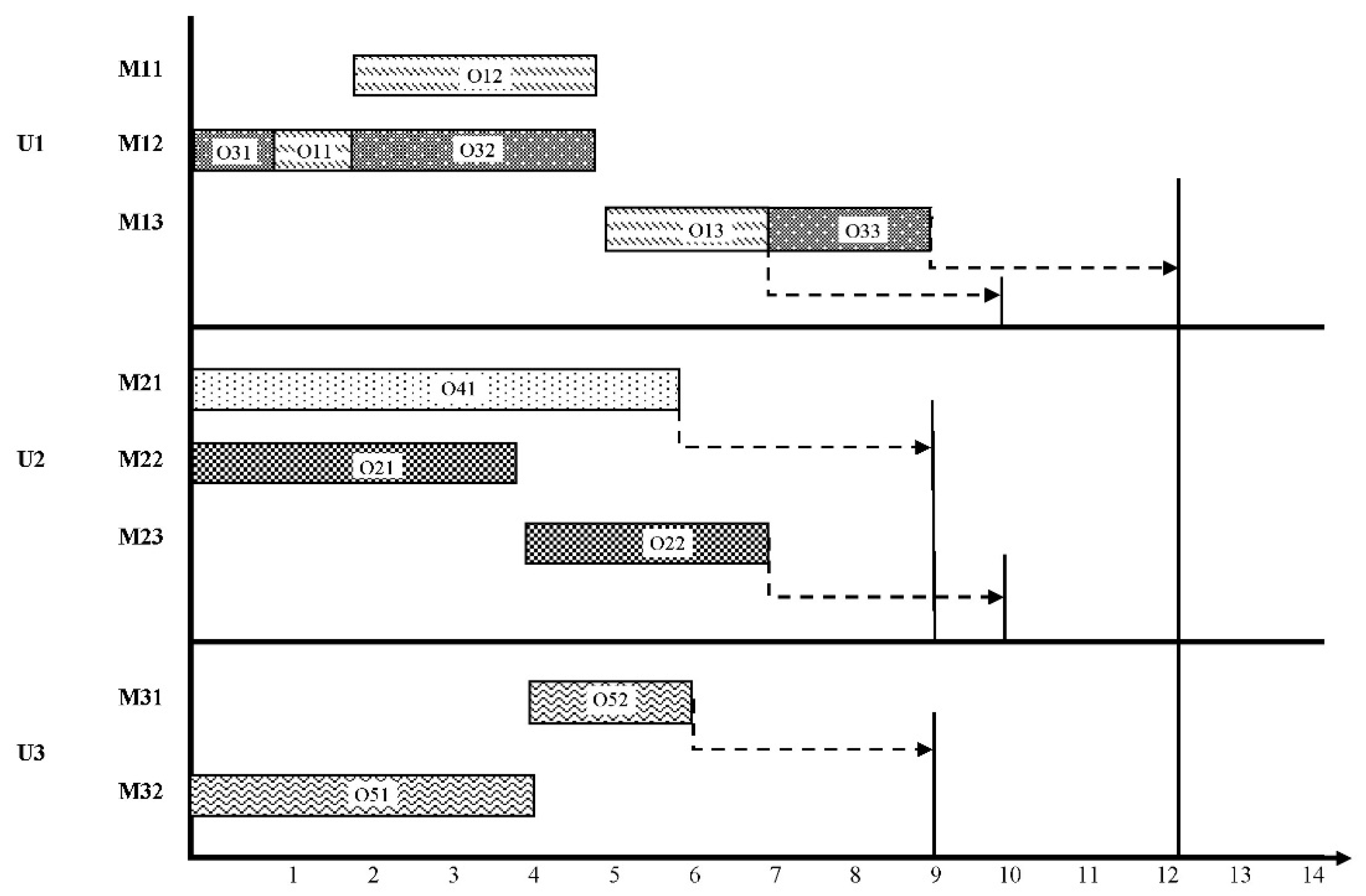
After allocating the orders to manufacturing units, operations to machines, and determining operations sequences for each machine, the solutions can be scheduled to calculate each objective function. Figure 7 displays the Gantt chart of the solution corresponding to the presented chromosome. Table 2 shows all the objective functions related to this solution.
4.3.2. Crossover and Mutation Operators
In this study, two crossover operators, namely double-cut point and single-cut point operators, were used. Furthermore, the swap operator was used for the mutation operation. To find more about the crossover and mutation operators mechanism, interested readers may refer to [34]. Suppose operations related to a certain order are assigned to different manufacturing units as a result of a crossover operator in a child chromosome. In that case, a modification procedure will be initiated in which all the operations will be assigned to the manufacturing unit related to the order’s first operation. If the operations assigned to a machine are not feasible in the second string, the machine number will randomly change to a feasible machine using a modification procedure.
5. Numerical Experiments
In this section, GA-TOPKOR is compared with a classical genetic algorithm named CGA. The structure of the CGA is the same as GA-TOPKOR, but no MCDM method is used for selecting and transferring the solutions. To test the performance of the GA-TOPKOR, a set of generated problems and a real case taken from a sofa manufacturer are solved. The proposed GA-TOPKOR is also compared with the optimal solutions obtained by a commercial solver for small-size problems. The algorithm is coded in MATLAB and run on a computer with a 1.90 GHz CPU and 4 GB RAM.
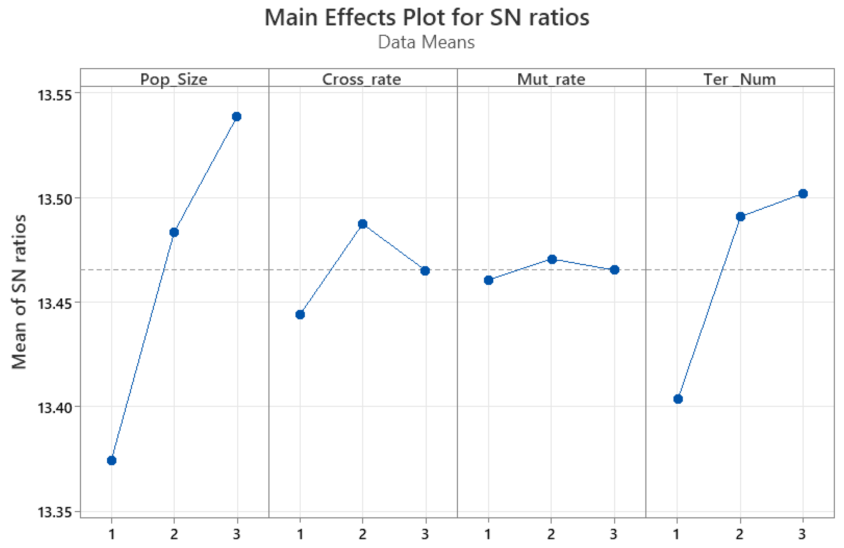
To determine the best value of the algorithm’s parameters Taguchi method is employed. More details about the Taguchi method can be found in [35]. The main parameters of the GA-TOPKOR are Pop_Size, Cross_rate, Mut_rate, and Ter _Num. Table 3 shows the considered levels for each parameter to perform the Taguchi method. Figure 8 indicates that based on the signal-to-noise (SN) ratio, the value of 100 for Pop_Size, 0.7 for Cross_rate, 0.3 for Mut_rate = 0.3, and 10 for Ter_Num result to better performance.
5.1. Case Study
In order to evaluate the performance of GA-TOPKOR, it was examined by a real data set collected from a sofa manufacturer. The result of the GA-TOPKOR was then compared with that obtained from the current situation. The manufacturer’s production and distribution system information were collected for one month (from 8 October 2018 to 9 November 2018).
The furniture company has three manufacturing units in different regions. There are 19 related orders which should be assigned to these three manufacturing units. Each order belongs to a specific customer. Each of these orders needs some operations to be completed, such as cutting, forming, assembling the wooden skeleton, polishing, painting, putting upholstery, assembling mattresses, and packaging. The orders are of six types of furniture, namely wooden, modern, corner, chair, L-shape, and three-seater with different designs and different production routes. Additionally, the weight of each objective function was determined based on the opinion of experts and the analytic hierarchy process (AHP) technique. The weights obtained for the objective functions of the sum of delivery times, transportation costs, production costs, pollution level, and quality of completed orders were 0.44, 0.27, 0.02, 0.09, and 0.18, respectively.
Comparing the results obtained from GA-TOPKOR with those from the current situation suggests a 42% improvement in delivery times, 38% in total transportation cost, 25% in production costs, 3% in quality of completed orders, and the level of pollution remained unchanged (Table 4).
5.2. Comparison of GA-TOPKOR and CGA
In this section, GA-TOPKOR is compared to CGA. The structure of CGA is the same as that of GA-TOPKOR, with the only difference being that TOPKOR is not used in the selection operator. To find which chromosome is better in CGA, Equation (26) is used as the fitness function of the jth chromosome in each generation.
where , , and represent the weight of the ith objective function, the value of the ith objective function in chromosome j, the maximum value of the ith objective function, and the minimum value of the ith objective function for the chromosomes of the current generation, respectively. The first and second terms of fitness value presented in Equation (26) are related to minimizing the four first objective functions and maximizing the fifth objective function (the quality of completed orders), respectively.
After obtaining the final solution of both algorithms, the index presented in Equation (27) is used to compare the quality of the solutions.
indicates the ideal value for the ith objective function. The ideal value for each objective function was obtained by applying the genetic algorithm and placing 1 for the weight of that objective function and 0 for the weight of others and using a relatively large population size (10,000 in this study). The solution with a lower value for normalized total objective function has better quality.
To evaluate the performance of the GA-TOPKOR, a set of test problems have been generated and solved by both the GA-TOPKOR and CGA. Four parameters were considered to generate the test problems, including the number of orders, operations for each order, manufacturing units, and manufacturing machines. As shown in Table 5, different levels were determined for each parameter. In Table 2, U [a,b] means that one integer value in the range of a to b is randomly selected for the parameter.
Using the information given in Table 5, 24 (3 × 2 × 2 × 2) random problems were generated as presented in Table 6. For other parameters of the problem, only one level was considered. The orders’ process times and the costs and times of transportation were randomly selected from a uniform distribution of U[20,40] Parameters of quality of completed orders and pollution are selected randomly from a uniform distribution of U[1,5] with regard to the Likert spectrum. In addition, the weights of objective functions are considered equal to the same weights obtained from the case study.
Considering the random nature of GA, the results may be different in each performance. Therefore, each test problem was solved 30 times by GA-TOPKOR and CGA, and the following hypothesis was tested. Since the number of samples for each test problem is 30 (for each test problem, the sample size is 60 = 30 samples from GA + 30 samples from GA-TOPKOR), the T-student distribution with degree of freedom 58 (i.e., 30 + 30 − 2) is used for statistical hypothesis testing.
Hypothesis 0 (H0).
The average of normalized total objective function from GA-TOPKOR is equal to this average for CGA.
Hypothesis 1 (H1).
The average of normalized total objective function from GA-TOPKOR is smaller than this average for CGA.
The results of the comparison between GA-TOPKOR and CGA are presented in Table 7. The results given in Table 4 show that P-value is less than 0.05 for all the problems solved except for one case. Thus, H0 is rejected, and H1 is accepted. This means that GA-TOPKOR outperforms CGA.
The comparison results also revealed that using TOPKOR in the genetic algorithm’s selection operator improves the algorithm’s results in this multi-objective optimization problem.
5.3. Comparison with the Optimum Solution
To evaluate the performance of GA-TOPKOR further, the results obtained from this algorithm for the small-size problems were compared with the optimal solution obtained from the mathematical model. The values considered for the parameters of the small-size test problems are shown in Table 8. Moreover, the obtained results by solving these test problems by GA-TOPKOR and the optimum solution are presented in Table 8.
The optimal solutions were obtained using GAMS software. The comparison results indicated that GA-TOPKOR found the optimal solution for most solved instances in much less CPU time than the GAMS software. It is also worth noting that the difference was insignificant for cases in which GA-TOPKOR could not find the optimal solution.
5.4. Discussion
This section provides a discussion on the algorithm features and the implications of the conducted study.
5.4.1. Algorithm Features
CGA and GA-TOPKOR have similar structures, but their selection operators are different. CGA gives a higher chance of being selected to chromosomes with a low normalized distance from a PIS in each generation. However, GA-TOPKOR considers three parameters of the total distance from PIS (), maximum distance from PIS in each criterion () and total relative distance from NIS (). GA-TOPKOR gives a higher chance of being selected to chromosomes with low values for (), and , and high value for . In other words, a chromosome may not have a short total distance to the PIS, but it has a low value for regret index or a long distance to the negative ideal solution.
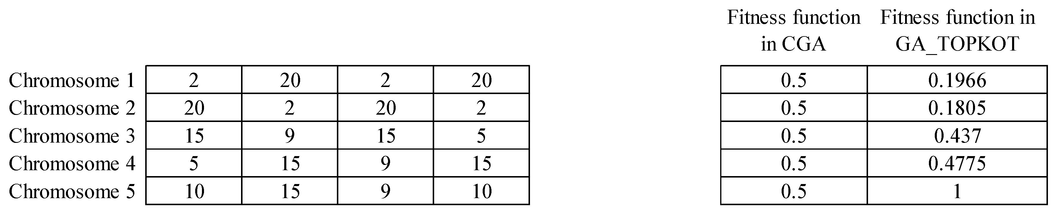
For example, consider a problem with four minimization objective functions in which the weights of all objective functions are equal to 0.25. Indeed, the fitness function of CGA calculates the distance of each chromosome from NIS. If there are five chromosomes, as shown in Figure 9, then the fitness values of the chromosomes are the same in CGA. In this particular case, a random selection operator has the same performance as the selection operator of CGA. While in GA_TOPKOR, the chromosomes have different fitness values. The reason is that GA-TOPKOR considers three parameters of the maximum distance of each chromosome from PIS in each criterion, its total distance from PIS, and its total distance from NIS, while CGA considers only the distance of each chromosome from NIS.
5.4.2. Implications of the Study
This research may serve researchers active in the supply chain optimization field by proving knowledge on the importance of selection mechanisms when using population-based algorithms. This also provides insight into the usefulness of employing MCDM methods in intelligent algorithms when dealing with multiple objectives. In practice, managers often deal with multiple conflictive objectives when optimizing their supply chain network. This means that optimizing one objective may negatively affect other objectives. For instance, minimizing the delivery time can affect other criteria such as cost or quality. In this case, choosing the best solution might be challenging, and MCDM methods could assist the decision-makers. This study showed how MCDM methods could be combined with an optimization algorithm to improve the solution quality.
Considering the promising performance of the proposed algorithm in dealing with SCSP, it can aid decision-makers and supply chain managers to optimally design their supply chain networks while satisfying both economic and environmental concerns. Considering the possible opportunities for energy sustainability discussed in the recent literature (e.g., [36]), this study may also allow managers to get one step closer to the resource and energy-efficient supply chain concept.
This study also contributes to sustainable supply chains by considering two essential sustainability aspects (i.e., environmental and economic) as the main optimization objectives. The economic concerns are addressed by optimizing the total delivery time of order, transportation cost, and production cost. The environmental concerns are handled through optimizing the environmental pollution, and the quality of products contributes to the environmental aspect. The results of the computational student and the considered real case showed the effectiveness of the proposed algorithm in efficiently improving the economic and environmental aspects.
6. Conclusions and Future Research Directions
This study investigates the scheduling problem in a supply chain network consisting of a manufacturer with multiple sites scattered in different regions and its customers. Each production unit is assumed to have a Flexible Job-Shop environment. A new algorithm named GA-TOPKOR that uses TOPKOR as an MCDM technique in the selection operator of the genetic algorithm (GA) was proposed to solve the problem.
The performance of the GA-TOPKOR was compared with the conventional GA for large-scale problems and with the optimum solution for small-size problems. The results showed that including TOPKOR as an MCDM technique in the GA’s selection operator enhances the performance of the GA. The proposed algorithm was also applied to a real-life case study and significantly improved the process compared to the current situation. Overall, all the comparisons collectively showed that the proposed GA-TOPKOR is efficient in finding a good solution to the supply chain scheduling problem.
Despite the effort made to make the problem compatible with the real-world need, some important parameters such as time windows or ready time for orders are ignored in this study. Moreover, only the integration of supplier and manufacturer is considered in this study, while including the distributors could make the study more solid and applicable for more complex supply chains. Additionally, this study only benefits from one real case that limits the performance evaluation of the proposed algorithm.
Since the Flexible Job-Shop environment considered in this study is a generalized environment for several types of production (e.g., job-shop, flexible flow-shop, flow-shop, parallel-machines, and single-machine), the proposed algorithm can also be employed to address other environments to assign orders and operations to the manufacturing resources. Moreover, other studies can be conducted by applying the proposed GA-TOPKOR to solve other optimization problems. Combining other MCDM techniques with GA or different metaheuristic algorithms and analyzing their effect on the algorithm’s performance can also be interesting for future research. The problem can also be extended in future studies by considering some assumptions such as time windows or ready times.
Author Contributions
Each of the authors were responsible for their sections as follows: Conceptualization, supervision, mathematical modelling; formal analysis, and methodology, M.A.B.; software, data curation, and validation, P.F.; conceptualization, writing—review, and editing, M.F. All authors have read and agreed to the published version of the manuscript.
Funding
This research received no external funding.
Institutional Review Board Statement
Not applicable.
Informed Consent Statement
Not applicable.
Data Availability Statement
The data presented in this study are available on request from the corresponding author.
Conflicts of Interest
The authors declare no conflict of interest.
References
- Wu, Y.; Wang, J.; Chen, L. Optimization and Decision of Supply Chain Considering Negative Spillover Effect and Service Competition. Sustainability 2021, 13, 2320. [Google Scholar] [CrossRef]
- Shabbir, M.; Siddiqi, A.; Yapanto, L.; Tonkov, E.; Poltarykhin, A.; Pilyugina, A.; Petrov, A.; Foroughi, A.; Valiullina, D. Closed-Loop Supply Chain Design and Pricing in Competitive Conditions by Considering the Variable Value of Return Products Using the Whale Optimization Algorithm. Sustainability 2021, 13, 6663. [Google Scholar] [CrossRef]
- Badhotiya, G.K.; Soni, G.; Mittal, M. Multi-site planning and scheduling: State-of-the-art review and future research directions. J. Glob. Oper. Strat. Sourc. 2019, 13, 17–37. [Google Scholar] [CrossRef]
- De Giovanni, L.; Pezzella, F. An Improved Genetic Algorithm for the Distributed and Flexible Job-shop Scheduling problem. Eur. J. Oper. Res. 2010, 200, 395–408. [Google Scholar] [CrossRef]
- Averbakh, I. On-line integrated production–distribution scheduling problems with capacitated deliveries. Eur. J. Oper. Res. 2010, 200, 377–384. [Google Scholar] [CrossRef]
- Delavar, M.R.; Hajiaghaei-Keshteli, M.; Molla-Alizadeh-Zavardehi, S. Genetic algorithms for coordinated scheduling of production and air transportation. Expert Syst. Appl. 2010, 37, 8255–8266. [Google Scholar] [CrossRef]
- Scholz-Reiter, B.; Frazzon, E.M.; Makuschewitz, T. Integrating manufacturing and logistic systems along global supply chains. CIRP J. Manuf. Sci. Technol. 2010, 2, 216–223. [Google Scholar] [CrossRef]
- Kabra, S.; Shaik, M.A.; Rathore, A.S. Multi-period scheduling of a multi-stage multi-product bio-pharmaceutical process. Comput. Chem. Eng. 2013, 57, 95–103. [Google Scholar] [CrossRef]
- Ullrich, C.A. Integrated machine scheduling and vehicle routing with time windows. Eur. J. Oper. Res. 2013, 227, 152–165. [Google Scholar] [CrossRef]
- Sawik, T. Joint supplier selection and scheduling of customer orders under disruption risks: Single vs. dual sourcing. Omega 2014, 43, 83–95. [Google Scholar] [CrossRef]
- Han, B.; Zhang, W.; Lu, X.; Lin, Y. On-line supply chain scheduling for single-machine and parallel-machine configurations with a single customer: Minimizing the makespan and delivery cost. Eur. J. Oper. Res. 2015, 244, 704–714. [Google Scholar] [CrossRef]
- Pei, J.; Pardalos, P.M.; Liu, X.; Fan, W.; Yang, S. Serial batching scheduling of deteriorating jobs in a two-stage supply chain to minimize the makespan. Eur. J. Oper. Res. 2015, 244, 13–25. [Google Scholar] [CrossRef]
- Beheshtinia, M.A.; Ghasemi, A.; Farokhnia, M. Supply chain scheduling and routing in multi-site manufacturing system (case study: A drug manufacturing company). J. Model. Manag. 2018, 13, 27–49. [Google Scholar] [CrossRef]
- Frazzon, E.M.; Albrecht, A.; Pires, M.; Israel, E.; Kück, M.; Freitag, M. Hybrid approach for the integrated scheduling of production and transport processes along supply chains. Int. J. Prod. Res. 2018, 56, 2019–2035. [Google Scholar] [CrossRef]
- Borumand, A.; Beheshtinia, M.A. A developed genetic algorithm for solving the multi-objective supply chain scheduling problem. Kybernetes 2018, 47, 1401–1419. [Google Scholar] [CrossRef]
- Beheshtinia, M.A.; Ghasemi, A. A multi-objective and integrated model for supply chain scheduling optimization in a multi-site manufacturing system. Eng. Optim. 2017, 50, 1415–1433. [Google Scholar] [CrossRef]
- Najian, M.H.; Beheshtinia, M.A. Supply Chain Scheduling Using a Transportation System Composed of Vehicle Routing Problem and Cross-Docking Approaches. Int. J. Transp. Eng. 2019, 7, 1–19. [Google Scholar]
- Sarvestani, H.K.; Zadeh, A.; Seyfi, M.; Rasti-Barzoki, M. Integrated order acceptance and supply chain scheduling problem with supplier selection and due date assignment. Appl. Soft Comput. 2019, 75, 72–83. [Google Scholar] [CrossRef]
- Taheri, S.M.R.; Beheshtinia, M.A. A Genetic Algorithm Developed for a Supply Chain Scheduling Problem. Iran. J. Manag. Stud. 2019, 12, 281–306. [Google Scholar]
- Gharaei, A.; Jolai, F. Two heuristic methods based on decomposition to the integrated multi-agent supply chain scheduling and distribution problem. Optim. Methods Softw. 2020, 1–25. [Google Scholar] [CrossRef]
- Ying, K.-C.; Pourhejazy, P.; Cheng, C.-Y.; Syu, R.-S. Supply chain-oriented permutation flowshop scheduling considering flexible assembly and setup times. Int. J. Prod. Res. 2020, 1–24. [Google Scholar] [CrossRef]
- Beheshtinia, M.A.; Salmabadi, N.; Rahimi, S. A robust possibilistic programming model for production-routing problem in a three-echelon supply chain. J. Model. Manag. 2021. ahead-of-print. [Google Scholar] [CrossRef]
- Bank, M.; Mazdeh, M.M.; Heydari, M.; Teimoury, E. Coordinating lot sizing and integrated production and distribution scheduling with batch delivery and holding cost. Kybernetes 2021. ahead-of-print. [Google Scholar] [CrossRef]
- Purnomo, M.R.A.; Anugerah, A.R.; Aulia, S.F.; ‘Azzam, A. A novel optimisation model in the collaborative supply chain with production time capacity consideration. J. Eng. Des. Technol. 2021, 19, 647–658. [Google Scholar] [CrossRef]
- Pourhejazy, P.; Cheng, C.-Y.; Ying, K.-C.; Lin, S.-Y. Supply chain-oriented two-stage assembly flowshops with sequence-dependent setup times. J. Manuf. Syst. 2021, 61, 139–154. [Google Scholar] [CrossRef]
- Aminipour, A.; Bahroun, Z.; Hariga, M. Cyclic manufacturing and remanufacturing in a closed-loop supply chain. Sustain. Prod. Consum. 2021, 25, 43–59. [Google Scholar] [CrossRef]
- Moghimi, M.; Beheshtinia, M.A. Optimization of delay time and environmental pollution in scheduling of production and transportation system: A novel multi-society genetic algorithm approach. Manag. Res. Rev. 2021, 44, 1427–1453. [Google Scholar] [CrossRef]
- Wang, G. Integrated supply chain scheduling of procurement, production, and distribution under spillover effects. Comput. Oper. Res. 2021, 126, 105105. [Google Scholar] [CrossRef]
- Rahman, H.F.; Janardhanan, M.N.; Chuen, L.P.; Ponnambalam, S. Flowshop scheduling with sequence dependent setup times and batch delivery in supply chain. Comput. Ind. Eng. 2021, 158, 107378. [Google Scholar] [CrossRef]
- Ziaee, M. Modeling and solving the distributed and flexible job shop scheduling problem with WIPs supply planning and bounded processing times. Int. J. Supply Oper. Manag. 2017, 4, 78–89. [Google Scholar]
- Fathi, M.; Nourmohammadi, A.; Ng, A.H.; Syberfeldt, A.; Eskandari, H. An improved genetic algorithm with variable neighborhood search to solve the assembly line balancing problem. Eng. Comput. 2020, 37, 501–521. [Google Scholar] [CrossRef]
- Nourmohammadi, A.; Eskandari, H.; Fathi, M.; Ng, A.H. Integrated locating in-house logistics areas and transport vehicles selection problem in assembly lines. Int. J. Prod. Res. 2021, 59, 598–616. [Google Scholar] [CrossRef]
- Sedady, F.; Beheshtinia, M.A. A novel MCDM model for prioritizing the renewable power plants’ construction. Manag. Environ. Qual. Int. J. 2019, 30, 383–399. [Google Scholar] [CrossRef]
- Fathi, M.; Nourmohammadi, A.; Ghobakhloo, M.; Yousefi, M. Production Sustainability via Supermarket Location Optimization in Assembly Lines. Sustainability 2020, 12, 4728. [Google Scholar] [CrossRef]
- Nourmohammadi, A.; Fathi, M.; Zandieh, M.; Ghobakhloo, M. A Water-Flow Like Algorithm for Solving U-Shaped Assembly Line Balancing Problems. IEEE Access 2019, 7, 129824–129833. [Google Scholar] [CrossRef]
- Ghobakhloo, M.; Fathi, M. Industry 4.0 and opportunities for energy sustainability. J. Clean. Prod. 2021, 295, 126427. [Google Scholar] [CrossRef]
Figure 1.
The applied research steps.

Figure 2.
Schematic view of the considered supply chain.

Figure 3.
An example with three manufacturing units and five orders.

Figure 4.
Flowchart of GA-TOPKOR.

Figure 5.
Pseudocode of the GA-TOPKOR.

Figure 6.
Solution (chromosome) representation for the example problem.

Figure 7.
Gantt chart of the solution related to the presented chromosome.

Figure 8.
The signal-to-noise ratio chart of the considered levels for each parameter.

Figure 9.
Comparison of selection operators.


Table 1.
Summary of the reviewed studies.
| Article | Production Environment | Solution Method | Objective Function | Time | Integration Level | |||||
|---|---|---|---|---|---|---|---|---|---|---|
| Mathematical Model | Algorithm | Single-Objective | Multi-Objective | Continuous | Discrete | Hybrid | Manufacturer–Distributor | Suppliers–Manufacturer | ||
| [5] | Single machine | Heuristic | ✓ | ✓ | ✓ | |||||
| [6] | Single machine | ✓ | GA | ✓ | ✓ | ✓ | ||||
| [7] | Flexible flow shop | ✓ | ✓ | ✓ | ✓ | |||||
| [8] | Single machine | ✓ | ✓ | ✓ | ✓ | |||||
| [9] | Single machine | ✓ | GA | ✓ | ✓ | |||||
| [10] | Single machine | ✓ | ✓ | ✓ | ✓ | |||||
| [11] | Parallel machines | Heuristic | ✓ | ✓ | ✓ | |||||
| [12] | Single machine | ✓ | Heuristic | ✓ | ✓ | ✓ | ||||
| [13] | Single machine | ✓ | GA | ✓ | ✓ | ✓ | ||||
| [14] | Single machine | ✓ | GA | ✓ | ✓ | ✓ | ||||
| [15] | Single machine | ✓ | GA | ✓ | ✓ | ✓ | ||||
| [16] | Single machine | ✓ | MLCA | ✓ | ✓ | ✓ | ||||
| [17] | Single machine | ✓ | GA | ✓ | ✓ | ✓ | ||||
| [18] | Single machine | ✓ | Heuristic | ✓ | ✓ | ✓ | ||||
| [19] | Single machine | ✓ | GA | ✓ | ✓ | ✓ | ||||
| [20] | Single machine | ✓ | Heuristic | ✓ | ✓ | ✓ | ||||
| [21] | Assembly Flowshop | ✓ | Heuristic and IGA | ✓ | ✓ | ✓ | ||||
| [22] | Single machine | ✓ | ✓ | ✓ | ✓ | |||||
| [23] | Single machine | ✓ | GA | ✓ | ✓ | ✓ | ||||
| [24] | Single machine | GA | ✓ | ✓ | ✓ | |||||
| [25] | Assembly Flowshop | ✓ | IGA | ✓ | ✓ | ✓ | ||||
| [26] | Single machine | ✓ | ✓ | ✓ | ✓ | |||||
| [27] | Single machine | ✓ | GA | ✓ | ✓ | ✓ | ||||
| [28] | Single machine | ✓ | PSO | ✓ | ✓ | ✓ | ||||
| [29] | Flowshop | ✓ | DE, MFO & LFMFO | ✓ | ✓ | ✓ | ||||
| Current research | Flexible job shop | ✓ | GA | ✓ | ✓ | ✓ | ||||
Table 2.
Details of objective functions.
| Quality of Orders | Pollution | Transportation Cost | Production Cost | Delivery Time | Order |
|---|---|---|---|---|---|
| 5 | 3 | 5 | 17 | 10 | O1 |
| 5 | 4 | 4 | 15 | 10 | O2 |
| 4 | 3 | 4 | 25 | 12 | O3 |
| 4 | 4 | 4 | 7 | 9 | O4 |
| 4 | 3 | 9 | 16 | 9 | O5 |
| 22 | 17 | 26 | 80 | 50 | Total |
Table 3.
Levels considered for the algorithm’s parameters.
| Level 1 | Level 2 | Level 3 | |
|---|---|---|---|
| Pop_Size | 50 | 75 | 100 |
| Cross_rate | 0.5 | 0.7 | 0.9 |
| Mut_rate | 0.1 | 0.3 | 0.5 |
| Ter_Num | 5 | 8 | 10 |
Table 4.
Comparison of GA-TOPKOR and baseline situation.
| Objective Function | Delivery Time | Production Cost | Transportation Cost | Pollution | Quality |
|---|---|---|---|---|---|
| GA-VIKOR | 266 | 22,810 | 6840 | 38 | 61 |
| Baseline | 378 | 28,510 | 9440 | 38 | 63 |
| Relative improvement | 0.42 | 0.25 | 0.38 | 0 | 0.03 |
Table 5.
Values considered for the test problems.
| Level Down | Level Average | Level Up | |
|---|---|---|---|
| Number of orders | 5 | 10 | 20 |
| Number of operations | U[1,5] | - | U[6,10] |
| Number of MUs | 2 | - | 4 |
| Number of machines | U[1,5] | - | U[6,10] |
Table 6.
Test problems.
| Problem | Number of Orders | Number of Operations of Each Order | Number of MUs | Number of Machines in Each MU |
|---|---|---|---|---|
| 1 | 5 | U[1,5] | 2 | U[1,5] |
| 2 | 10 | U[1,5] | 2 | U[1,5] |
| 3 | 20 | U[1,5] | 2 | U[1,5] |
| 4 | 5 | U[1,5] | 4 | U[1,5] |
| 5 | 10 | U[1,5] | 4 | U[1,5] |
| 6 | 20 | U[1,5] | 4 | U[1,5] |
| 7 | 5 | U[6,10] | 2 | U[1,5] |
| 8 | 10 | U[6,10] | 2 | U[1,5] |
| 9 | 20 | U[6,10] | 2 | U[1,5] |
| 10 | 5 | U[6,10] | 4 | U[1,5] |
| 11 | 10 | U[6,10] | 4 | U[1,5] |
| 12 | 20 | U[6,10] | 4 | U[1,5] |
| 13 | 5 | U[1,5] | 2 | U[6,10] |
| 14 | 10 | U[1,5] | 2 | U[6,10] |
| 15 | 20 | U[1,5] | 2 | U[6,10] |
| 16 | 5 | U[1,5] | 4 | U[6,10] |
| 17 | 10 | U[1,5] | 4 | U[6,10] |
| 18 | 20 | U[1,5] | 4 | U[6,10] |
| 19 | 5 | U[6,10] | 2 | U[6,10] |
| 20 | 10 | U[6,10] | 2 | U[6,10] |
| 21 | 20 | U[6,10] | 2 | U[6,10] |
| 22 | 5 | U[6,10] | 4 | U[6,10] |
| 23 | 10 | U[6,10] | 4 | U[6,10] |
| 24 | 20 | U[6,10] | 4 | U[6,10] |
Table 7.
The results of the comparison between GA-TOPKOR and CGA.
| Problem | GA_TOPKOR | CGA | p-Value | ||
|---|---|---|---|---|---|
| Average | CPU Time | Average | CPU Time | ||
| 1 | 0.2122 | 7.68 | 0.2929 | 5.3 | 0.03 |
| 2 | 0.2262 | 8.64 | 0.3347 | 8.24 | 0.00 |
| 3 | 0.3082 | 24.88 | 0.3992 | 24.24 | 0.04 |
| 4 | 0.3705 | 6.4 | 0.534 | 5.56 | 0.00 |
| 5 | 0.3407 | 12.68 | 0.3996 | 12.02 | 0.01 |
| 6 | 0.2619 | 48.32 | 0.3442 | 45.62 | 0.00 |
| 7 | 0.2751 | 22.5 | 0.3021 | 20.46 | 0.03 |
| 8 | 0.2516 | 35.14 | 0.2929 | 34.68 | 0.01 |
| 9 | 0.1773 | 128.82 | 0.2593 | 120.38 | 0.00 |
| 10 | 0.4839 | 20.42 | 0.5311 | 20.36 | 0.00 |
| 11 | 0.3491 | 45.84 | 0.3946 | 43.18 | 0.00 |
| 12 | 0.2454 | 144.86 | 0.2713 | 145.7 | 0.08 |
| 13 | 0.2238 | 7.68 | 0.2547 | 7.5 | 0.00 |
| 14 | 0.2377 | 14.2 | 0.3039 | 11.8 | 0.00 |
| 15 | 0.2018 | 20.52 | 0.2871 | 21.14 | 0.00 |
| 16 | 0.2469 | 12.02 | 0.2996 | 11.6 | 0.00 |
| 17 | 0.2036 | 18.34 | 0.2922 | 15.78 | 0.00 |
| 18 | 0.2814 | 36.32 | 0.3629 | 33.78 | 0.00 |
| 19 | 0.1523 | 22.72 | 0.1806 | 20.92 | 0.00 |
| 20 | 0.1442 | 38.28 | 0.2132 | 38.56 | 0.00 |
| 21 | 0.1487 | 105.36 | 0.2691 | 104.96 | 0.00 |
| 22 | 0.3062 | 32.14 | 0.3846 | 30.8 | 0.00 |
| 23 | 0.3364 | 76.28 | 0.4898 | 73.18 | 0.00 |
| 24 | 0.1959 | 156.66 | 0.2358 | 149.5 | 0.00 |
Table 8.
Comparison of GA-TOPKOR and optimal solution for small size problems.
| GA_TOPKOR | Optimum Solution | |||||||
|---|---|---|---|---|---|---|---|---|
| Problem | n | * | u | ** | Result | CPU Time | Result | CPU Time |
| 1 | 1 | 2 | 2 | 2*2 | 0.397667 | 2.07 | 0.397667 | 248.85 |
| 2 | 2 | 1*2 | 2 | 2*2 | 0.393857 | 1.93 | 0.393857 | 333.83 |
| 3 | 2 | 2*1 | 2 | 2*2 | 0.393857 | 1.93 | 0.393857 | 384.36 |
| 4 | 2 | 2*2 | 2 | 2*2 | 0.391199 | 3.21 | 0.391199 | 1042.62 |
| 5 | 1 | 3 | 2 | 3*3 | 0.389064 | 4.74 | 0.389064 | 2266.36 |
| 6 | 2 | 1*3 | 2 | 3*3 | 0.385918 | 3.33 | 0.385918 | 2385.13 |
| 7 | 2 | 3*1 | 2 | 3*3 | 0.385918 | 3.33 | 0.385621 | 2266.67 |
| 8 | 2 | 2*3 | 2 | 3*3 | 0.384257 | 4.61 | 0.384257 | 4730.56 |
| 9 | 2 | 3*2 | 2 | 3*3 | 0.384257 | 4.61 | 0.384021 | 4837.02 |
| 10 | 2 | 3*3 | 2 | 3*3 | 0.382596 | 5.88 | 0.382596 | 9131.62 |
* The first (second) number indicates the number of operations in the first (second) order. ** The first (second) number indicates the number of machines in the first (second) manufacturing unit.
Publisher’s Note: MDPI stays neutral with regard to jurisdictional claims in published maps and institutional affiliations. |
© 2021 by the authors. Licensee MDPI, Basel, Switzerland. This article is an open access article distributed under the terms and conditions of the Creative Commons Attribution (CC BY) license (https://creativecommons.org/licenses/by/4.0/).
Share and Cite
MDPI and ACS Style
Beheshtinia, M.A.; Feizollahy, P.; Fathi, M. Supply Chain Optimization Considering Sustainability Aspects. Sustainability 2021, 13, 11873. https://0-doi-org.brum.beds.ac.uk/10.3390/su132111873
AMA Style
Beheshtinia MA, Feizollahy P, Fathi M. Supply Chain Optimization Considering Sustainability Aspects. Sustainability. 2021; 13(21):11873. https://0-doi-org.brum.beds.ac.uk/10.3390/su132111873
Chicago/Turabian StyleBeheshtinia, Mohammad Ali, Parisa Feizollahy, and Masood Fathi. 2021. "Supply Chain Optimization Considering Sustainability Aspects" Sustainability 13, no. 21: 11873. https://0-doi-org.brum.beds.ac.uk/10.3390/su132111873
Note that from the first issue of 2016, this journal uses article numbers instead of page numbers. See further details here.