Applications of Models and Tools for Mesoscale and Microscale Thermal Analysis in Mid-Latitude Climate Regions—A Review

Abstract

Urban analysis at different spatial scales (micro- and mesoscale) of local climate conditions is required to test typical artificial urban boundaries and related climate hazards such as high temperatures in built environments. The multitude of finishing materials and sheltering objects within built environments produce distinct patterns of different climate conditions, particularly during the daytime. The combination of high temperatures and intense solar radiation strongly perturb the environment by increasing the thermal heat stress at the pedestrian level. Therefore, it is becoming common practice to use numerical models and tools that enable multiple design and planning alternatives to be quantitatively and qualitatively tested to inform urban planners and decision-makers. These models and tools can be used to compare the relationships between the micro-climatic environment, the subjective thermal assessment, and the social behaviour, which can reveal the attractiveness and effectiveness of new urban spaces and lead to more sustainable and liveable public spaces. This review article presents the applications of selected environmental numerical models and tools to predict human thermal stress at the mesoscale (e.g., satellite thermal images and UrbClim) and the microscale (e.g., mobile measurements, ENVI-met, and UrbClim HR) focusing on case study cities in mid-latitude climate regions framed in two European research projects.

1. Introduction

Greenification—i.e., the use of green infrastructure and vegetation elements such as green areas, green roofs, and green façades—as a climate mitigation strategy in highly dense built environments is becoming increasingly important to improve the quality of urban public spaces [1]. The presence of vegetation in urban environments benefits the local climate conditions and has a direct impact on human thermal stress and mortality [2,3]. In this context, the role of architects, urban planners, landscapers, politicians, developers, and engineering firms is important because political and design decisions can significantly improve the quality and the liveability of urban public spaces [4,5,6]. Managing the relationship between the city and the people [7], including their health [8,9], is a key challenge in urban planning, where there is a need to create more attractive and effective outdoor public spaces [10,11,12,13]. The seasonal variations of sunny and shaded spaces, and changes in wind patterns and speed, air temperature, relative humidity, and other climate parameters, affect the urban local climate conditions and consequently the thermal stress of humans with direct exposure to these factors. Therefore, as has been demonstrated in different studies conducted in cities affected by the urban heat island (UHI) [14,15], greenification plays a relevant role in urban planning as a sustainable passive refrigeration strategy to mitigate the UHI and increase humans’ thermal comfort [16,17,18]. In this scenario, the use of numerical models and tools for mesoscale and microscale analyses allows the simulation of the local climate conditions and prediction of the effects of design and planning interventions. The multitude of different finishing materials and sheltering objects produce very distinct patterns of climate conditions, especially within street canyons [19]. These conditions are most pronounced during the daytime, in which the combination of high temperatures and intense solar radiation create high heat stress conditions [20]. Therefore, it is becoming common practice to inform technical (e.g., urban planners, landscape designers, architects, and engineers) and non-technical professionals (e.g., urban decision-makers, legislators, stakeholders, and citizens) of the effectiveness of new or refurbishment interventions through outcomes produced by modelling tools. Their use enables various design and planning alternatives to be quantitatively and qualitatively tested, predicted, and compared from different perspectives such as thermal comfort, economic viability, and legislative compliance. This process works ideally as a support instrument during the early design phases, in which the most relevant and critical design decisions are taken. In this review study, environmental models and tools were analysed through applications in the selected case study cities of Antwerp (Belgium), Paris (France), Delhi (India), Rome (Italy), Montpellier (France), and Bilbao (Spain) to study the magnitude of UHI and predict the benefits of greenification actions on local climate conditions and human thermal stress at the pedestrian level. The selection of the case study cities was based on the analyses performed within two European research projects (EU-FP7 Project RAMSES—Reconciling Adaptation, Mitigation, and Sustainable Development for Cities and the European Union’s H2020 Research and Innovation Programme-PUCS/Climate-fit.city) facing the effect of UHI in built environments.

2. Background

In the last decade, simulation analysis tools and on-site measurements have gained more traction from researchers and planning practitioners to (i) study human thermal stress and people’s behavior in outdoor public spaces [7,8,9,10,11,12,13,21,22] and to (ii) propose mitigation and adaptation design strategies [14,15,16,18,19,23,24,25,26,27]. Both on-site measurements and numerical modelling for urban climate analysis provide significant data to be used by city planners and administrations as urban guidelines for the morphology, orientation, and configuration of urban environments, and it can inform choices regarding the finishing material of urban surfaces, soils, roofs, and façades, as well as the type of urban vegetation elements and the exposure and shapes of urban fabric [28].

Spatial Scale of Urban Models and Monitoring

The calculation of urban climate parameters requires the use of numerical models due to the complexity of the analysis domain, which can differ in spatial and temporal scales from short- (i.e., hours) to long-term (i.e., years) and from a few meters (i.e., buildings) to a few kilometres (i.e., districts, parts of the city, or entire cities) [29]. The variety in the spatial scale is fundamental in relation to scale-dependent simplifications, given that each model is characterised by a specific resolution and grid, and it can only solve a certain level of detail of analysis size. Therefore, the spatial scale of urban models varies from (i) a microscale with a resolution of a few meters (i.e., urban canyons and building scale) to (ii) a mesoscale characterised by a resolution of a few hundred meters (i.e., neighbourhood scale and districts) to (iii) a global numerical model with a resolution of hundreds of kilometres (i.e., regional and city scale) [29,30] (Figure 1).

3. Tools and Models

This section presents the numerical models and tools used for urban microclimate analyses at multi-scale resolution in the case study cities of this review article. These tools are generally classified according to their spatial resolution and grid size, namely, for meso- or micro-scale analysis. Among the available and widely validated tools, four of them were extensively adopted for mesoscale analysis: the weather research and forecasting model (WRFM) [31,32,33,34], the urban climate map (UC-Map) [35,36,37], the environment-high-resolution limited area model (Enviro-HIRLAM) [38,39,40,41], and UrbClim [42], while microscale analysis is commonly performed using ENVI-met [43,44,45,46,47,48], TOWNSCOPE [49,50,51], RayMan [48,52,53], or UrbClim high resolution (HR). The extensive use of these tools has resulted in many publications (

Table 1. Number of references for the analysed tools in this study.

Scale	Tool	# References Citing the Tool
Mesoscale	WRFM	17,800
	UC-Map	526
	Enviro-HIRLAM	365
	UrbClim	159
Microscale	ENVI-met	5890
	TOWNSCOPE	299
	RayMan	1100
	UrbClim HR	3

). According to this use criterion, WRFM and ENVI-met emerge as the leading tools for meso- and microscale studies, respectively. However, the other analysed tools have also a significant number of references (UrbClim and UrbClim HR should be considered together because UrbClimHR uses the standard output of the UrbClim model in combination with other aspects explained in Section 3.1).

3.1. Tools and Models for Mesoscale Analysis

At the mesoscale, tools and models analyse the city as a whole system, avoiding the analysis at the street-scale level. The typical size of the urban domain is usually a few tens of kilometres, while the grid size varies from city (i.e., up to 10 km or 20 km) to the regional scale (i.e., up to 100 km or 200 km) and is characterized by a spatial resolution of hundreds of meters (i.e., up to 100 m or 200 m). Among the existing techniques and models, the following were selected for their common application in case-study cities framed in the two aforementioned European research projects.

• Satellite thermal image. The thermal infrared satellite image implies land surface temperature (LST) analysis. It is a valuable and commonly used technique to visualize a large area of the city affected by UHI. Advanced spaceborne thermal emission and reflection radiometer (ASTER) allows the creation of detailed maps of LST, reflectance, and elevation. They are used to better predict the trends in climate, weather, and natural hazards [54]. A moderate-resolution imaging spectroradiometer (MODIS) displays information on hotspot locations using thermal images. It is also used to create images of the entire surface of the Earth every two days (daily in northern latitudes) by making observations in 36 co-registered spectral bands at moderate spatial resolutions (250, 500, and 1000 m), while thermal information is usually collected at 1000 m of spatial resolution [55].
• The Weather Research and Forecasting Model (WRFM). The WRFM is designed for mesoscale numerical weather prediction systems for both atmospheric research and operational forecasting needs. It is characterized by two dynamic cores: a data assimilation system and software architecture that allows (i) parallel computation and system extensibility and (ii) a wide range of meteorological applications of different scales from tens of meters to thousands of kilometres. Atmospheric simulations using real data or idealized conditions could be generated by WRFM, which allows operational forecasting of a flexible and computationally efficient platform. Moreover, recent advances in physics have contributed to broad numeric data assimilation for the research community. The WRFM model is also applied for future city-scale scenarios impacts of UHI [56].
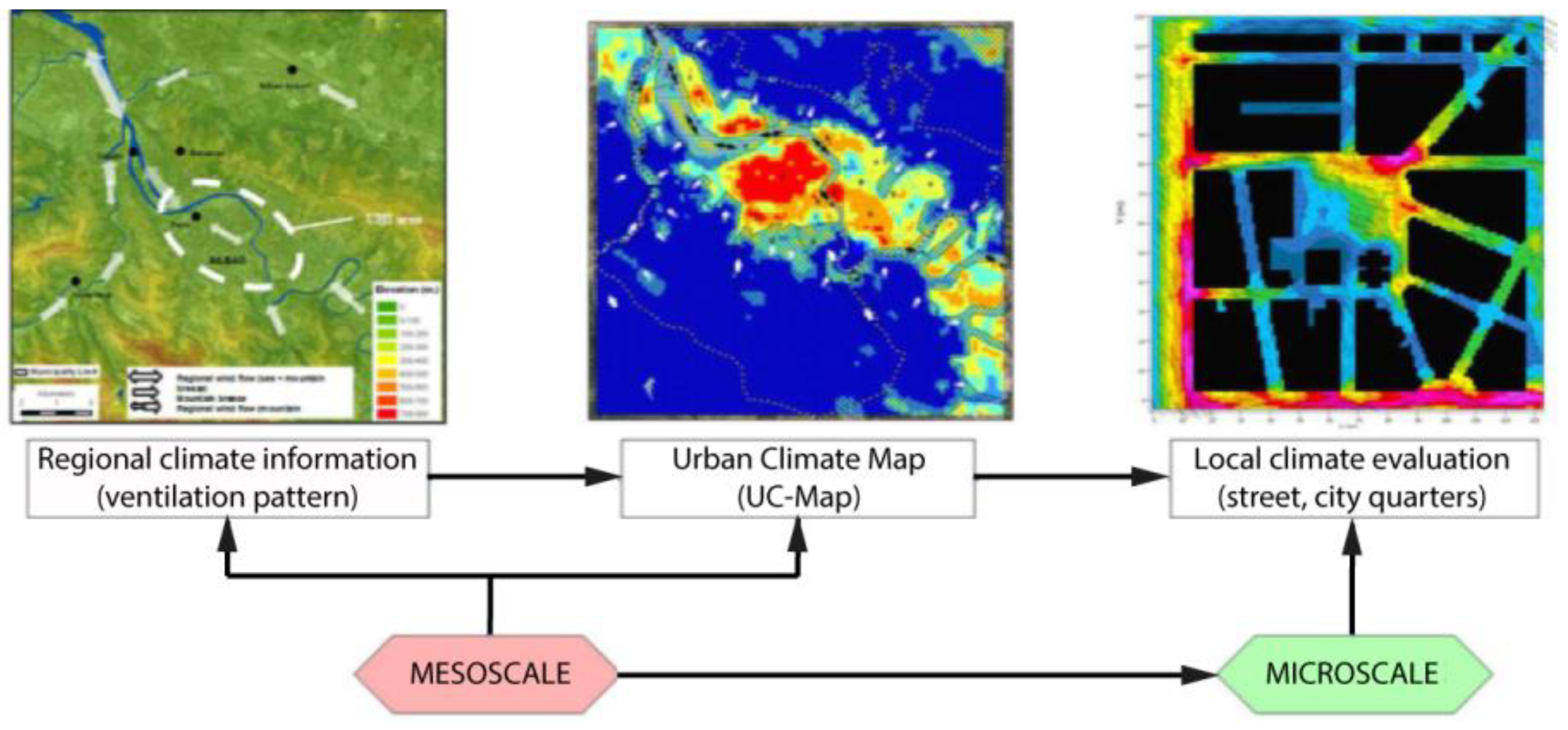
• Urban Climate Map (UC-Map). The UC-Map integrates urban climate factors within the strategies for urban developments, and it provides 2D data in spatial maps related to climate phenomena and hazards [57,58,59,60,61]. The UC-Map is characterized by two major components [35]: the first component is the urban climate analysis map (UC-AnMap), in which information on UHI effects and ventilation patterns is visualized, while the second component, the urban climate recommendation map (UC-ReMap), allows localizing critical sensitive climate areas in which mitigation and adaptation strategies for climate impacts are needed. The UC-Map is based on geographic information systems (GIS), which allow climate knowledge to be integrated into urban planning, and it has a typical resolution of 100 m [35,62].
• Environment-High-Resolution Limited Area Model (Enviro-HIRLAM). The Enviro-HIRLAM is an online model supported by the meso-meteorological (MetM) system that allows predicting atmospheric composition, meteorology, and climate change [63,64] by coupling modelling applications based on numerical weather predictions and an atmospheric chemical transport model (ACTM). This latter model allows regional- and urban-scale feedback between numerical weather prediction models and the ACTM [38,65]. Among the technical aspects, the system uses the nesting of domains for higher resolutions, different types of urbanization, and implementation of chemical mechanisms and aerosol dynamics. The Enviro-HIRLAM is also coupled with other modules such as a parameterization of the anthropogenic heat fluxes extracted from the large-scale urban consumption of the energy (LUCY) model [66] and the building effect parameterization module (BEP) [67]. The BEP is used to represent urban districts by underlying street urban canyons with constant widths but different heights and similar thermodynamic characteristics. Each surface of the urban substrate (street canyon floor, roofs, and walls of buildings) gives a contribution that is counted in the parameterization: the heat and turbulent kinetic energy equations are calculated independently as the main contributions of the vertical (building walls) and horizontal (floors and roofs) surfaces. The LUCY model is used to simulate the anthropogenic heat flux from the global- down to the individual-city-scale at 0.25 arc-minute resolutions [66]; moreover, data related to different working schedules, public holidays, traffic, and energy consumption can be included in the model.
• UrbClim. UrbClim has been developed for analysis of urban air temperatures and other climatic parameters for a city and its rural surroundings at a spatial resolution of a few hundred meters. In this model, the urban terrain is represented by an impervious slab characterized by parameters such as albedo, emissivity, and aerodynamic and thermal roughness length. A 3D atmospheric boundary layer module is coupled to this surface slab. Case studies have been conducted in Toulouse (France), Ghent and Antwerp (Belgium), Barcelona and Bilbao (Spain), London (UK), Almada (Portugal), and Berlin (Germany) to validate the model with respect to observed turbulent energy fluxes, wind speed, and urban–rural temperature differences, showing that UrbClim has an accuracy comparable to that of more detailed and complete models [42]. At the same time, the model is about two orders of magnitude faster than other high-resolution mesoscale climate models, ensuring UrbClim is suitable for long-time integrations required, e.g., in urban climate projections [42,68].

3.2. Tools and Models for Microscale Analysis

Smaller domains (a few hundred meters) and finer spatial resolutions (a few meters) are considered in the microclimate simulations: the typical grid scales ranging from street-canyon scale (less than 100 m) to neighbourhood scale (up to 1 km or 2 km). Therefore, at the microscale, the measurements and analyses are usually the most suitable to estimate local impacts and benefits in terms of human thermal comfort at the pedestrian level and the impacts of the different planning scenarios.

• Mobile measurements. Stationary networks of field stations and vehicles equipped with temperature sensors such as mobile measurements are some of the methods used for local climatological studies and to describe climate [69,70] and spatial variations in temperature [71,72]. Mobile platforms allow analysis of a large area in a relatively short period with the same instruments. Another key advantage is the analysis of temperature patterns in relation to topographical factors whilst avoiding large instrumental errors and calibration. Finally, the inclusion of surface temperature sensors for road climatological studies represents an important step in the development of the traditional mobile measurements [73].
• Observations: in-situ measurements and remote sensing. The in-situ-measurements derived from a technology allowing data acquisition from an object when its distance to the sensor is equal or smaller than any linear dimension of the sensor. Recently, new monitoring systems (i.e., remote sensing) coupled with wireless telecommunication technologies opened a new era in the measurement field with new network applications (i.e., network-wide data) to monitor, visualize, and transfer data to users via the Internet in real time [74].
• ENVI-met. ENVI-met is a 3D microclimate modelling software grounded in well-founded urban physics. It is based on coupled balance equations (including mass, momentum, and energy), which take into account the interaction between the different phenomena occurring in the urban environment. It is used to develop urban microclimate studies by reproducing the major processes in the atmosphere (i.e., air flow, turbulence, radiation fluxes, air temperature and humidity, vegetation, and water spray) and calculating meteorological factors and indexes for comfort quality within an urban area such as physiologically equivalent temperature (PET) and the predicted mean vote (PMV). ENVI-met has a high spatial and temporal resolution that allows a fine understanding of the microclimate at street-level. A typical horizontal resolution in ENVI-met varies from 0.5 m to 10 m, which is set for small-scale interactions between individual buildings, surfaces, and plants. ENVI-met can simulate microclimatic dynamics within a daily cycle in complex urban structures (i.e., buildings of various shapes and heights) and vegetation. Accordingly, ENVI-met is used by landscape architects and urban planners as a decision support instrument for urban recommendations in which contemporary demands of climate adaptation and mitigation aspects are considered. ENVI-met has been widely validated through numerous studies under various climate conditions, including temperate climates [75] and more extreme weather conditions [76,77,78]. ENVI-met has also demonstrated a good match with experimental data [79,80].
• TOWNSCOPE. TOWNSCOPE [51] is a digital system that supports urban decision-makers in conducting solar radiation access analysis to develop sustainable urban design strategies [81]. Coupled with solar evaluation algorithms, TOWNSCOPE allows the creation of a three-dimensional urban data system in terms of direct, diffuse, and reflected radiation in each surface point. TOWNSCOPE has also been coupled with a thermal comfort algorithm based on Fanger’s thermal comfort equations to provide climate data such as air temperature, relative humidity, ventilation rates, and wind speed for any point [82].
• RayMan. The RayMan model allows the study of complex urban structures by calculating the mean radiant temperature (T_mrt) from short- and long-wave radiation fluxes and their impact on a human energy balance model through the calculation of thermal indexes such as predicted mean vote (PMV) and physiologically equivalent temperature (PET) (presented in the next section) [52]. The urban physics of the RayMan model is grounded in the German VDI Guidelines 3789 Part II [83] (environmental meteorology, interactions between atmosphere and surfaces; calculation of short- and long-wave radiation) and VDI 3787 (environmental meteorology, methods for the human–biometeorological evaluation of climate and air quality for urban and regional planning. Part I: climate) [84]. Several experimental studies have been conducted to validate the tool [52].
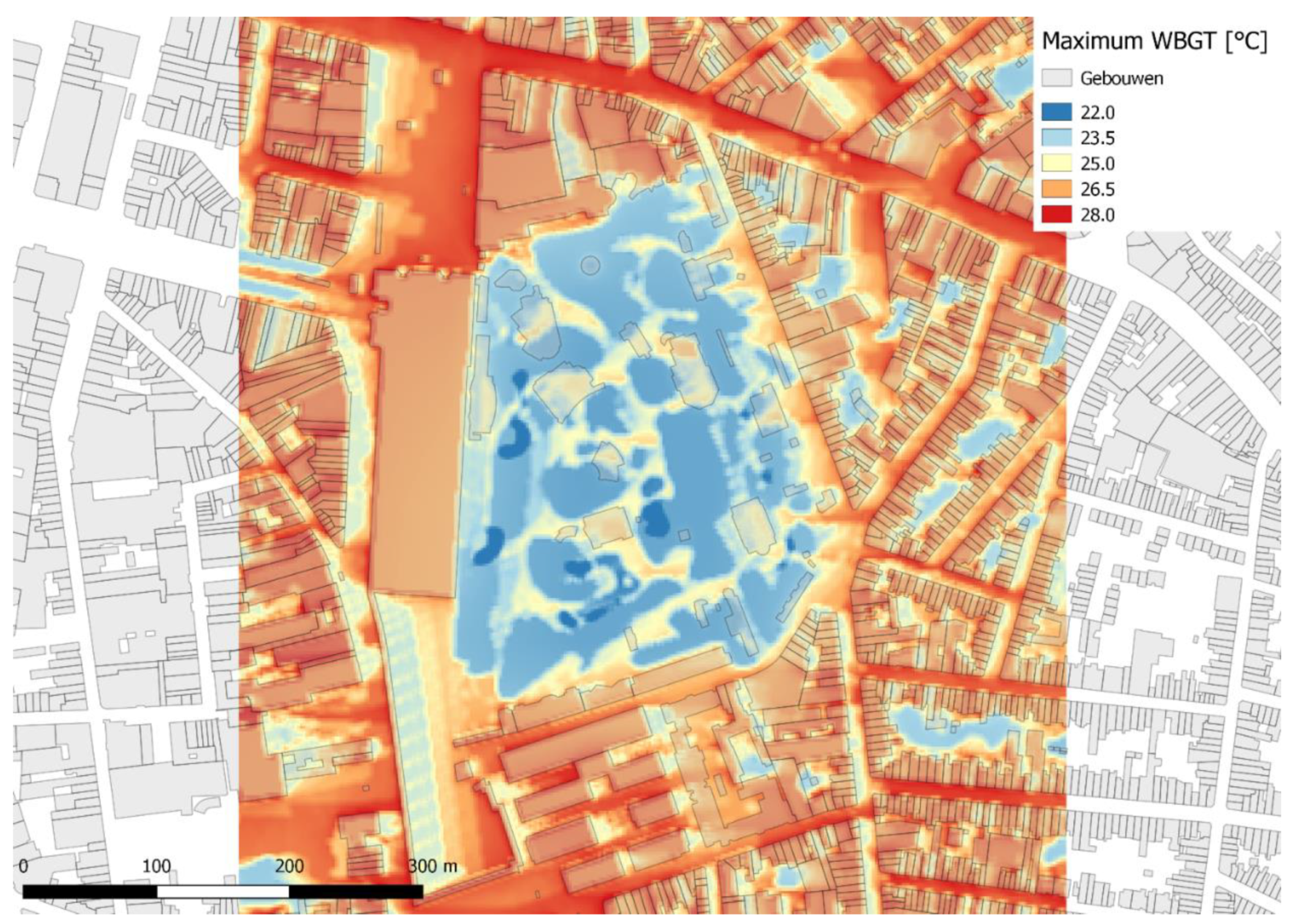
• UrbClim High Resolution (HR): In order to support local authorities with detailed heat stress analyses, VITO has developed a model tool to calculate a thermal comfort indicator (the wet bulb globe temperature (WBGT)) with a very high spatial resolution up to 1 m [85]. The WBGT is calculated by combining the standard output of the UrbClim model (see above) with detailed radiation calculations based on 3D building and vegetation data. The methodology is adopted from Liljegren et al. (2008) [86], which constitutes the recommended method to calculate outdoor WBGT values [87].

4. Indexes of Human Thermal Comfort

This section presents the thermal indexes used in the selected case study cities at the mesoscale and the microscale to evaluate human thermal comfort. For clarity, it is worth mentioning that the presented indexes are exemplary of the multitude of thermal indexes existing in the literature such as the UTCI and the mean thermal sensation vote (MTSV). The natural and artificial morphology have an influence on the climate parameters and conditions on both the mesoscale and the microscale. Their temporal and spatial impacts are significant at different levels (i.e., regional, district, and urban canyon) [52,88]. Furthermore, these factors also have an impact on the meteorological parameters such as air temperature, air humidity, wind velocity, mean radiant temperature, surface temperature and short- and long-wave radiation, which have a strong effect on the thermo-physiological conditions of humans [89,90]. All these parameters are considered in the energy balance of the human body, which is used in definitions of thermal indexes. The thermal indexes associate microclimate conditions with human thermal stress sensation, and they are categorized as steady-state models, despite some research demonstrating that they cannot effectively account for the dynamic aspects of human thermal adaptation [91].

• Physiological equivalent temperature (PET) and predicted mean vote (PMV). PET and PMV are thermal indexes to predict average human thermal responses. [20]. The PET allows evaluation of the human thermal comfort in both indoor and outdoor environments with the greatest spatial variability within a microscale urban area due to complex geometry and heterogeneous surface characteristics. It is expressed in degrees Celsius (°C) [4]. This makes PET comprehensible for all actors involved in the design process with or without a technical background. PET is equivalent to the air temperature at which, in a typical indoor setting, the heat balance of the human body is maintained with core and skin temperatures equal to those under the conditions being assessed. Its calculation is based on the Munich energy-balance model for individuals (MEMI) [89], which models the thermal conditions of the human body in a physiologically relevant way. This model takes into account the physics of the human body (e.g., gender, height, activity, clothing resistance for heat transfer, short-wave albedo, and long-wave emissivity of the surface) and the meteorological parameters (e.g., air temperature, air humidity, wind velocity, radiation fluxes, and mean radiant temperature) [89]. The PMV is based on the same method, and it is expressed as a dimensionless quantity that varies between −4 (too cold) and +4 (too warm). Its values can be linked to the percentage of people that feel comfortable at a given PMV value. The optimal value is 0, and at decreasing or increasing values, people increasingly feel uncomfortable. For both indexes to classify cold, neutral, and heat stress in urban canopies, the values refer to the evaluation scale of Matzarakis and Mayer [90].
• Land surface temperature (LST). LST is an index to assess the effects of surface radiative proprieties, energy exchange, internal climate of buildings, and human comfort. LST is usually coupled with other indexes, such as land-cover, land use, the vegetation index, and urban morphology [92,93,94,95]. For large domains such as cities, LST is typically determined by means of satellite remote sensing imagery. In Oltra-Carrió et al. [96], it emerged that the temperature–emissivity separation (TES) algorithm that retrieves LST data from satellite thermal imagery can best reproduce urban surface temperatures [97]. One advantage of this algorithm is that it does not require any background regarding the emissivity of the surface over urban areas. These models are characterized by strongly deviating infrared emissivity values, and the ASTER instrument on board the EOS-TERRA satellite platform is currently the only instrument that can employ this algorithm. ASTER imagery has a spatial resolution of 90 m in the thermal infrared part of the spectrum.
• Normalized difference vegetation index (NDVI). NDVI is defined as the ratio between (1) the difference and (2) the sum of the reflectance of the land surface in the red (ρ_red) and near-infrared (ρ_nir) spectral bands. Live green vegetation generally exhibits higher reflectance values in the near-infrared portion of the spectrum, so areas covered with vegetation yield high NDVI values. The normalization achieved by dividing the reflectance difference by its sum is mainly intended to reduce atmospheric effects as much as possible.
• Wet bulb globe temperature (WBGT). The WBGT has a long tradition of being used as a thermal comfort index and is the ISO standard for quantifying thermal comfort [98]. It is currently in use by a large number of bodies including the US and UK Military, civil engineers, sports associations, and the Australian Bureau of Meteorology [99]. Developed by the U.S. Army [100], the WBGT heat index has known temperature thresholds to characterize varying levels of human heat exposure, based on several observations.

5. Applications in Case-Study Cities

In this review work, the numerical models presented above were applied (i) at the mesoscale in the case study cities of Antwerp (Belgium), Rome (Italy), and Delhi (India) (

Table 2. Selected metrics and fixed settings for the case study cities analysed at the mesoscale.

Spatial Scale	City	Model/Tools	Index	Scenarios	Aim	Temporal Scale or Other Comments
Mesoscale	Antwerp	Satellite thermal image	LST	The best satellite image (least contaminated by cloud) was selected for analysis.	Map the surface UHI (SUHI). Analyse the effects of green infrastructure on LST.	24 July 2012 at 12:57 local time, registered using the ASTER instrument.
		UrbClim	Average daily mean and maximum and minimum air temperatures. Annual mean number of heatwave days (HWDs).	The expansion of the urban areas and the implementation of green areas in the city core in current and future climate conditions.	Assess the impact of different land-cover categories, in particular, those involving urban vegetation. Set limits to what can be maximally achieved by greening the city.	20-year periods (1986–2005, 2041–2060, and 2081–2100) with a focus on the summer period (June–August).
Mesoscale	Rome	UrbClim	Average daily mean and maximum and minimum air temperatures.	Simulations were performed for climate-change scenarios RCP4.5 and RCP8.5	Assess the impact of climate change on air temperatures and heat stress.	30-year periods (1987–2016 and 2036–2065)
Mesoscale	Delhi	Land-cover categories contained in the World Urban Database and Access Portal Tools. MODIS instrument on board the TERRA platform.	LST, NDVI, and WBGT	The NDVI and LST were observed as an average for the measured month (February 2015). WBGT measurements were procured from station observations and were used for the purpose of model validation.	Review the impact of vegetation abundance.	February 2015

) and (ii) at the microscale in the case study cities of Antwerp and Bilbao (Spain) (

Table 3. Selected metrics and fixed settings for the case study cities analysed at the microscale.

Spatial Scale	City	Model/Tools	Index	Scenarios	Aim	Temporal Scale or Other Comments
Microscale	Antwerp	In-situ measurements	Air temperature	One station was installed in the centre of the city, one at a rural location near Antwerp, and a third one in the city’s main centrally located park, called the Stadspark.	Assess the benefit of urban greening on thermal comfort in urban environment.	The data were acquired during the summer of 2013 (from 10 July to 11 September).
		Mobile measurements	Air temperature	The car was driven along a trajectory starting at the bio farm (rural) station at 19:17 and crossing the entire city up to the harbour area (arrival there at 20:21), passing near the Stadspark in the process.	Measure the daytime maximum air temperature along the designed path.	Car equipped with a number of sensors, including actively and passively ventilated temperature sensors.
		UrbClim HR	WBGT	The simulation experiments were conducted for the neighbourhood of the Zoo of Antwerp.	Investigate the local heat stress situation on a typical hot summer day.	A typical hot summer day (24 July 2012).
Microscale	Bilbao	ENVI-met	PET	Initial scenario, different ground materials and greening scenarios using grass, tree-lined streets.	Comparative analysis of green actions to improve outdoor thermal comfort inside typical urban street canyons.	The evaluation was performed in three urban street canyons characterized by different aspect ratios: a height/width (H/W) ratio of 1.3 “compact low-rise” exemplified by Casco Viejo, H/W 1.5 “compact mid-rise” exemplified by Abando/Indautxu, and H/W 3.5 “open-set high-rise” exemplified by Txurdinaga. The analysed scenarios were run on 6 August and 7 August to simulate typical summer day conditions in Bilbao.
				Different orientation and greening strategies maintaining the following constant ratios: Htree/Hcanyon and Wtree/Wcanyon.	Generalization of the first part of the work analysing the effects of orientation, aspect ratio, ground surface material, and vegetation elements on thermal stress inside typical urban canyons.

). The analyses in the selected case study cities were performed within two European research projects where researchers (i.e., the authors of this study) in collaboration with urban stakeholders and public authorities worked together to define: (i) the objectives of the type of analyses to be conducted, (ii) the selection of the most suitable model or tool to be used, (iii) the process and the discussion of the outcomes, and (iv) the transfer of the outcomes of the analyses into urban planning strategies or recommendations to mitigate the climate risk of UHI in built environments.

5.1. Mesoscale Applications

In this section, the main outcomes on the case-study cities at the mesoscale are presented.

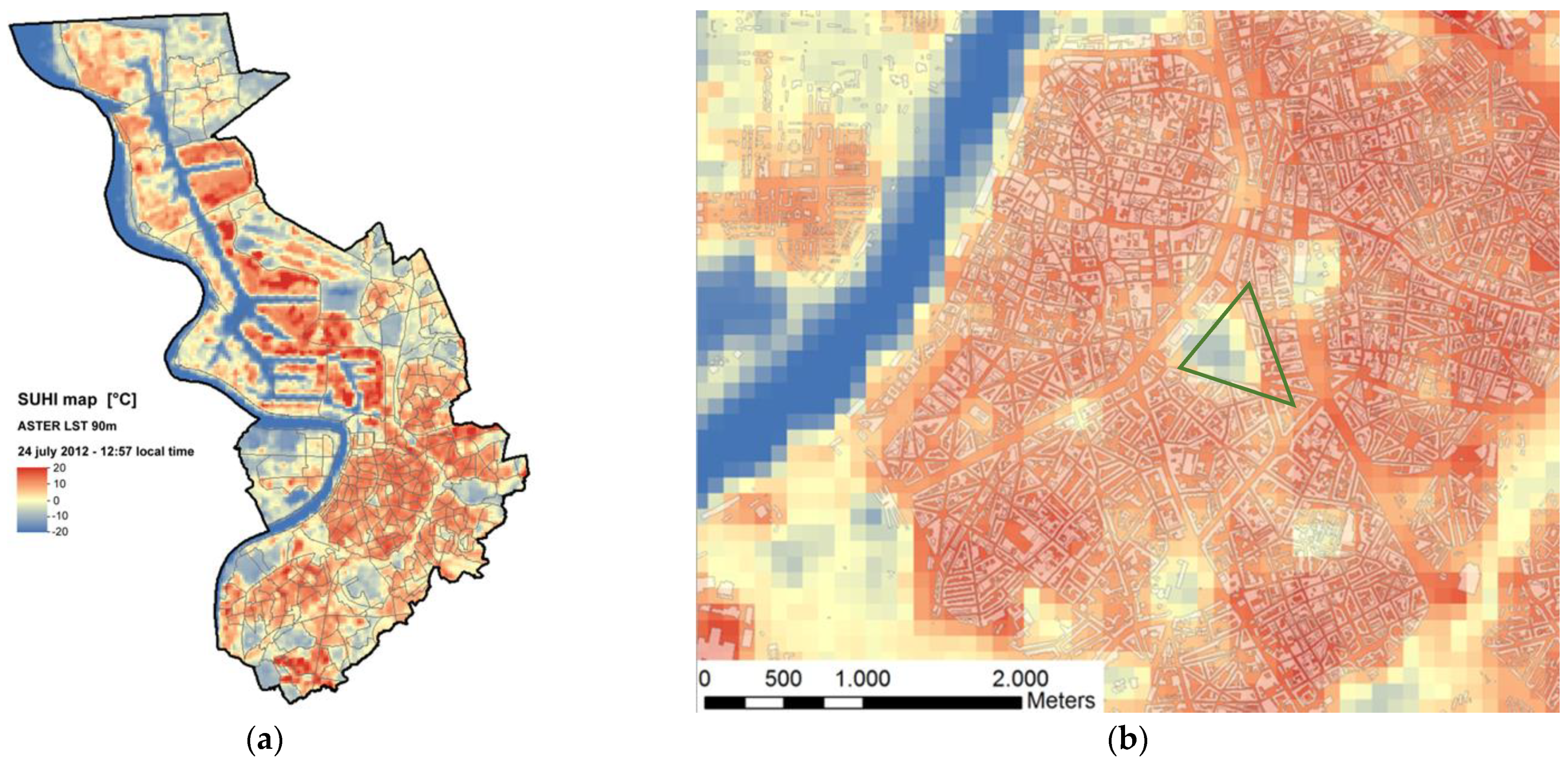
• Antwerp. In the case study city of Antwerp, the surface UHI was mapped using thermal infrared satellite imagery in order to (i) evaluate the effect of the vegetation on LST and (ii) the relationship between the LST and the peculiarities of urban surface cover. Through the Earth Remote Sensing Data Analysis Center (ERSDAC), several cloud-free ASTER images during the summer were selected. The ASTER LST image of 24 July 2012 (Figure 2a) shows that the UHI effect of Antwerp is clearly present in the densely built-up areas of the city, which were warmer than the rural surroundings mostly covered by vegetation. The harbour area also stands out distinctly as a local hotspot. The difference in terms of peak temperature were several tens of °C. The areas most affected by high temperatures were mainly characterized by large, open industrial terrain, with large flat asphalt or concrete surfaces and roofs covered by dark roofing material. However, there was a triangular area in the centre of Antwerp that had lower temperatures (Figure 2b) due to the presence of the Stadspark (green triangle in Figure 2b), which is the major urban park near the city centre. LST values in the park were up to 15–20 °C cooler than in the surrounding densely built-up areas.

Another part of the study conducted in Antwerp focused on model-based land-use change experiments. Several scenarios were simulated with the UrbClim model for 20-year periods (1986–2005, 2041–2060, and 2081–2100), focusing on the average daily mean and the maximum and minimum temperatures for the summer period (June–August). The reference situation, using the observed vegetation cover fraction, was compared with a scenario in which the amount of urban vegetation was set to 60%. The results showed that this strong greening of the city had an effect of up to 2 °C on the average temperatures, which is consistent with reported measurements and modelling studies. This may not seem much, but it is significant with respect to the average UHI effect of around 3 °C. The impact on the number of heatwave days (HWDs) is comparable, with a reduction of 1.5 days per summer compared to average city centre HWD values of around 2. Regarding the simulations of future conditions, the UHI effect of the city of Antwerp was found to be fairly constant under future climate conditions, whereas the number of HWDs is projected to increase almost tenfold by the end of the century under RCP8.5.

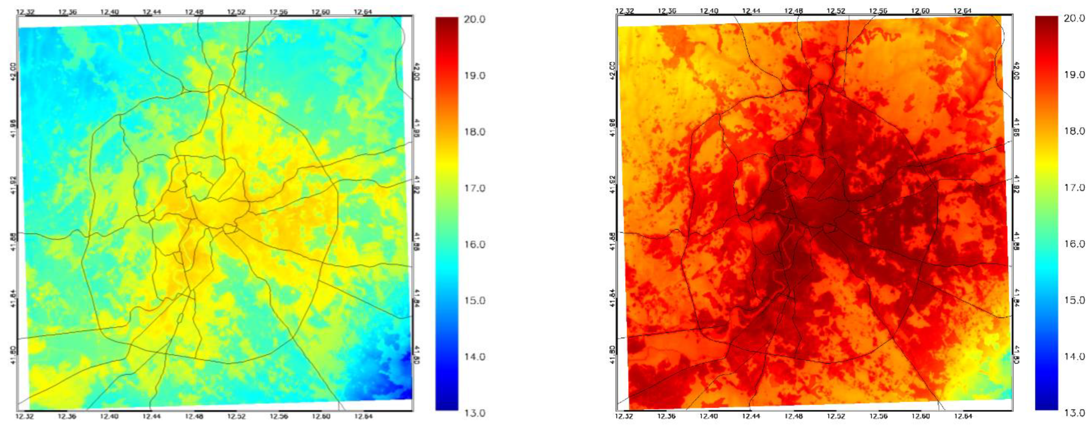
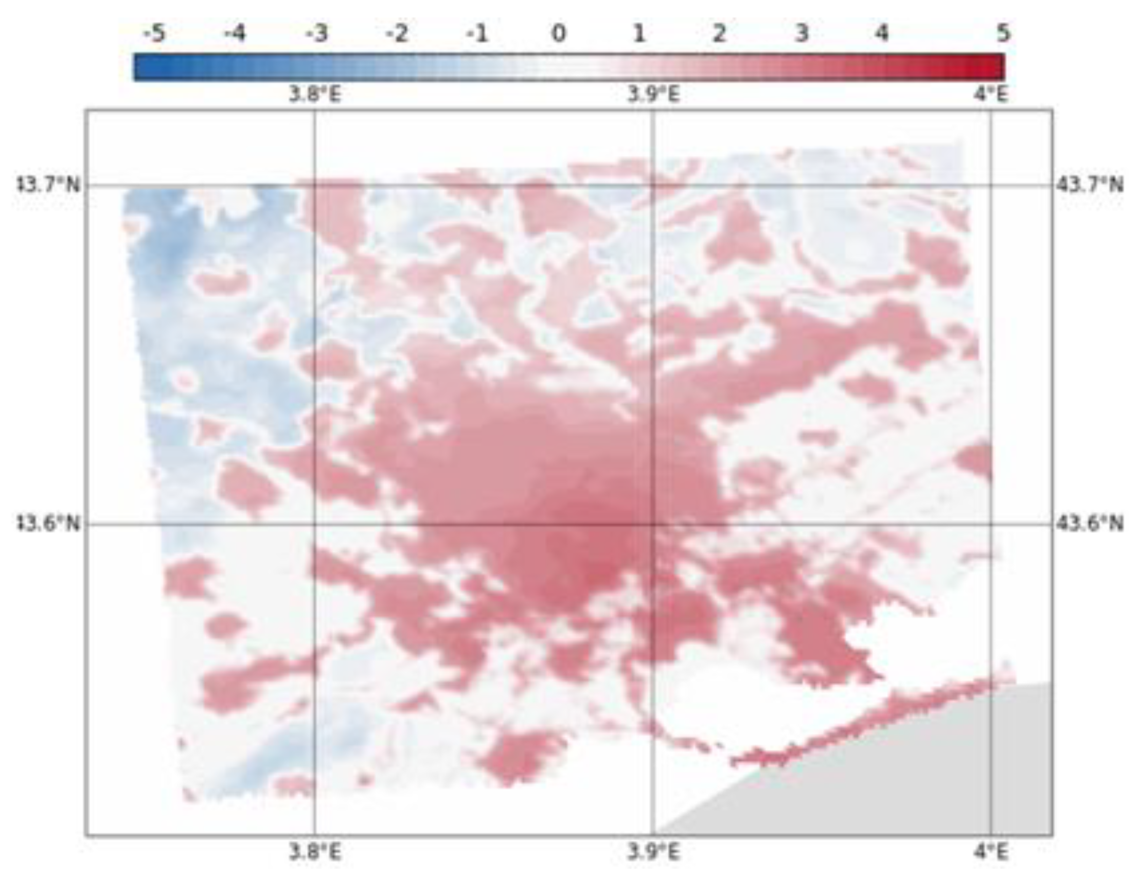
• Rome. In Rome, the impact of several climate change scenarios on air temperatures and the UHI was assessed with the UrbClim model in the framework of the EU-H2020 Climate-fit.city project. A thirty-year historical period (1987–2016) was simulated with the model, driven by ERA5 reanalysis data. To generate future climate scenario timeseries, a statistical downscaling methodology was applied in which all available results from the CMIP5 archive were used to derive the local climate change signal. This signal was used to perturb the historical timeseries, following the quantile delta perturbation method. This downscaling method intrinsically involves bias correction, i.e., the removal of any systematic difference between the climate model outputs and the historical observations. The result of the perturbation-based statistical downscaling are timeseries of the same length and time scale as the historical time series but following future climate conditions. In this way, it is possible to rather quickly generate several climate scenarios while taking into account a large number of driving global climate models. A more-detailed description and a validation of the methodology can be found in Lauwaet et al. (2015) [68]. Figure 3 shows an example result of the analysis in which the current and mid-century air temperatures are compared. Clearly, air temperatures are expected to increase significantly in Rome in the next decades by 2–3 °C on average. Conversely, the intensity of the UHI is not expected to change significantly unless land-use changes are considered.
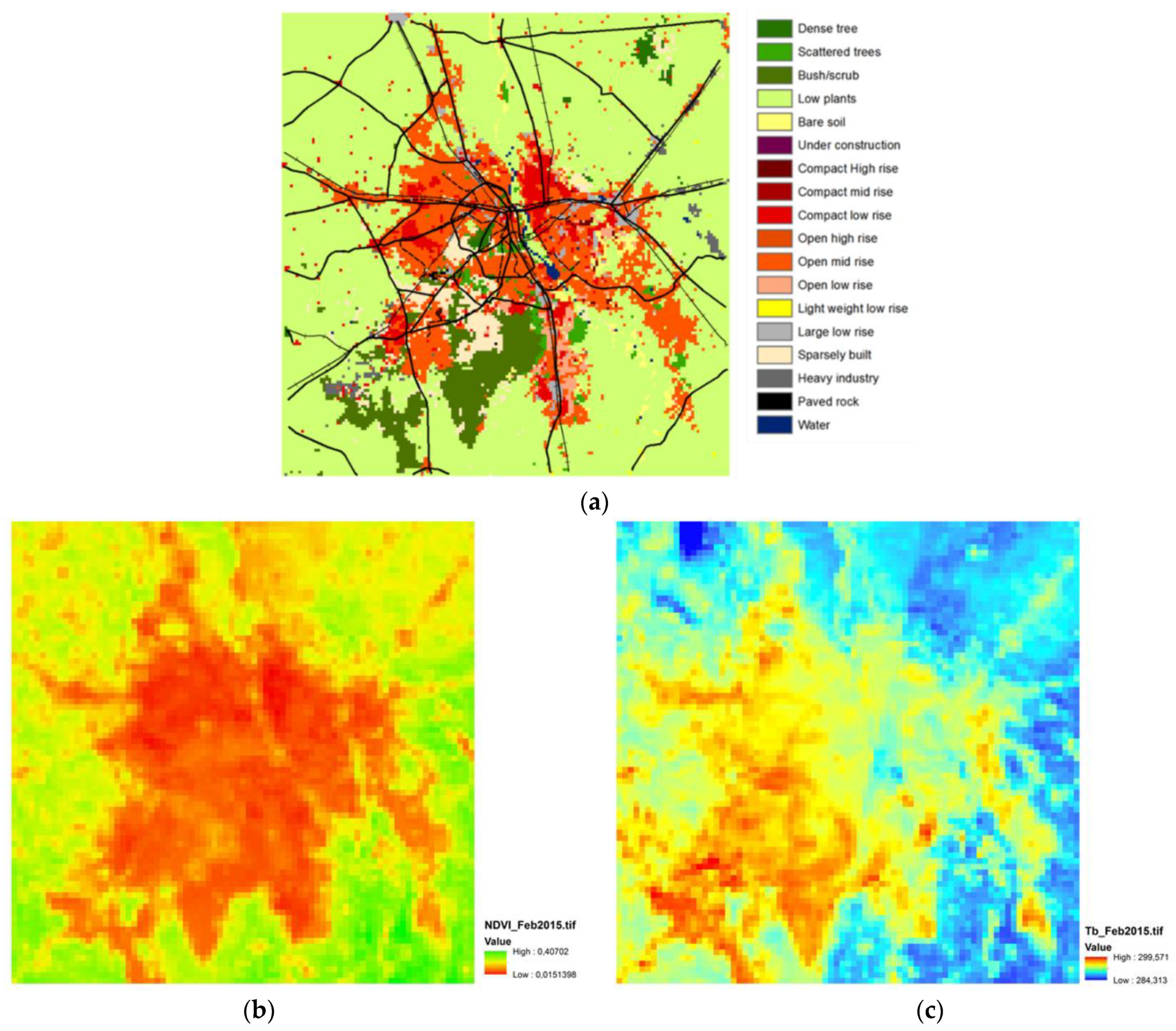
• Delhi. Similarly, it was confirmed in the case study of Delhi by using land-cover categories contained in the World Urban Database and Access Portal Tools and the MODIS instrument onboard the TERRA platform. The analysis, conducted in February 2015, was based on the two quantities, NDVI and LST. The outcomes demonstrated that the presence of larger green areas is preferable given their higher cooling effect rather than the presence of several distributed green spots. In Figure 4a, the LST map for February 2015 shows that the urban portions of the domain exhibited higher LST values. Furthermore, the comparison between NDVI/LST images shows that an inverse relation exists between the two, i.e., areas with sparse vegetation cover exhibit the higher temperatures, and vice versa. This is visible even in smaller structures, such as in the quasi-linear feature extending in the upper-right corner of the images contained in Figure 4b,c. The further analysis is straightforward: a regression line linking the LST linearly to the NDVI was calculated, as shown in Figure 5. This regression analysis quantitatively confirms the inverse relationship between both quantities, with a slope of around 5 °C between the bare (NDVI = 0) and greener (NDVI ≈ 0.4) portions of the domain. The correlation between both quantities in the considered situation amounts to r = 0.67.
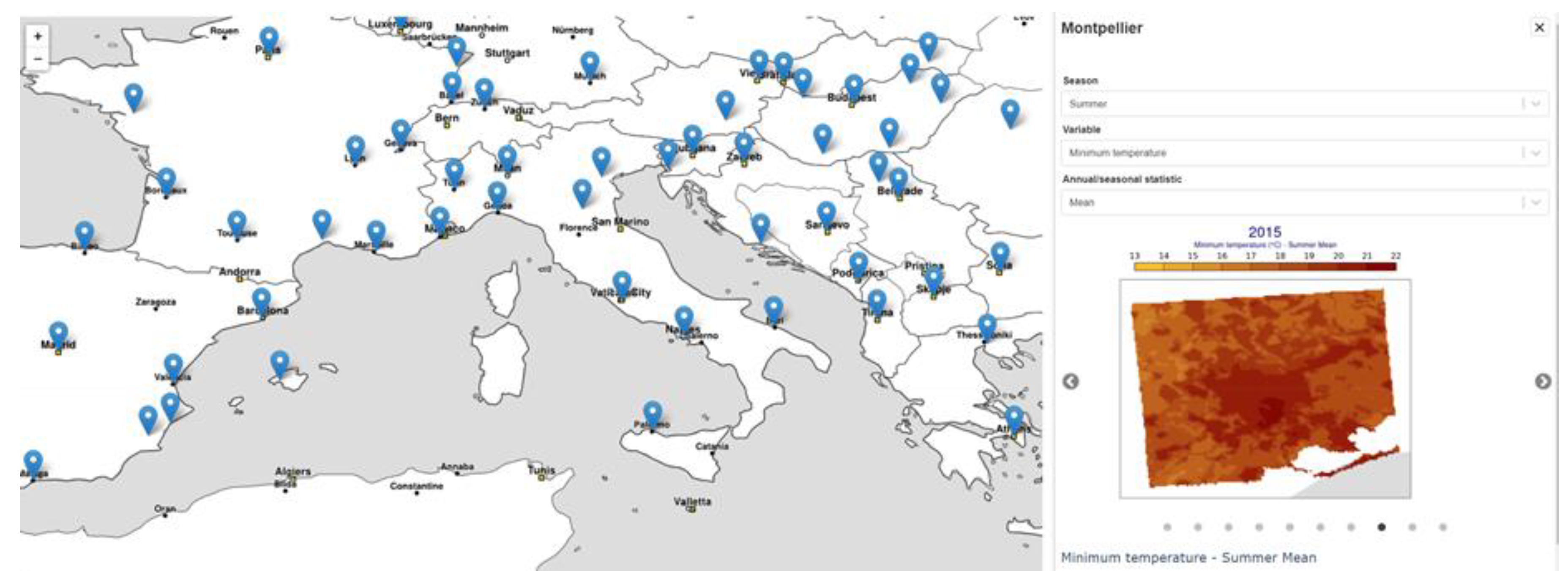
• European cities. The UrbClim model was employed to generate an online data archive and interactive query dashboard containing mesoscale urban climate information for 100 European cities, several tens of which are located in the Mediterranean (Figure 6). While this does not constitute a case study properly speaking, it is presented here given its value for the broader urban climate research community. Indeed, this freely accessible online archive, established within the Copernicus Climate Change Service (C3S), constitutes a valuable resource for the analysis of inter-city variability of UHI characteristics. The downloadable data contained in this archive have the following characteristics:
  • One hundred cities across Europe were included, several are in the Mediterranean.
  • Forced by ERA5 large-scale model output.
  • Georeferenced data at 100 m spatial resolution.
  • Ten-year period covered (2008–2017) at hourly temporal resolution.
  • Variables: near-surface (2 m) air temperature, specific humidity, and wind speed.
  • Ancillary variables: land–sea mask and rural–urban mask.
  • Fully documented data characteristics and a description of data processing.
  • Freely downloadable NetCDF files (C3S, 2021b).

The C3S [101] also hosts interactive online dashboards allowing to screen a subset of the urban climate data [102,103]. An excerpt of the dashboard is shown in Figure 6, while Figure 7 provides an example of the UHI intensity for the city of Montpellier (France).

5.2. Microscale Applications

At the microscale, the case study cities of Antwerp and Bilbao were analysed.

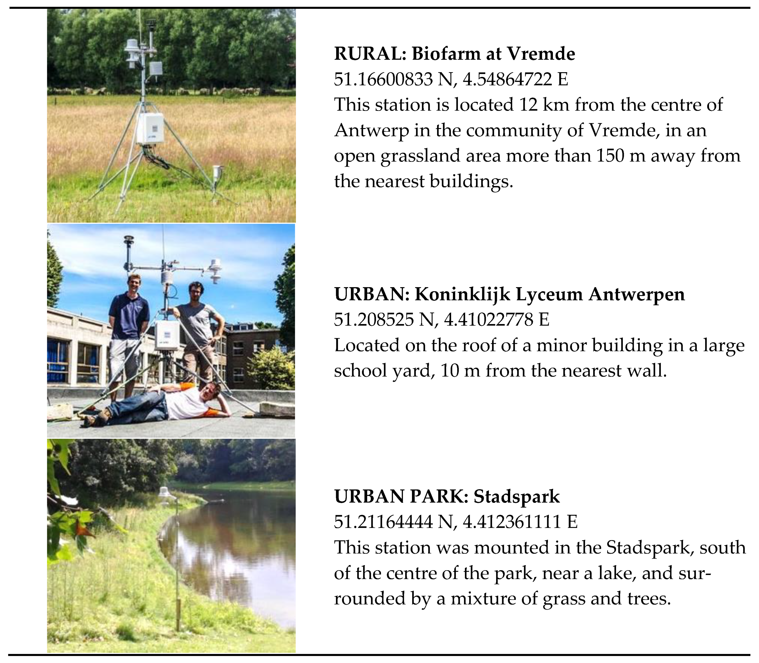
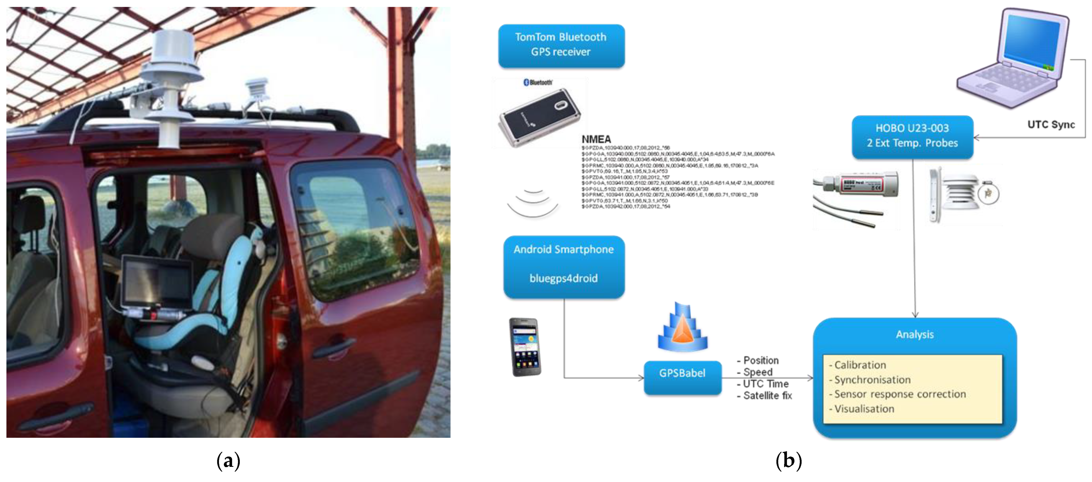
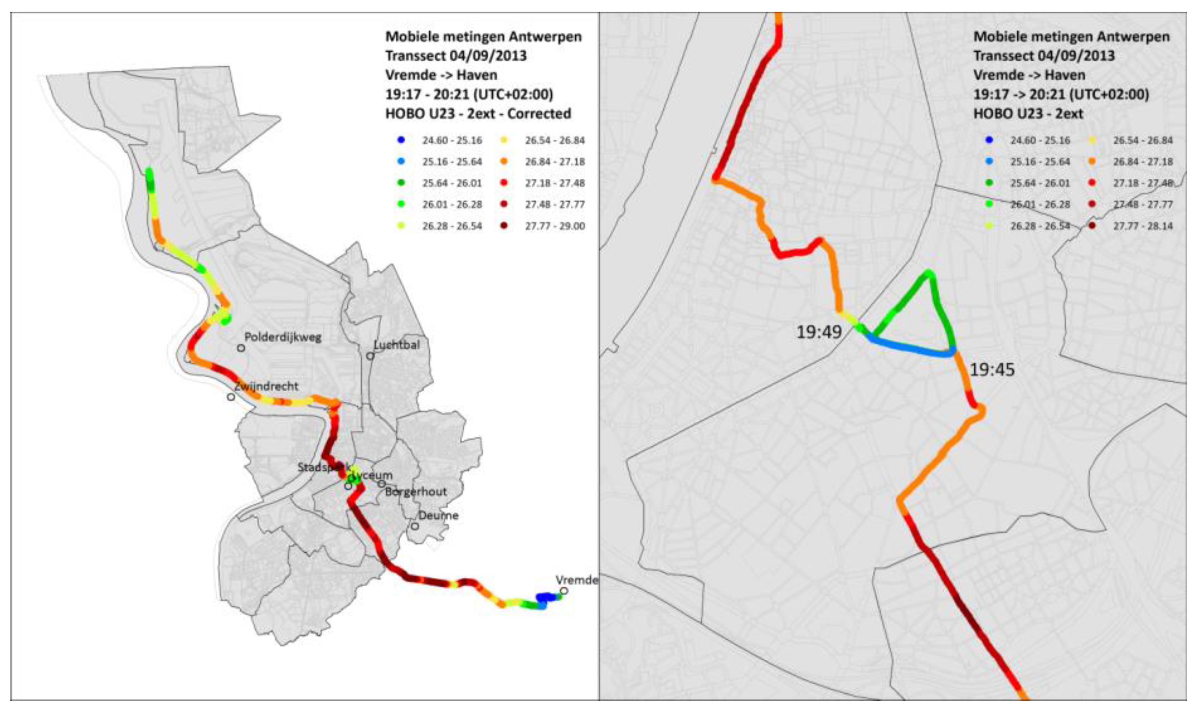
• Antwerp. In Antwerp, a series of in-situ and mobile (car) measurements were conducted to provide evidence of the impact of greenification on temperature. Several stations in and near Antwerp were installed: one in the centre of the city, one at a rural location near Antwerp, and a third in the city’s main centrally located park, the Stadspark. For the in-situ measurements, an air temperature sensor of the highly accurate RTD type (PT1000) was used, housed in an actively ventilated radiation enclosure (43502 Aspirated Radiation Shield, Young Model type) (Figure 8).

The data, acquired during the summer of 2013 (from 10 July to 11 September), considered the average diurnal cycle of the urban–rural temperature differences. The urban station exhibited the strongest average UHI magnitude, with values below 1 °C during the day and exceeding 3 °C at night. The cooling effect of the park was evident both during the day, when the UHI effect nearly vanished, and during the night, when it was between 2 °C and 2.5 °C. On average, the temperature in the park was more than 1 °C below the urban (Lyceum) station. This cooling effect was also confirmed by the reduced number of nights during which the temperature did not drop below 18 °C or 20 °C. Indeed, while in the central urban location (Lyceum), the temperature exceeded the 18 °C (20 °C) nocturnal thresholds on 13 (6) days (out of a total of 63 observation days), while the Stadspark station recorded 9 (2) days. The rural location exceeded these temperatures on only 2 (0) days (

Table 4. Mean UHI statistics for the urban and urban park stations, separately for day- (10–18 h local time) and night-time (22–4 h). The two rightmost columns give the number of nights with minimum temperature values exceeding the thresholds of 18 °C (nocturnal minimum temperature used in the definition of a heatwave day in Belgium) and 20 °C (which defines a “tropical night”), respectively.

Station	Site Type	UHI Day Mean (°C)	UHI Night Mean (°C)	# Nights Tmin > 18 °C	# Nights Tmin > 20 °C
Lyceum	Urban	0.74	2.94	13	6
Stadspark	Urban park	0.06	1.85	9	2
Bio farm	Rural	-	-	2	0

).

Other measurements were conducted with a car equipped with sensors, including actively and passively ventilated temperature sensors (Figure 9). Temperatures from HOBO temperature sensors were synchronized with data from a GPS receiver to obtain an accurate positioning of each measurement. The data-processing chain is graphically depicted in Figure 9. During the trajectory of one hour, an overall cooling rate of the order of 1 °C was estimated, which needed to be corrected for, as otherwise the final stretches of the trajectory would appear to be miraculously cooler for the wrong reason (i.e., not related to any landscape feature). Consequently, the background cooling rate was corrected for by adding a temperature increment proportional to the elapsed time.

The car was driven along a trajectory starting at the bio farm (rural) station (starting time: 19:17), crossing the entire city up to the harbour area (arrival time: 20:21) and passing along an edge of the Stadspark. This trajectory was run late in the afternoon of 4 September 2013, a late summer day with daytime maximum temperature values near 29 °C, to acquire the temperature variation data over this trajectory (Figure 10). The urban–rural temperature gradient and the cooling effect of the Stadspark were clearly evident, with temperatures of 1–2 °C lower than those in the nearby densely built urban areas.

In the framework of the EU-H2020 Climate-fit.city project, microscale simulation experiments were conducted by using the UrbClim High Resolution WBGT model for the Zoo of Antwerp (Figure 11).

The goal of the simulations was to assess the local heat stress situation in the Zoo and the benefits of the trees and ponds on the local thermal comfort. We focus here on the daily maximum WBGT values for a typical hot summer day. Clearly, the Zoo is a cool spot in the neighbourhood as its tree crowns and small ponds provide cooling that keep the WBGT values up to 6 °C cooler than on sealed surfaces where there is no shade. In these non-shaded and non-vegetated locations, WBGT values reach up to 28 °C, which corresponds to “high heat stress” conditions, whereas for shaded and vegetated locations, the WBGT values stay below the heat stress threshold of 25 °C.

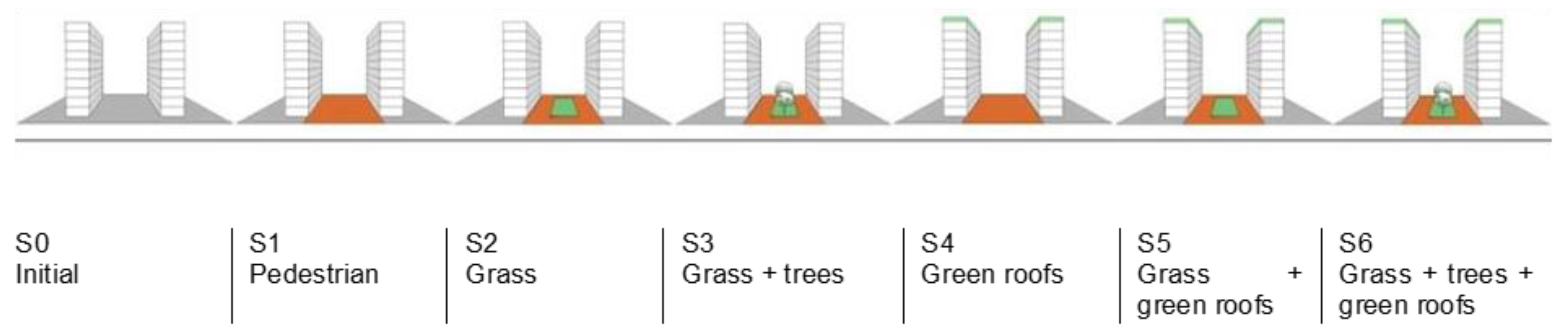
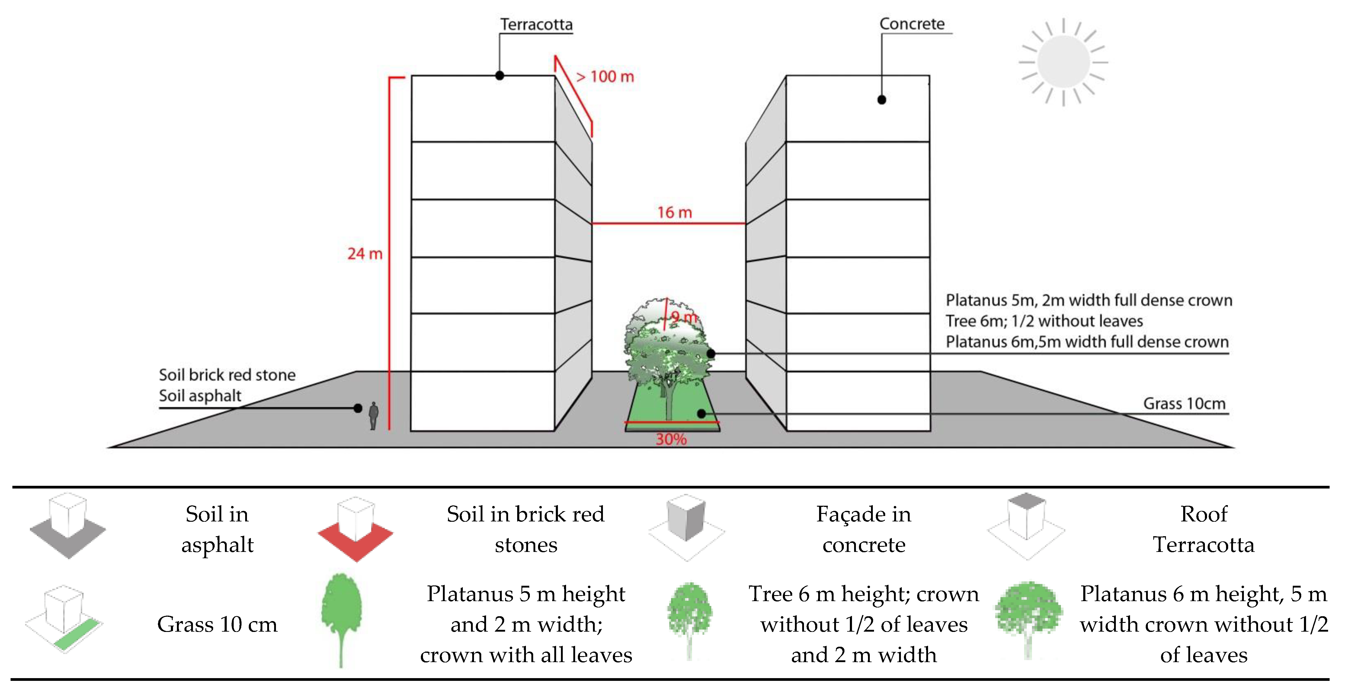
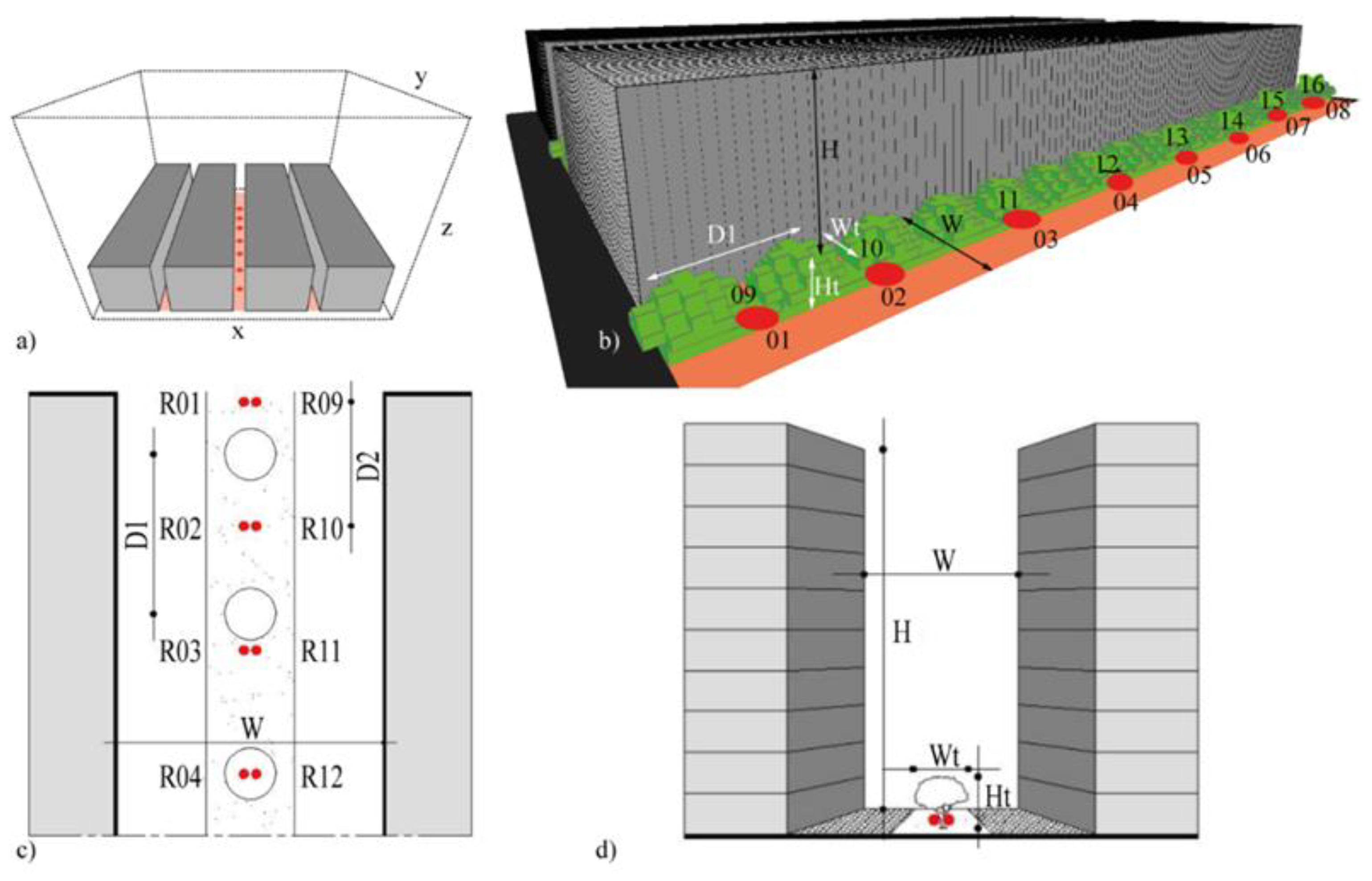
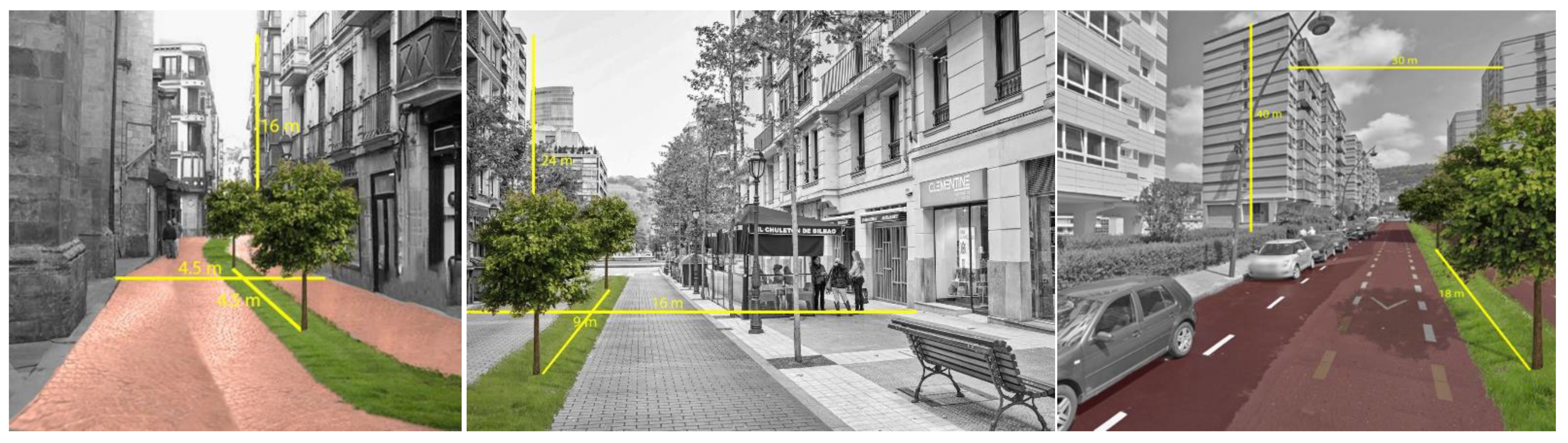
• Bilbao. The analyses conducted in Bilbao were run in ENVI-met, and they consist of two series of comparative analysis for green actions to improve outdoor thermal comfort inside three urban areas that are the most affected by the risk of a heatwave and that are the hottest in the city of Bilbao [2,30].

In the first series of analysis [2], seven scenarios were analysed: the current situation characterized by soil in asphalt for vehicular traffic (S0); the reconversion into pedestrian streets with red brink stones (S1); and different applications of vegetation elements such as grass (S2), grass and trees (S3), green roofs (S4), and combinations of these (grass and green roofs (S5) and grass, green roofs, and trees (S6)) (Figure 12).

The assessment was performed in three typical urban street canyons characterized by different aspect ratios, height/width (H/W) ratios, and urban features (Figure 13):

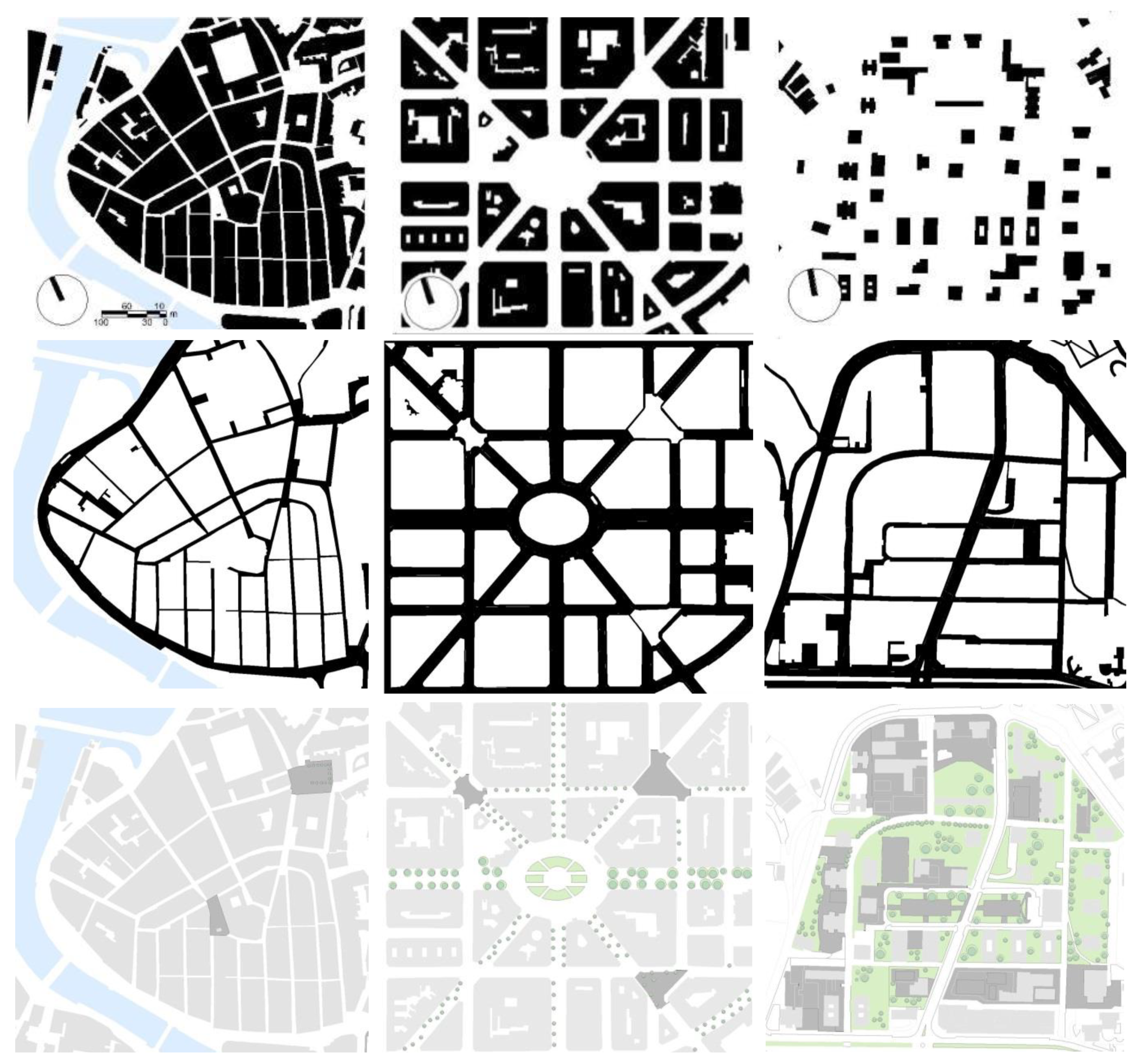
• Compact low-rise (i.e., Casco Viejo), H/W = 1.3: buildings are generally residential; commercial blocks are of four to six stories and are mostly attached to one another. The area is typical of the historical area of the city, which is characterized by high density and narrow streets. No green areas are present.
• Compact mid-rise (i.e., Abando/Indautxu), H/W = 1.5: buildings are generally seven/ten stories high. It is a typical residential and commercial high-density area in the city centre with attached buildings. Streets are mostly narrow with one traffic and parking lane, but wider avenues of four traffic lanes are also present. Green areas are scarcely present.
• Open-set high-rise (i.e., Txurdinaga/Miribilla), H/W = 3.5: buildings are generally high-rise housing blocks with more than nine stories. Open spaces and green areas are common around the buildings.

The impact of the different scenarios was estimated with the PET index. In that regard, vegetative measures, which were applied inside the street canyons such as tree-lined streets, had a noticeable cooling effect at the pedestrian level in terms of PET local spatial reduction. The strongest reductions of 10 °C in air temperature were found inside and specifically under the tree crowns in scenario S6. The effect of the green roofs (S4) on PET in the street canyon was also noticeable but relatively small compared to the presence of grass and trees (S3). In the centre of the street canyons, the cooling effect from a green roof was not found in compact low-rise urban areas, whereas it had low influence in the street canyon of compact mid-rise and open-set high-rise (<1 °C). However, for perpendicular or oblique winds, the cooled rooftop air may have become entrained into the street canyon and resulted in noticeable PET reductions. However, more dedicated analyses are necessary to study this effect. The combination of all green elements (S6 trees, grass, and green roofs) showed the largest impact on the PET levels.

Another relevant outcome relates to the thermal effect created by the installation of different finishing materials for the ground. For example, in Bilbao, the increased intervention to convert streets into pedestrian promenades by replacing the asphalt with decorative red brick stones increases the values of mean radiant temperature and surface temperature and consequently the PET level at the ground level. Finally, both aspect ratio and orientation were found to have a considerable influence on the street’s thermal comfort in the urban environment and consequently on people’s thermal sensation. In all urban areas, for the NE–SW orientation, the solar radiation had the highest impact on thermal discomfort at the pedestrian level. Only in open-set high-rise urban areas, the presence of the trees locally reduced the human thermal stress at the pedestrian level.

To generalize the impact of orientation, aspect ratio, and combined vegetation elements, a second set of analyses was conducted in the typical urban street canyon of Bilbao [3]. The materials were set to reproduce the real materials of walls, roofs, and soil, which are typically used in the analysed urban areas (

Table 5. Settings of materials and vegetation elements applied in the ENVI-met model.

Surface	Buildings		Street/Path		Soil
	Walls	Roofs	Pedestrian Path	Vehicular Path	Under Building	Under Grass
Description	Brick	Tile	Red brick stones	Asphalt road	Concrete (used/dirty)	Loamy soil
Thickness (m)	0.15	0.10	2	2	2	2
U-value (W/m2K)	0.44	0.84	NA	NA	NA	NA
Albedo	0.20	0.30	0.30	0.12	0.40	0.00
Vegetation element	Grass			Trees
Installation	Street			Compact low-rise	Compact mid-rise	Open-set high-rise
Trees and density	Average density			Platanus with 2/3 of full-fill crown’s density
Height (m)	0.1			4	6	10
Width (m)	30% of the street’s width			1.5	4.5	6
Albedo	0.30			0.6	0.6	0.6

). For the vegetation elements, 30% of the total street’s width was covered by grass with a height of 0.1 m. The foliage of the trees’ crown was set equal to 2/3 of the full-fill density (Table 5) (Figure 14).

The distance between the aligned trees (D1) was set to maintain a constant ratio of foliage coverage (D1/Wt). Fourteen receptors were set in the central part of the street canyon equidistant from each other (D2) to assess the thermal comfort through the PET index at 1 m high from the ground. The spatial distribution of the receptors was set to study the local benefits due to the presence of the trees: some receptors (e.g., R02, R09) were located between the trees and others (e.g., R04 and R12) under the trees’ crown (Figure 15). All model settings for building blocks were set to generalize the geometry of the analysed urban areas and to facilitate the replicability of the methodology in different parts of the city where geometric characteristics (H/W and B/T) and vegetation elements are similar.

The comparative analysis was conducted in four scenarios reproducing the typical orientations of the selected urban areas (S0): 24° North–South (N-S) in Casco Viejo; 17° N–S in Abando Indautxu; and 9° N–S in Txurdinaga/Miribilla.

In the second set of simulations, four standardized orientations (S1) such as N–S, East–West (E–W), North-east–South-west (NE–SW), and South-east–North-west (SE–NW) for the selected urban areas were analysed to study the impact of street pavement material when changing from asphalt (albedo = 0.12) to pedestrian boulevards with red brick stone (albedo = 0.30). Since the last decade, these interventions are typical in Bilbao, especially in compact mid-rise and open-set high-rise urban areas. Whereas, in the historic centre of Casco Viejo, a compact low-rise urban area, the decorative red brick stones were originally used as pavement material. No vegetation elements were set.

In the last set of simulations, the vegetation elements were added (Scenarios M01 and M02) without giving any obligation or disposition to dwellings’ owners and designers for interventions at the building level. The scenarios were characterized by a loamy ground soil positioned in the central part and covering 30% of the street’s width, while the rest of the street was covered with red brick stones. The loamy soil included the presence of grass, while a tree-lined stripe was set in the central part of the street (

Table 6. Settings of the scenarios M01 and M02 to study the effect of the vegetation elements.

Urban Area	Streets’ Pavement	Orientations	Grass on the Street	Trees	Scenario M01		Scenario M02
					Ht/H	Wt/W	Ht/H	Wt/W
Compact low-rise	Red brick stone	N–S, NE–SW, SE–NW, E–W	0.10 m	Tree 4 m; 1/2 without leaves	0.25	0.30	0.25	0.30
Compact mid-rise				Tree 6 m; 1/2 without leaves	0.25	0.28	0.25	0.30
Open-set high-rise				Tree 10 m; 1/2 without leaves	0.25	0.18	0.25	0.30

).

In

Table 7. Summary of the most relevant and critical results for the different scenarios in the compact low-rise urban areas.

Indicators for Heat Stress in Compact Low-Rise Urban Areas
Scenario	Standardized Orientations-S1		Mitigation-M01		Mitigation-M02
Orientation	North-east–South-west	North-west–South-east	North-east–South-west	West–East	North-east–South-west	West–East
Intensity Peak value of PET
	The peak value was equal to 52.97 °C, and it was reached at 4:30 p.m.	The peak value was equal to 32.94 °C, and it was reached at 12:30 p.m.	The peak value was equal to 47.17 °C, and it was reached at 4:20 p.m.	The peak value was equal to 30.97 °C, and it was reached at 10:30 a.m.	The peak value was equal to 45.84 °C, and it was reached at 4:20 p.m.	The peak value was equal to 30.32 °C, and it was reached at 10:30 a.m.
Duration of PET intensity Hours of peak values of PET
	The highest values of PET were higher than 49 °C and persisted from 3:30 p.m to 4:30 p.m.	The highest values of PET were higher than 32 °C and persisted from 12:10 p.m to 1:10 p.m.	The highest values of PET were higher than 42 °C and persisted from 3:10 p.m. to 4:20 p.m.	The highest values of PET were higher than 25 °C and persisted from 10:00 a.m. to 10:30 a.m. and from 6:50 p.m. to 7:20 p.m.	The highest values of PET were higher than 41 °C and persisted from 3:10 p.m. to 4:20 p.m.	The highest values of PET were higher than 29/25 °C and persisted from 10:00 a.m. to 10:30 a.m.
Duration of heat stress Hours of thermal discomfort
	The values of PET higher than 23 °C (limit of the neutral heat stress) persisted for more than 10 h from 9:10 a.m. to 8:30 p.m.	The values of PET higher than 23 °C (limit of the neutral heat stress) persisted for 1 h from 12:10 p.m. to 1:10 p.m.	The values of PET higher than 23 °C persisted for 10 h from 9:20 a.m. to 8:20 p.m.	The values of PET higher than 23 °C persisted for more than 1 h from 9:50 a.m. to 10:30 a.m. and from 6:50 p.m. and 7:20 p.m.	The values of PET higher than 23 °C persisted for 10 h from 9:20 a.m. to 8:20 p.m.	The values of PET higher than 23 °C persisted for 1 h from 10:00 a.m. to 10:30 p.m. and from 6:50 p.m. to 7:20 p.m.

,

Table 8. Summary of the most relevant and critical results for the different scenarios in the compact mid-rise urban areas.

Indicators for Heat Stress in Compact Mid-Rise Urban Areas
Scenario	Standardized Orientations-S1		Mitigation-M01		Mitigation-M02
Orientation	North-east–South-west	North-west–South-east	North-east–South-west	North-west–South-east	North-east–South-west	North-west–South-east
Intensity Peak value of PET
	The peak value was equal to 50.90 °C, and it was reached at 4:50 p.m.	The peak value was equal to 29.20 °C, and it was reached at 12:30 p.m.	The peak value was equal to 44.80 °C, and it was reached at 2:30 p.m.	The peak value was equal to 27.51 °C, and it was reached at 2:00 p.m.	The peak value was equal to 43.20 °C, and it was reached at 3:40 p.m.	The peak value was equal to 26.00 °C, and it was reached at 12:20 p.m.
Duration of PET intensity Hours of peak values of PET
	The highest values of PET were higher than 47 °C and persisted from 2:30 p.m. to 4:50 p.m.	The highest values of PET were higher than 28 °C and persisted from 11:40 p.m. to 1:50 p.m.	The highest values of PET higher than 38 °C persisted from 2:30 p.m. to 4:50 p.m.	The highest values of PET higher than 29 °C persisted from 11:50 a.m. to 2:00 p.m.	The highest values of PET higher than 38 °C persisted from 2:30 p.m. to 4:50 p.m.	The highest values of PET higher than 26 °C persisted from 12:20 a.m. to 12:40 a.m.
Duration of heat stress Hours of thermal discomfort
	The values of PET higher than 23 °C (limit of the neutral heat stress) persisted for less than 10 h from 9:40 a.m. to 8:20 p.m.	The values of PET higher than 23 °C (limit of the neutral heat stress) persisted for more than 2 h from 11:40 a.m. to 1:50 p.m.	The values of PET higher than 23 °C persisted for 10 h from 10:00 a.m. to 8:00 p.m.	The values of PET were higher than 23 °C and persisted for 1.5 h from 11:50 a.m. to 2:10 p.m.	The values of PET higher than 23 °C persisted for 10 h from 10:00 a.m. to 8:00 p.m.	The values of PET higher than 23 °C persisted for 20 min from 11:50 a.m. to 12:10 p.m.

and

Table 9. Summary of the most relevant and critical results for the different scenarios in the open-set high-rise urban areas.

Indicators for Heat Stress in Open-set High-Rise Urban Areas
Scenario	Standardized Orientations-S1		Mitigation-M01		Mitigation-M02
Orientation	North-east–South-west	North-west–South-east	North-east–South-west	North-west–South-east	North-east–South-west	North-west–South-east
Intensity Peak value of PET
	The peak value was equal to 48.30 °C, and it was reached at 5:10 p.m.	The peak value was equal to 27.10 °C, and it was reached at 2:30 p.m.	The peak value was equal to 41.90 °C, and it was reached at 3:00 p.m.	The peak value was equal to 26.80 °C, and it was reached at 12:10 p.m.	The peak value was equal to 40.40 °C, and it was reached at 4:20 p.m.	The peak value was equal to 25.50 °C, and it was reached at 12:40 p.m.
Duration of PET intensity Hours of peak values of PET
	The highest values of PET were higher than 46 °C and persisted from 2:50 p.m. to 5:10 p.m.	The highest values of PET were higher than 26 °C and persisted from 11:40 p.m. to 2:30 p.m.	The highest values of PET higher than 40 °C persisted from 4:20 p.m. to 5:10 p.m.	The highest values of PET higher than 26 °C persisted from 11:50 a.m. to 12:10 p.m.	The highest values of PET higher than 39 °C persisted from 3:50 p.m. to 4:40 p.m.	The highest values of PET higher than 24 °C persisted from 12:00 p.m. to 12:40 p.m.
Duration of heat stress Hours of thermal discomfort
	The values of PET higher than 23 °C (limit of the neutral heat stress) persisted for more than 10 h from 10:00 a.m. to 8:10 p.m.	The values of PET higher than 23 °C (limit of the neutral heat stress) persisted for less than 3 h from 11:40 a.m. to 2:30 p.m.	The values of PET higher than 23 °C persisted for less than 10 h from 10:10 a.m. to 8:00 p.m.	The values of PET are higher than 23 °C persisted for less than 2 h from 11:40 a.m. to 1:30 p.m.	The values of PET higher than 23 °C persisted for less than 10 h from 10:10 a.m. to 8:00 p.m.	The values of PET higher than 23 °C persisted for 2.5 h from 12:00 p.m. to 2:30 p.m.

, the most relevant (the highest and the lowest level of outdoor thermal stress) results of the standardized orientations (S1) and the mitigation scenarios (M01 and M02) in the compact low-rise, mid-rise, and high-rise urban areas are summarised, respectively. The representation of the results is thought to provide more comprehensible outcomes that could be easily used during the urban planning decision. In this way, the users can consult the guidelines and gain a reliable confirmation about the effects on the thermal stress of the different orientations or of using one material rather than another. The indicators to compare the different scenarios are the following three:

• Intensity: indicates the peak value of PET and the time of the day it occurs. The data inform about the highest PET value reached during the day.
• Duration of intensity indicates the period (i.e., range of hours) where the PET peak values persist. The indicator gives the data of the total amount of hours with the maximum heat stress at the pedestrian level (i.e., 1.5 m above the ground level).
• Duration of heat stress indicates the period (i.e., range of hours) where the values of PET at the pedestrian level were higher than the limit of neutral heat stress (PET > 23 °C)

From the conducted analysis on a typical summer day (8 August) in Bilbao, the thermal stress level at the pedestrian level (i.e., 1.5 m above the ground level) inside typical urban canyons of low-rise, mid-rise, and open-set high-rise urban areas was evaluated for different orientations (i.e., N–S, NE–SW, NW–SE, and W–E), aspect ratios (H/W), pavement materials (i.e., asphalt and red brick stones), and vegetation elements (i.e., grass and trees). The main findings can be summarized as follows:

• In all urban areas, for the NE–SW orientation, the solar radiation had the highest impact on thermal discomfort. In open-set high-rise urban areas, the presence of the trees resulted in a relevant reduction in thermal stress at the pedestrian level.
• The vegetative measures applied inside the typical urban canyons significantly reduced the intensity of the thermal stress at the pedestrian level and its spatial extent. In the analysed scenarios, the highest PET peak reduction reached more than 15 °C due to the presence of tree-lined streets characterized by tall and broad crowns. As demonstrated by previous studies in Bilbao, the cooling effect provided by the presence of the trees is, in general, locally restricted to the vicinity of the trees [2].
• The benefit in terms of human thermal comfort created by the presence of the vegetation elements results more significant in the proximity of the tree-lined street reaching a reduction up to two PET thermal perception classes based on the street orientations.
• The application of decorative red brick stones, which are commonly used in Bilbao to replace the asphalt, reduced surfaces temperature values but increased the PET level at the pedestrian level.

The street orientation, the aspect ratio, and the presence of vegetation elements consistently influenced the wind pattern at the pedestrian level and the cooling effect provided by street ventilation. In that regard, municipalities should choose the species of trees in relation to the geometry of the urban street canyon.

Regarding the influence of the presence of the trees and their geometry, location, and distribution, a recent study conducted in Bilbao by Azcarate I. et al. [104] presented a methodology based on mathematical formulas that was applied to determine the most appropriate geometric properties and position of trees to be planted in an urban canyon based on its E–W solar orientation and the height of the buildings. The methodology relies on shading the largest possible surface area of the pedestrian zones of a canyon through the appropriate autochthonous tree species, but it also requires a thermal-comfort evaluation of tree transmissivity. The elaboration of visual representations of proposed tree-planting interventions during the urban design phase will be of interest to architects and city planners for decision-making when integrating trees, so that urban thoroughfare development can improve thermal comfort in actual or new canyons (Figure 16).

6. Conclusions

In this review, several models and tools for thermal analysis for the mesoscale (e.g., satellite thermal image, WRFM, UC-Map, UrbClim, Enviro-HIRLAM) and the microscale (e.g., mobile measurements, observation in-situ measurements and remote sensing, ENVI-met, TOWNSCOPE, RayMan, UrbClim HR) in mid-latitude climate regions were presented. The main characteristics of these tools are summarized in the

Table 10. Main characteristics of the studied tools.

Scale	Tool	Typical Spatial Resolution	Typical Period	Highlights (Strengths/Weaknesses)
Mesoscale	Satellite thermal image	10 to 300 m	Continuously	Strengths: Global coverage. Measurements provide a more direct assessment of a state than modelling results. High spatial detail. Weaknesses: Uncertainty related to atmospheric interference and uncertain surface emissivity. Long revisit time. Requires cloud-free conditions.
Mesoscale	MODIS	250 m to 1 km	Continuously	Strengths: Gives access to measured data of the entire Earth. Higher resolution than usual satellite thermal imaging (250 m against 1000 m). Daily data are available for two times each during day and night in contrast to other thermal satellite data with a longer revisit period and data available only for daytime. Weaknesses: Cannot generate data in the presence of clouds.
Mesoscale	UrbClim	100 m to 300 m	20 to 30 years	Strengths: Computationally fast; estimated to be faster by at least a factor of 100 compared to regular mesoscale models. Because of this computational speed, UrbClim is suitable to run at a high spatial resolution (typically 100–300 m) while at the same time covering long time periods (20–30 years) and many cities. The model has been extensively tested for a considerable number of cities, from which it arises that UrbClim features an accuracy that is comparable to that of regular mesoscale models. Weaknesses: Owing to the reduced number of processes accounted for internally, UrbClim does not allow assessment of the impact of cities on, e.g., local precipitation or cloud formation. While the spatial resolution can be set fairly high (approx. 100 m), this is too low to resolve local-scale aspects such as flow and turbulence within street canyons.
Microscale	In-situ measurements	10 to 100 m	Months	Strengths: Considered the most direct and accurate assessment of the atmosphere’s (local) state. High level of flexibility regarding measurement frequency, measured variables, and measurement techniques (e.g., forced ventilation for air temperature sensing). Weaknesses: Representativeness for the surroundings one wants to sample may be an issue (e.g., presence of obstacle distorting the flow very locally).
Microscale	Mobile measurements	100 m	Hours	Strengths: Direct and, in principle, accurate measurement. Captures gradients between different urban land cover types well (e.g., built-up area versus urban park). Presentation as colour-coded trajectories is appealing. Weaknesses: The “mobile” aspect complicates the measurements (e.g., power sources, measurement heights, and distortion of flow by moving vehicles). Sensor’s thermal inertia as well as time tendency of atmospheric cooling/heating must be corrected for accuracy.
Microscale	ENVI-met	0.5 m to 10 m	From 12h to 48h	Strengths: Takes into consideration all the phenomena that occur in the urban environment. Provides access to objective data (solar irradiation, air temperature, wind speed, etc.) related to thermal comfort (Tmrt, PMV, PET, and UTCI). Suitable for the study of twin scenarios. Weaknesses: Highly time- and computing-power-consuming. Non-customizable output data.
Microscale	UrbClim HR	1–3 m	Single day	Strengths: Spatially very detailed, matching the realm of, e.g., urban planning experts. By singling out individual trees and buildings, the impact of the latter on heat stress stands out very clearly and specifically. Not computationally intensive. Weaknesses: Provides snapshots at specific moments, not long-term time series. Domain size is limited.

:

Applications of those models and tools for urban planning strategies on the mesoscale and the microscale were used in the presented case-study cities:

• At the mesoscale, sensitivity simulations and measurements were conducted, based on land-use change scenarios in which urban built-up areas in the model were replaced by green areas. Furthermore, analyses were performed to evaluate the impact of the size of urban park areas with respect to their cooling potential. In addition, a regression-based sensitivity analysis on air temperature versus green areas was conducted in Paris for the summer of 2003.
• At the microscale, simulations and measurements were conducted to calculate the potential adaptation effect of vegetation, trees, and ponds in Antwerp. A comparative analysis was performed to determine which green strategies can best improve thermal comfort in typical urban canyons in Bilbao.

The quantitative findings from the case study cities demonstrated that urban green areas such as parks and green infrastructure like tree-lined streets have the potential to reduce the UHI risk locally and in the nearby areas. At the scale of an entire city, the effect of vegetation on air temperature appears to be limited, unless the percentage of urban vegetation is radically (and perhaps unrealistically) enhanced. Nevertheless, vegetation on the very local scale does have good potential as a cooling measure, especially due to its influence on the radiation fluxes and consequently its effects on thermal comfort. Furthermore, when considering large parks (e.g., Antwerp), the effect on air temperature is limited to the very nearby areas. Urban materials and land use (building height and street aspect ratio) together with vegetation can influence urban surface temperatures and consequently air temperatures as well as UHI characteristics.

Based on the conducted measurements and analyses, this study proposes a set of general adaptive strategies and design recommendations.

From mesoscale analyses:

• In Antwerp, it was observed that the presence of large parks in the city centre brings local cooling, and their presence is preferable to small parks given that one large park provides a higher cooling effect than many small ones. However, the presence of smaller parks might be important at the local scale to create cooling spots during heatwave events.
• In Rome, the analysis substantially confirmed that by maintaining the current land use without increment of green areas, the intensity of the UHI is expected to significantly increase in the next decades.
• In Delhi, it was also confirmed that the presence of larger green areas is preferable in comparison to several distributed green spots, given their higher cooling effect.

From microscale analyses:

• In Antwerp, the measurements in summer 2013 during the diurnal cycle confirmed the thermal benefit given by the presence of the Stadspark within the city. It also contributes to consistently reducing the number of UHI events. Furthermore, the analysis for the Zoo of Antwerp centre showed the importance of planting trees and introducing water elements in urban environments for reducing local heat stress (WBGT values).
• In Bilbao, it was demonstrated that the tree-lined streets provide a cooling effect within the urban canyon in terms of PET reduction and local spatial extent. The effect of the green roofs on PET at ground level of the street canyon was also noticeable, but it was relatively small compared to the presence of grass and trees. Therefore, tree-lined streets are preferable to green roofs given their higher cooling effect. Other urban parameters such as orientation and aspect ratio between height and width of the urban street canyons have a considerable influence on thermal comfort at the pedestrian level and on the intensity of the PET peak, its duration, and on the period of thermal discomfort (PET > 23 °C).

From the qualitative outcomes, combining mesoscale and microscale models to achieve a multi-scale approach represents a reliable pathway for UHI characterization and urban climate change studies. It can be used for specific urban planning phases from zoning areas to urban canyon design, and it can provide urban design recommendations at different levels. However, this approach also presents limitations owing to the high computational cost of the numerical models involved. In that regard, the constant improvement in the accuracy of numerical modelling capabilities at different scales will make multi-model coupling easier. It is becoming more common to force the boundary conditions on the microclimate models. On a practical perspective, this allows their outputs to be used as inputs in mesoscale models. Therefore, multi-scale numerical studies that employ dynamic downscaling represent an approach for climatologists, meteorologists, urban planners, engineers, and policymakers to evaluate climate-change-adaptation strategies in urban areas and for the future simulation of pedestrian comfort.

Furthermore, the estimated cooling benefits could not be indifferently extended to all the cities, given that they are strictly related to the local morphology and urban density of each specific city, the localization and extension of the green areas, the geometry and the orientations of the urban canyons, and the presence of prevalent wind. However, the methodologies used in the case-study cities can be replicated in other cities for the development of urban green design recommendations to mitigate the urban heat island effect.

Finally, all the models and tools presented in these case study cities can be used as supportive planning instruments in the early planning stages to help urban planners and decision makers to reduce the risk of human thermal stress inside urban street canyons and districts. In fact, conducting quantitative and qualitative analyses allows a comparative evaluation of the proposed urban interventions to determine which one should be prioritized in new and/or consolidated urban areas to guarantee thermal comfort at the pedestrian level (Figure 16).

Among the most relevant future developments and implementations are the economic evaluations to estimate the financial impact of each specific intervention and those in relation to the indoor energy consumption. These aspects are strictly influenced by the application of novel cooling materials for pavements, roofs, and facades, such as the retro-reflective materials [105,106,107]. Finally, another potential intervention in terms of cooling effect can be the application of vegetation elements on the building envelope, such as green façades on existing and new buildings [108,109].

References

- Fahmy, M.; Sharples, S. On the development of an urban passive thermal comfort system in Cairo, Egypt. Build. Environ. 2009, 44, 1907–1916. [Google Scholar] [CrossRef]
- Lobaccaro, G.; Acero, J.A. Comparative analysis of green actions to improve outdoor thermal comfort inside typical urban street canyons. Urban Clim. 2015, 14, 251–267. [Google Scholar] [CrossRef]
- Lobaccaro, G.; Acero, J.A.; Martinez, G.S.; Padro, A.; Laburu, T.; Fernandez, G. Effects of orientations, aspect ratios, pavement materials and vegetation elements on thermal stress inside typical urban canyons. Int. J. Environ. Res. Public Health 2019, 16, 3574. [Google Scholar] [CrossRef] [Green Version]
- Chen, L.; Ng, E.Y.Y. Outdoor thermal comfort and outdoor activities: A review of research in the past decade. Cities 2012, 29, 118–125. [Google Scholar] [CrossRef]
- Eliasson, I.; Knez, I.; Westerberg, U.; Thorsson, S.; Lindberg, F. Climate and behaviour in a Nordic city. Landsc. Urban Plan. 2007, 82, 72–84. [Google Scholar] [CrossRef]
- Zacharias, J.; Stathopoulos, T.; Wu, H. Microclimate and downtown open space activity. Environ. Behav. 2001, 33, 296–315. [Google Scholar] [CrossRef]
- Alkam, D.; Boukhabl, M. Impact of Vegetation on Thermal Conditions Outside, Thermal Modeling of Urban Microclimate, Case Study: The Street of the Republic, Biskra. Energy Procedia 2012, 18, 73–84. [Google Scholar]
- Shapiro, Y.; Epstein, Y. Environmental physiology and indoor climate-Thermoregulation and thermal comfort. Energy Build. 1984, 7, 29–34. [Google Scholar] [CrossRef]
- Hensel, H. Thermal comfort in man. In Thermo-Reception and Temperature Regulation; Academic Press: New York, NY, USA, 1981; pp. 168–184. [Google Scholar]
- Gehl, J.; Gemzøe, L. Public Spaces, Public Life, Copenhagen; Danish Architectural Press and the Royal Danish Academy of Fine Arts, School of Architecture Publishers: Copenhagen, Denmark, 2004. [Google Scholar]
- Carr, S.; Francis, M.; Rivlin, L.G.; Stone, A.M. Public Space; Cambridge University Press: Cambridge, UK, 1993. [Google Scholar]
- Marcus, C.C.; Francis, C. People Places—Design Guidelines for Urban Open Space; Wiley & Sons, Inc.: New York, NY, USA, 1998. [Google Scholar]
- Maruani, T.; Amit-Cohen, I. Open space planning models: A review of approaches and methods. Landsc. Urban Plan. 2007, 81, 1–13. [Google Scholar] [CrossRef]
- Yu, C.; Hien, W.N. Thermal benefits of city parks. Energy Build. 2006, 38, 105–120. [Google Scholar] [CrossRef]
- Lin, T.-P.; Matzarakis, A.; Hwang, R.-L. Shading effect on long-term outdoor thermal comfort. Build. Environ. 2010, 45, 213–221. [Google Scholar] [CrossRef]
- Steemers, K. Energy and the city: Density, buildings and transport. Energy Build. 2003, 35, 3–14. [Google Scholar] [CrossRef]
- Yezioro, A.; Capeluto, I.G.; Shaviv, E. Design guidelines for appropriate insolation of urban squares. Renew. Energy 2006, 31, 1011–1023. [Google Scholar] [CrossRef]
- Shashua-Bar, L.; Potchter, O.; Bitan, A.; Boltansky, D.; Yaakov, Y. Microclimate modeling of street tree species effects within the varied urban morphology in the Mediterranean city of Tel Aviv, Israel. Int. J. Clim. 2010, 30, 44–57. [Google Scholar] [CrossRef]
- Bruse, M. Simulating microscale climate interactions in complex terrain with a high-resolution numerical model: A case study for the Sydney CBD Area. In Proceedings of the International Conference on Urban Climatology & International Congress of Biometeorology, Sydney, Australia, 8–12 November 1999. [Google Scholar]
- Emmanuel, R.; Rosenlundb, H.; Johansson, E. Urban shading—A design option for the tropics? A study in Colombo, Sri Lanka. Int. J. Climatol. 2007, 27, 1995–2004. [Google Scholar] [CrossRef] [Green Version]
- Axarli, K.; Chatzidimitriou, A. Redesigning Urban Open Spaces Based on Bioclimatic Criteria: Two squares in Thessaloniki, Greece. In Proceedings of the PLEA 2012—28th Conference, Opportunities, Limits & Needs Towards an Environmentally Responsible Architecture, Lima, Peru, 7–9 November 2012. [Google Scholar]
- Oke, T.R. Urban climates and global environmental change. Appl. Climatol. 1997, 273–287. [Google Scholar] [CrossRef]
- Aarts, M.; Marijnissen, M.; Stenhuijs, L.; Borsboom, J.; Rietveld, E.; Doepel, D.; Visschers, J.; Lap, S. Rotterdam-People Make the Inner City; Mediacenter Rotterdam: Rotterdam, The Netherlands, 2012. [Google Scholar]
- Shashua-Bar, L.; Hoffman, M. Vegetation as a climatic component in the design of an urban street. Energy Build. 2000, 31, 221–235. [Google Scholar] [CrossRef]
- Dimoudi, A.; Nikolopoulou, M. Vegetation in the urban environments: Micro-climatic analysis and benefits. Energy Build. 2003, 35, 69–76. [Google Scholar] [CrossRef] [Green Version]
- Chudnovsky, A.; Ben-Dor, E.; Saaroni, H. Diurnal thermal behavior of selected urban objects using remote sensing measurements. Energy Build. 2004, 36, 1063–1074. [Google Scholar] [CrossRef]
- Akbari, H. Shade trees reduce building energy use and CO2 emissions from power plants. Environ. Pollut. 2002, 116, S119–S126. [Google Scholar] [CrossRef]
- Arnfield, J. Two Decades Of Urban Climate Research: A Review of Turbulence, Exchanges of Energy and Water, and the Urban Heat Island. Int. J. Climatol. 2003, 23, 1–26. [Google Scholar] [CrossRef]
- Rasheed, A.; Robinson, D. Multiscale modelling of urban climate. In Proceedings of the Eleventh International IBPSA Conference, Glasgow, Scotland, 27–30 July 2009. [Google Scholar]
- Acero, J.A.; Arrizabalaga, J.; Kupski, S.; Katzschner, L. Deriving an Urban Climate Map in coastal areas with complex terrain in the Basque Country (Spain). Urban Clim. 2013, 4, 35–60. [Google Scholar] [CrossRef]
- Storm, B.; Dudhia, J.; Basu, S.; Swift, A.; Giammanco, I. Evaluation of the Weather Research and Forecasting Model on Forecasting Low-level Jets: Implications for Wind Energy. Wind. Energy 2008, 12, 81–90. [Google Scholar] [CrossRef]
- Draxl, C.; Hahmann, A.N.; Peña, A.; Giebel, G. Evaluating winds and vertical wind shear from Weather Research and Forecasting model forecasts using seven planetary boundary layer schemes. Wind. Energy 2014, 17, 39–55. [Google Scholar] [CrossRef]
- Krogsaeter, O.; Reuder, J. Validation of boundary layer parameterization schemes in the weather research and forecasting model under the aspect of offshore wind energy applications—Part I: Average wind speed and wind shear. Wind. Energy 2015, 18, 769–782. [Google Scholar] [CrossRef]
- Mughal, M.O.; Lynch, M.; Yu, F.; McGann, B.; Jeanneret, F.; Sutton, J. Wind modelling, validation and sensitivity study using Weather Research and Forecasting model in complex terrain. Environ. Model. Softw. 2017, 90, 107–125. [Google Scholar] [CrossRef]
- Ren, C.; Ng, E.Y.Y.; Katzschner, L. Urban climatic map studies: A review. Int. J. Clim. 2010, 31, 2213–2233. [Google Scholar] [CrossRef]
- Katzschner, L.; Kupski, S. Urban Climate Evaluation for City Planning; Institutionelles Repositorium der Leibniz Universität Hannover: Hannover, Germany, 2019. [Google Scholar]
- Takebayashi, H.; Oku, K. Study on the evaluation method of wind environment in the street canyon for the preparation of urban climate map. J. Heat Isl. Inst. Int. 2014, 9, 55–60. [Google Scholar]
- Baklanov, A.; Korsholm, U. On-line integrated meteorological and chemical transport modelling: Advantages and prospective. In Proceedings of the 29th NATO/SPS International Technical Meeting on Air Pollution, Modelling and Its Application, Aveiro, Portugal, 24–28 September 2007. [Google Scholar]
- Baklanov, A.A.; Nuterman, R.B. Multi-scale atmospheric environment modelling for urban areas. Adv. Sci. Res. 2009, 3, 53–57. [Google Scholar] [CrossRef]
- Baklanov, A.; Korsholm, U.S.; Nuterman, R.; Mahura, A.; Nielsen, K.P.; Sass, B.H.; Rasmussen, A.; Zakey, A.; Kaas, E.; Kurganskiy, A.; et al. Enviro-HIRLAM online integrated meteorology—Chemistry modelling system: Strategy, methodology, developments and applications (v7.2). Geosci. Model Dev. 2017, 10, 2971–2999. [Google Scholar] [CrossRef] [Green Version]
- Korsholm, U.; Sørensen, J.H.; Baklanov, A. Status and Evaluation of Enviro-HIRLAM: Differences between Online and Offline Models; Springer: Berlin/Heidelberg, Germany, 2010. [Google Scholar]
- de Ridder, K.; Lauwaet, D.; Maiheu, B. UrbClim-A fast urban boundary layer climate model. Urban Clim. 2015, 12, 21–48. [Google Scholar] [CrossRef] [Green Version]
- Song, B.; Park, K.-H.; Jung, S.-G. Validation of ENVI-met model with in situ measurements considering spatial characteristics of land use types. J. Korean Assoc. Geogr. Inf. Stud. 2014, 17, 156–172. [Google Scholar]
- Dain, J.; Park, K.; Song, B.; Kim, G.; Choi, C.; Moon, B. Validation of ENVI-met PMV values by in-situ measurements. In Proceedings of the 9th International Conference on Urban Climate jointly with 12th Symposium on the Urban Environment, Toulouse, France, 20–24 July 2015. [Google Scholar]
- Crank, P.J.; Sailor, D.J.; Ban-Weiss, G.; Taleghani, M. Evaluating the ENVI-met microscale model for suitability in analysis of targeted urban heat mitigation strategies. Urban Clim. 2018, 26, 188–197. [Google Scholar] [CrossRef]
- Acero, J.A.; Arrizabalaga, J. Evaluating the performance of ENVI-met model in diurnal cycles for different meteorological conditions. Theor. Appl. Clim. 2018, 131, 455–469. [Google Scholar] [CrossRef]
- Liu, Z.; Cheng, W.; Jim, C.Y.; Morakinyo, T.E.; Shi, Y.; Ng, E. Heat mitigation benefits of urban green and blue infrastructures: A systematic review of modeling techniques, validation and scenario simulation in ENVI-met V4. Build. Environ. 2021, 200, 107939. [Google Scholar] [CrossRef]
- Crank, P.; Middel, A.; Wagner, M.; Hoots, D.; Smith, M.; Brazel, A. Validation of seasonal mean radiant temperature simulations in hot arid urban climates. Sci. Total Environ. 2020, 749, 141392. [Google Scholar] [CrossRef]
- Freitas, S.; Catita, C.; Redweik, P.; Brito, M. Modelling solar potential in the urban environment: State-of-the-art review. Renew. Sustain. Energy Rev. 2015, 41, 915–931. [Google Scholar] [CrossRef]
- Bahgat, R.; Reffat, R.M.; Elkady, S.L. Analyzing the impact of design configurations of urban features on reducing solar radiation. J. Build. Eng. 2020, 32, 101664. [Google Scholar] [CrossRef]
- Giddings, B.; Charlton, J.; Horne, M. Public squares in European city centres. Urban Des. Int. 2011, 16, 202–212. [Google Scholar] [CrossRef]
- Matzarakis, A.; Rutz, F.; Mayer, H. Modelling radiation fluxes in simple and complex environments-application of the RayMan model. Int. J. Biometeorol. 2007, 51, 323–334. [Google Scholar] [CrossRef]
- Lee, H.; Mayer, H. Validation of the mean radiant temperature simulated by the RayMan software in urban environments. Int. J. Biometeorol. 2016, 60, 1775–1785. [Google Scholar] [CrossRef] [PubMed]
- NASA. ASTER-Advance Spaceborne Thermal Emission and Reflection Radiometer. 2012. Available online: https://asterweb.jpl.nasa.gov/ (accessed on 11 November 2015).
- NASA. MODIS-Moderate Resolution Imaging Spectroradiometer. Available online: http://modis.gsfc.nasa.gov/tools/ (accessed on 11 November 2015).
- The Weather Research; Forecasting Model. The Weather Research & Forecasting Model. Available online: http://www.wrf-model.org/index.php (accessed on 11 November 2015).
- Baumüller, J.; Hoffmann, U.; Reuter, U. Climate booklet for urban development, Ministry of Economy Baden-Wuerttemberg, Environmental Protection Department. Available online: http://www.staedtebauliche-klimafibel.de/Climate_Booklet/index-1.htm (accessed on 11 November 2015).
- Scherer, D.; Fehrenbach, U.; Beha, H.D.; Parlow, E. Urban planning process. Atmos. Environ. 1999, 33, 4185–4193. [Google Scholar] [CrossRef]
- VDI-Guideline 3787. Part 1, Environmental Meteorology-Climate and Air Pollution Maps for Cities and Regions; VDI, Beuth Verlag: Berlin, Germany, 1997. [Google Scholar]
- Parlow, E.; Scherer, D.; Fehrenbach, U. Climatic Analyse Map for Grenchen und Umgebung, CAMPAS, Klimaanalyse-und Planungshinweiskarten für den Kanton Solothurn; University of Basel: Basel, Switzerland, 2001. [Google Scholar]
- Parlow, E.; Scherer, D.; Fehrenbach, U.; Föhner, M.; Beha, H.D. Analysis of the Regional Climate of Basel, Switzerland. Klimaanalyse der Region Basel—KABA. 1995. Available online: http://pages.unibas.ch/geo/mcr/Projects/KABA/index.en.htm (accessed on 11 November 2015).
- Chen, L.; Ng, E. Quantitative urban climate mapping based on a geographical database: A simulation approach using Hong-Kong as a case study. Int. J. Appl. Earth Obs. Geoinf. 2011, 13, 586–594. [Google Scholar] [CrossRef]
- Korsholm, U.; Baklanov, A.; Gross, A.; Sørensen, J.H. On the importance of the meteorological coupling interval in air pollution modeling. Atmos. Environ. 2008, 43, 4805–4810. [Google Scholar] [CrossRef]
- Baklanov, A.; Mestayer, P.G.; Clappier, A.; Zilitinkevich, S.; Joffre, S.; Mahura, A.; Nielsen, N.W. Towards improving the simulation of meteorological fields in urban areas through updated advanced surface fluxes description. Atmos. Chem. Phys. Discuss. 2008, 8, 523–543. [Google Scholar] [CrossRef] [Green Version]
- Baklanov, A.; Gross, A.; Sørensen, J.H. Modelling and forecasting of regional and urban air quality and microclimate. J. Comput. Technol. 2004, 9, 82–97. [Google Scholar]
- Allen, L.J.S.; Lindberg, F.; Grimmond, C.S.B. Global to city scale urban anthropogenic heat flux: Model and variability. Int. J. Clim. 2011, 31, 1990–2005. [Google Scholar] [CrossRef]
- Martilli, A.; Clappier, A.; Rotach, M.W. An Urban Surface Exchange Parameterisation for Mesoscale Models. Bound.-Layer Meteorol. 2002, 104, 261–304. [Google Scholar] [CrossRef]
- Lauwaet, D.; Hooyberghs, H.; Maiheu, B.; Lefebvre, W.; Driesen, G.; Van Looy, S.; De Ridder, K. Detailed Urban Heat Island projections for cities worldwide: Dynamical downscaling CMIP5 global climate models. Climate 2015, 3, 391–415. [Google Scholar] [CrossRef]
- Schmidt, W. Kleinklimatische Aufnahmen durch Temperaturfahren. Temp. Meteorol. Z. 47 1930, 47, 92–106. [Google Scholar]
- Kousis, I.; Pigliautile, I.; Pisello, A.L. A Mobile Vehicle-Based Methodology for Dynamic Microclimate Analysis. Int. J. Environ. Res. 2021, 15, 893–901. [Google Scholar] [CrossRef] [PubMed]
- Oke, T.R.; Maxwell, G.B. Urban heat island dynamics in Montreal and Vancouver. Atmos. Environ. 1975, 9, 191–200. [Google Scholar] [CrossRef]
- Söderström, M.; Magnusson, B. Assessment of local agroclimatological conditions—A methodology. Agric. For. Meteorol. 1995, 72, 243–260. [Google Scholar] [CrossRef]
- Torbjörn, G. Thermal mapping—A technique for road climatological studies. Meteorol. Appl. 1999, 6, 385–394. [Google Scholar]
- Teillet, P.M.; Gauthier, R.P.; Chichagov, A. Towards integrated earth sensing: The role of in situ sensing. Int. Arch. Photogramm. Remote Sens. Spat. Inf. Sci. 2002, 34, 249–254. [Google Scholar]
- Di Giuseppe, E.; Ulpiani, G.; Cancellieri, C.; Di Perna, C.; D’Orazio, M.; Zinzi, M. Numerical modelling and experimental validation of the microclimatic impacts of water mist cooling in urban areas. Energy Build. 2021, 231, 110638. [Google Scholar] [CrossRef]
- Binarti, F.; Pranowo, P.; Leksono, S.B. Microclimate models to predict the contribution of facade materials to the canopy layer heat island in hot-humid areas. Geogr. Tech. 2020, 15, 42–52. [Google Scholar] [CrossRef] [Green Version]
- Mushtaha, E.; Shareef, S.; Alsyouf, I.; Mori, T.; Kayed, A.; Abdelrahim, M.; Albannay, S. A study of the impact of major Urban Heat Island factors in a hot climate courtyard: The case of the University of Sharjah, UAE. Sustain. Cities Soc. 2021, 69, 102844. [Google Scholar] [CrossRef]
- Liao, J.; Tan, X.; Li, J. Evaluating the vertical cooling performances of urban vegetation scenarios in a residential environment. J. Build. Eng. 2021, 39, 102313. [Google Scholar] [CrossRef]
- Salata, F.; Golasi, I.; Vollaro, R.D.L.; Vollaro, A.D.L. Urban microclimate and outdoor thermal comfort. A proper procedure to fit ENVI-met simulation outputs to experimental data. Sustain. Cities Soc. 2016, 26, 318–343. [Google Scholar] [CrossRef]
- López-Cabeza, V.; Galán-Marín, C.; Rivera-Gómez, C.; Fernández, J.R. Courtyard microclimate ENVI-met outputs deviation from the experimental data. Build. Environ. 2018, 144, 129–141. [Google Scholar] [CrossRef]
- Teller, J.; Azar, S. Townscope II-A computer system to support solar access decision-making. Sol. Energy 2001, 70, 187–200. [Google Scholar] [CrossRef] [Green Version]
- Guerra, J.; Velazquez, R.; Velazquez, D. Thermal Comfort in Open Spaces. POLIS Research Internal Report US/7/96; University of Sevilla: Sevilla, Spain, 1996. [Google Scholar]
- VDI 3789. Part 2: Environmental Meteorology, Interactions between Atmosphere and Surfaces; Calculation of the Short and Long-Wave Radiation; VDI/DIN-Handbuch Reinhaltung der Luft, Band 1b: Düsseldorf, Germany, 1994.
- VDI 1998. VDI 3787, Part I: Environmental Meteorology, Methods for the Human Biometeorological Evaluation of Climate and Air Quality for the Urban and Regional Planning at Regional Level. Part I: Climate; VDI/DIN-Handbuch Reinhaltung der Luft, Band 1b: Düsseldorf, Germany, 1998.
- Lauwaet, D.; Maiheu, B.; De Ridder, K.; Boënne, W.; Hooyberghs, H.; Demuzere, M.; Verdonck, M.-L. A New Method to Assess Fine-Scale Outdoor Thermal Comfort for Urban Agglomerations. Climate 2020, 8, 6. [Google Scholar] [CrossRef] [Green Version]
- Liljegren, J.C.; Carhart, R.A.; Lawday, P.; Tschopp, S.; Sharp, R. Modeling the Wet Bulb Globe Temperature Using Standard Meteorological Measurements. J. Occup. Environ. Hyg. 2008, 5, 645–655. [Google Scholar] [CrossRef]
- Lemke, B.; Kjellstrom, T. Calculating Workplace WBGT from Meteorological Data: A Tool for Climate Change Assessment. Ind. Health 2012, 50, 267–278. [Google Scholar] [CrossRef] [Green Version]
- Matzarakis, A. Die Thermische Komponen-te des Stadtklimas; Berichte des Meteorologischen Institutes der Universität: Freiburg, Germany, 2001; Volume 6. [Google Scholar]
- Höppe, P. The physiological equivalent temperature—A universal index for the biometeorological assessment of the thermal environment. Int. J. Biometeorol. 1999, 71–75. [Google Scholar] [CrossRef]
- Matzarakis, A.; Mayer, H.; Iziomon, M. Heat stress in Greece. Applications of a universal thermal index: Physiological equivalent temperature. Int. J. Biometeorol. 1999, 43, 76–84. [Google Scholar] [CrossRef]
- Nagano, K.; Horikoshi, T. New index indicating the universal and separate effects on human comfort under outdoor and non-uniform thermal conditions. Energy Build. 2011, 43, 1694–1701. [Google Scholar] [CrossRef]
- Schwarz, N.; Lautenbach, S.; Seppelt, R. Exploring indicators for quantifying surface urban heat islands of European cities with MODIS land surface temperatures. Remote Sens. Environ. 2011, 115, 3175–3186. [Google Scholar] [CrossRef]
- Guo, Z.; Wang, S.; Cheng, M.; Shu, Y. Assess the effect of different degrees of urbanization on land surface temperature using remote sensing images. Procedia Environ. Sci. 2012, 13, 935–942. [Google Scholar] [CrossRef] [Green Version]
- Zhao, C.; Fu, G.; Liu, X.; Fu, F. Urban planning indicators, morphology and climate indicators: A case study for a north-south transect of Beijing, China. Build. Environ. 2011, 46, 1174–1183. [Google Scholar] [CrossRef]
- Jiang, J.; Tian, G. Analysis of the impact of Land use/Land cover change on Land Surface Temperature with Remote Sensing. Procedia Environ. Sci. 2010, 2, 571–575. [Google Scholar] [CrossRef] [Green Version]
- Oltra-Carrió, R.; Sobrino, J.A.; Franch, B.; Nerry, F. Land surface emissivity retrieval from airborne sensor over urban areas. Remote Sens. Environ. 2012, 123, 298–305. [Google Scholar] [CrossRef]
- Gillespie, A.R.; Rokugawa, S.; Hook, S.J.; Matsunaga, T.; Kahle, A.B. Temperature/Emissivity Separation Algorithm Theoretical Basis Document, Version 2.4; NASA: Washinton, DA, UDA, 1999.
- International Standards Organization. ISO Standard 7243 Hot Environments-Estimation of the Heat Stress on Working Man, Based on the WBGT-Index (Wet Bulb Globe Temperature); International Standards Organization: Geneva, Switzerland, 1989. [Google Scholar]
- Willett, K.M.; Sherwood, S. Exceedance of heat index thresholds for 15 regions under a warming climate using the wet-bulb globe temperature. Int. J. Clim. 2012, 32, 161–177. [Google Scholar] [CrossRef]
- United States Army. Technical Bulletin Medical 507 and Air Force Pamphlet 48-152 (I). Heat Stress Control and Heat Casualty Management; United States Army: Arlington, WV, USA, 2003.
- C3S-Copernicus Climate Change Service. Urban Climate for Cities in Europe from 2008 to 2017; Copernicus Climate Change Service: Bonn, Germany, 2021. [Google Scholar]
- C3S Copernicus Climate Change Service. Climate Variables for Cities in Europe from 2008 to 2017; Copernicus Climate Change Service: Bonn, Germany, 2021. [Google Scholar]
- C3S-Copernicus Climate Change Service. Urban Heat Island Intensity for European Cities from 2008 to 2017 Derived from Reanalysis; Copernicus Climate Change Service: Bonn, Germany, 2021. [Google Scholar]
- Azcarate, I.; Acero, J.; Garmendia, L.; Rojí, E. Tree layout methodology for shading pedestrian zones: Thermal comfort study in Bilbao (Northern Iberian Peninsula). Sustain. Cities Soc. 2021, 72, 102996. [Google Scholar] [CrossRef]
- Santamouris, M.; Synnefa, A.; Kolokotsa, D.; Dimitriou, V.; Apostolakis, K. Passive cooling of the built environment—Use of innovative reflective reflective materials to fight heat islands and decrease cooling needs. Int. J. Low-Carbon Technol. 2008, 3, 71–82. [Google Scholar] [CrossRef] [Green Version]
- Manni, M.; Lobaccaro, G.; Goia, F.; Nicolini, A. An inverse approach to identify selective angular properties of retro-reflective materials for urban heat island mitigation. Sol. Energy 2018, 176, 194–210. [Google Scholar] [CrossRef]
- Manni, M.; Lobaccaro, G.; Goia, F.; Nicolini, A.; Rossi, F. Exploiting selective angular properties of retro-reflective coatings to mitigate solar irradiation within the urban canyon. Sol. Energy 2019, 189, 74–85. [Google Scholar] [CrossRef]
- Acero, J.A.; Koh, E.J.Y.; Li, X.; Ruefenacht, L.A.; Pignatta, G.; Norford, L.K. Thermal impact of the orientation and height of vertical greenery on pedestrians in a tropical area. Build. Simul. 2019, 12, 973–984. [Google Scholar] [CrossRef]
- Lobaccaro, G.; Croce, S.; Vettorato, D.; Carlucci, S. A holistic approach to assess the exploitation of renewable energy sources for design interventions in the early design phases. Energy Build. 2018, 175, 235–256. [Google Scholar] [CrossRef]