Foreign Direct Investment and Environmental Quality: Revisiting the EKC in Latin American Countries

Abstract

In this study we aim to test the effects of foreign direct investment (FDI) on carbon emissions (CO₂) in 20 Latin American countries during the period of 1990–2018. Based on the atlas method of the World Bank, we divided the countries into three groups according to their real gross national income per capita: high-income, upper-middle-income and lower-middle-income countries. We used cointegration techniques and causality tests to evaluate the relationship between the variables. To assess the strength of the cointegration vector, we applied the dynamic ordinary least squares (DOLSs) model for individual countries and the dynamic panel ordinary least squares (PDOLSs) model for groups of countries. The results suggest that the entry of FDI into Latin American (LA) countries increases CO₂ emissions, affecting the environmental quality. These findings disagree with the environmental Kuznets curve (EKC) hypothesis but, in contrast, they are in line with the pollution haven hypothesis (PHH). Moreover, we show evidence in long-term equilibrium relationship between FDI input and CO₂ emissions, which is not the case for the short-term equilibrium. Some additional results suggest that FDI flows do not cause the CO₂ emissions in LA countries. The empirical findings suggest policymakers to design policies to “the second-best theory”, targeting FDI flows to their economies to solve economic problems in the short term, but thereafter they may guarantee the reduction in environmental pollution, based on environmentally responsible FDI and stronger regulations. In other words, the transition from a pollution haven to the applicability of the environmental Kuznets curve (EKC). This study contributes with scarce empirical evidence for LA countries in this issue.

1. Introduction

The hypothesis of the environmental Kuznets curve (EKC), tested as an extension to the pioneering works of Kuznets [1,2], suggests that environmental damage increases with per capita income and then decreases, denoting a quadratic relationship in the shape of an inverted U [3]. From there, after the growing process of globalization, which has brought with it an increase in the trade of capital goods and the expansion of multinationals, the flows of foreign direct investment (FDI) have been evaluated and questioned because of their potentially negative effects on environment. As a result, the EKC curve has been refuted by a more recent hypothesis that studies the effect of trade on environmental pollution, the well-known pollution haven hypothesis (PHH) [4,5] which states that highly polluting multinational corporations move to developing countries with weaker environmental standards, where the cost of complying with environmental regulations is lower.

A portion of the economic literature argues that the environmental cost due to increased emissions can undermine the economic gains associated with increases in FDI inflows [6,7,8]. Others highlight that FDI can be a driving force for technological innovation and, consequently, a way through which greener and cleaner modes of production are implemented [9,10,11,12]. A large body of literature, such as some of those quoted in the next section, estimates the link between FDI inputs on environmental degradation in the framework of the EKC model. In this context, we aim to test the EKC for the case of 20 Latin American countries, from 1990 to 2018, and hence, answer questions such as: Has the relationship between the FDI and the CO₂ emissions an inverted U-shape, as the EKC suggests? Are the Latin American countries pollution havens?

Our findings suggest that, for developing countries such as the Latin American countries, the FDI has a direct relationship with CO₂ emissions, even if analysed by per capita income groups, according to the World Bank’s atlas method [13]. In other words, our results are in agreement with the PHH hypothesis and reject the EKC hypothesis. This study contributes to the growing literature of the hypothesis which is not fulfilled for these countries. In contrast, we support the evidence that Latin American countries can be considered pollution havens. In addition, our contribution supports the idea that there is not causation between FDI per capita and CO₂ emissions per capita (in any sense), nor short-term equilibrium, although we show some evidence that support the outcomes for long-term equilibrium between the series.

This article consists of seven sections. After the introduction, we show a brief literature review in Section 2. Thereafter, Section 3 lists the sources of information and briefly describes the data. In Section 4, we detail the stages of the methodological process. In Section 5 and Section 6, we describe and discuss the results. Finally, last section reveals the main conclusions of the research.

2. Brief Literature Review

The economic literature is ambiguous with respect to the results of the EKC associated with FDI flows and it depends on the contexts in which they are analysed. For this reason, in this research, the empirical evidence on the relationship between FDI inflows and environmental degradation are classified into three large groups. The first includes studies that focus their analysis between FDI and environmental degradation at the level of regions in the world. In the Asian countries, the FDI inflows have a positive and statistically significant impact on environmental degradation, measured by the ecological footprint, especially in countries such as Bangladesh, India, Nepal, Pakistan, and Sri Lanka [14,15,16]. However, some studies for this same region [17,18], have highlighted that the FDI has a strong impact (in the shape of an inverted U) on the environment, which follows the traditional EKC curve. Along the same lines and by income level, results for 14 Latin American countries validate the EKC hypothesis for the full sample and hence, we found evidence against the PHH [19]. The last evidence coincides with other findings [20] that reject the PHH, but they are contradictory to those which conclude that there is a positive relationship between the FDI and pollution, supporting the idea that FDI increases the environmental degradation [21], as the PHH suggests.

Similarly, for the Middle East and North Africa (MENA) region, some studies [22,23] have shown that increases in FDI inflows improve the economic growth process, which in turn, increases the environmental degradation. Findings from [22,23] are similar to those of [24], for Africa, who revealed a significant increase in environmental degradation due to increases in FDI flows. For the MENA region, there is evidence [25] that satisfies the EKC hypothesis, as a N-shaped relationship between the economic growth and carbon emissions, by using the generalized method of moments (GMM). For the same group of countries, there is evidence [26] that found a bidirectional causality between FDI and CO₂ emissions.

On the other hand, through an autoregressive distributed delay (ARDL) model for six sub-Saharan African countries, some findings [27] support the EKC in the cases of the Democratic Republic of the Congo, Kenya, and Zimbabwe. Furthermore, the FDI appears to increase CO₂ emissions in some countries, while the opposite impact can be observed in others. On the other hand, in the region of South and Southeast Asia (SSEA) during the period of 1980–2012, the most recent evidence [28], through cointegration techniques for subgroups according to income level, found that FDI entries and CO₂ emissions are co-integrated in all subgroups of countries. In addition, the results reveal that FDI inflows are substantially positively affecting CO₂ emissions. On the contrary, in the Economic Community of West African States (ECOWAS), the large amount of FDI towards the oil, mining and agriculture sectors, has put strong pressure on the environment [29].

The second group presents studies that relate FDI inflows to environmental degradation, at the level of groups of countries that are linked politically or economically. Thus, for example, Pazienza [30] in a study for 30 countries of the Organization for Economic Cooperation and Development (OECD), showed the existence of negative relationships that characterize the technique (−0.0848), the scale (−0.0036), and the cumulative effects (−0.0044) of the FDI on CO₂ emissions. Likewise, [31] supported the hypothesis of the environmental Kuznets curve in the short term, while in the long term there are some variations in a similar sample of OECD countries. In a more recent version of the same study by Pazienza [32], the outcome revealed that the negative impact of the FDI on the emission of CO₂, decreases as the scale of its inflow increases, leading to a reconsideration of the potential effects on the CO₂ emissions. On the other hand, by analysing the G7 countries, find that FDI inflows reduce the ecological footprint (EF) of these countries, an increase of 1% of FDI inflows, reduces EF by 0.009 [33]. In another study, for 65 countries in the period of 1984–2005, it showed that increases in FDI can increase CO₂ emissions when the degree of corruption is relatively high [34].

Similarly, for a panel of 146 countries with green initiatives from 1990 to 2014, Saud et al. [35] suggested that globalization through FDI inputs attracts green and low-polluting investments, fresh production methods, technology overflow, managerial skills, etc., which can improve economic development and environmental sustainability. However, using a hazard-based duration model, for a similar group of 145 countries, recent evidence [36] showed that the speed to reach the inflection point for deindustrialized countries is 1.96 times faster than that of the industrialized. On the other hand, for the economic companies that make up the Association of Southeast Asian Nations (ASEAN-5), findings showed that FDI inflows do not generate any effect on CO₂ emissions [37]. In addition, they concluded that the hypothesis EKC in inverted U shape does not apply to ASEAN-5 economies; despite that, there is a bidirectional causality between the FDI and CO₂ emissions. However, the validity of the PHH in ASEAN-5 countries is confirmed [38,39].

Moreover, Abdouli et al. [40], in their study for countries part of the BRICS, from 1990 to 2014, showed that population density and FDI inflows increased initially, which reduced CO₂ emissions, as the population and FDI inflows reached the threshold level. However, it is not the political environment of the host country, but that of the country of origin, that determines the positive/adverse effects of FDI on the environmental performance of a host country [41]. That confirms the hypothesis of the FDI Halo, contrary to the effect of economic growth, which deteriorates environmental quality. Similar investigations that have found evidence coming from FDI inputs on CO₂ emissions or another environmental measure have been conducted by [42,43,44,45,46,47,48,49,50].

Finally, in the third group, we show studies that found evidence between FDI inflows and environmental degradation at the country level. Recent works for the United States between 1970 and 2015, confirmed that the FDI significantly reduces the ecological footprint in the US, with an increase of 1% in the FDI causing a reduction in 0.025 percent in the ecological footprint [51]. Similarly, for Turkey, there is evidence of the existence of an equilibrium relationship, both in the short and long term between the FDI and CO₂ emissions, with an impact positive in its initial stage, and negative in the long term, which provide evidence of the existence of the EKC hypothesis in Turkey [52,53]. For this same country, in addition to finding that the FDI has a significant positive effect on carbon dioxide (CO₂) emissions, Balibey [54] showed the existence of a two-way causal relationship between the FDI and CO₂ emissions. On the other hand, in Malaysia, Lau et al. [55] argued that the FDI promotes greater economic growth and, as in the case of France, between 1955 and 2016 [56], leads to further environmental degradation. The study by Lau et al. [55] supported the evidence from Balibey [54] regarding a two-way causality between CO₂ emissions and FDI. The results of Lau et al. [55] are similar to the findings of Minh [57] for Vietnam (1990–2015), which, through ARDL models, concluded that the FDI contributes marginally to environmental degradation, in the short and long term. Nevertheless, they are contradictory to findings for Vietnam (1986–2015) [57], with a similar methodology, Phuong and Tuyen [58] did not find statistically significant evidence to conclude that the FDI has an impact on environmental pollution. In a similar context, for Singapore, estimated long-term elasticities (through ARDL models) [59] showed that FDI inflows not only lead to higher economic growth, but also better environmental quality.

In the same issue, through a simultaneous equation model (SEM) for 16 provinces of the Republic of Korea, a recent study revealed that FDI inflows simultaneously stimulates regional economic growth and reduces air pollution intensities between 2000 and 2011 [60]. However, the overall level of air emissions mostly remains unchanged, given Korea’s high level of development. Spatial studies for the provinces of China, demonstrate that the FDI has played a “double-edged sword” role in promoting China’s carbon productivity [61,62,63]. That is, the local FDI has a positive effect on local carbon productivity. Specifically, for every 1% increase in local FDI inflows, local carbon productivity increases by 0.446% [64]. In contrast, the study of Xu et al. [65], using a STIRPAT model and using data from the panel for the provinces of China, found that the effect of FDI on air pollutants presented an inverse U shape in East China and a decreasing linear shape in western China. The FDI effect for central China was a decreasing linear shape in SO₂, an inverse N shape in NOx, and an inverse U shape in PM2.5. The FDI reduced air pollutants in all regions, contradicting the pollution haven (PHH) hypothesis. However, there must be a greater economic scale and better industrial structure to experience a greater impact of FDI on the environmental environment [66]. Finally, in the context of India, one of the largest captors of FDI in the world, [67] found a positive impact on CO₂ emissions that amplifies the deterioration of their environmental environment.

3. Data and Descriptive Statistics

The statistical information used in this research comes from the World Bank [68]. The variables extracted from the world development indicators (WDIs) for this study are carbon dioxide emissions per capita (CO₂) and inflows of FDI per capita (see

Table 1. Description of variables and data sources.

Variable	Definition	Unit	Source
CO2	Carbon dioxide emissions are those stemming from the burning of fossil fuels and the manufacturer.	Metric tons per capita	World Bank [68]
FDI	Foreign direct investment are the net inflows of investment to acquire lasting management in an enterprise operating in an economy other than that of the investor.	USD per capita	World Bank [68]

). The research includes 20 countries in Latin America, during the period of 1990–2018.

The sample of countries for the study was classified according to the atlas method of the World Bank [13], which is based on the gross national income per capita (GNI) Of each country. The groups of countries according to the method were classified into high-income countries (HICs) ($12,696 USD or more), upper-middle-income countries (UMICs) ($4096 USD and $12,695 USD), and lower-middle income countries (LMICs) ($1045 USD and $4095 USD). In the econometric regressions, the dependent variable is per capita CO₂ emissions and the independent variable is per capita FDI inflows.

Table 2. Descriptive statistics.

Variable		Mean	Std. Dev.	Min	Max	Observations
CO2 per capita (log)	Overall	0.55	0.63	−0.75	2.04	N	=	580
	Between		0.61	−0.34	1.84	n	=	20
	Within		0.19	−0.11	1.10	T	=	29
FDI per capita (log)	Overall	4.78	1.23	−0.61	7.37	N	=	580
	Between		0.83	3.37	6.31	n	=	20
	Within		0.92	−0.45	7.00	T	=	29

shows the descriptive statistics of the series. The variables form a perfectly balanced panel with 580 observations over 29 years $\left(T=1, 2, \dots , 29\right)$ and 20 countries $\left(i=1, 2, \dots , 20\right)$. Per capita carbon dioxide (CO₂) emissions in logarithms are more stable within countries than between countries; the standard deviation (SD) within countries is 0.19 and between countries, it is 0.61. Meanwhile, the FDI per capita in logarithms shows less variability between countries, than within countries; the SD between countries is 0.83, which is below the standard deviation within countries of 0.92. In relative terms, the dispersion of the data is greater in the case of CO₂ emissions per capita.

Figure 1 presents the evolution of the variables for the study period. This presents the annual evolution of the logarithm of CO₂ emissions per capita and the logarithm of foreign direct investment per capita, on average for the sample of Latin American countries. We observe that the trend of the two variables is positive, that is, both CO₂ emissions and FDI have maintained average growth throughout the study period. However, the behaviour of FDI, in addition to growth, maintains a more fluctuating behaviour than CO₂ emissions; this behaviour is due to the economic crises endured by the region, for example, the one produced by the 2008 global financial crisis, which reduced the FDI.

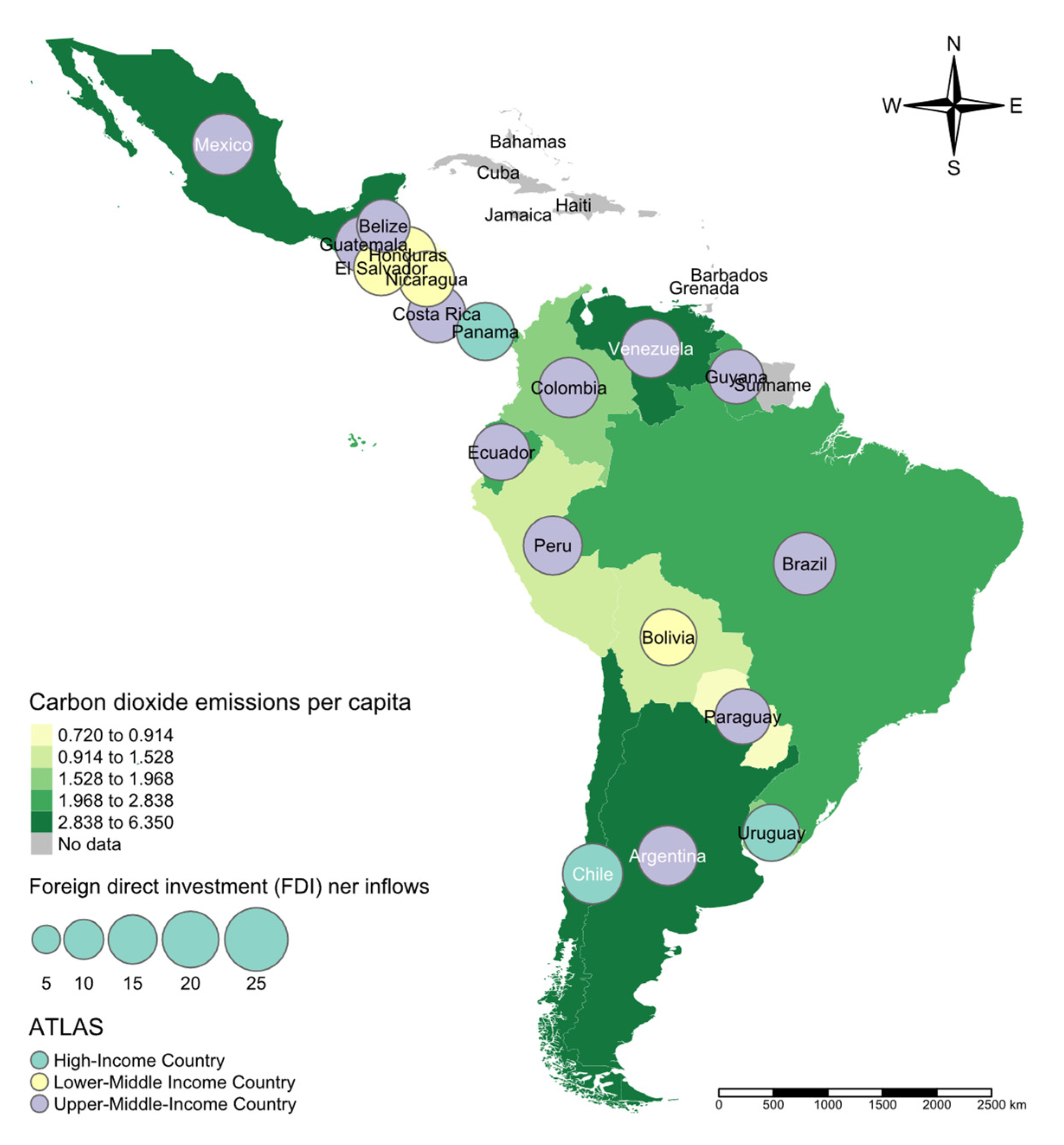
Figure 2 shows the dispersion of the data for the entire sample of Latin American countries according to income level, and Figure 3 shows the map statistics of this data. In the first case, Figure 2 shows that the data between CO₂ emissions and foreign direct investment have a direct relationship at the global level and according to groups of countries by income level. In other words, at higher levels of FDI per capita, higher levels of CO₂ emissions per person are concentrated.

For the 20 countries, the correlation between these two variables is moderate (0.54); however, it is higher in the case of HICs (0.67). For the UMICs (0.40) and LMICs (0.39) groups, the correlation is lower, but in all cases, moderate (a colour is assigned for each country in the sample). An initial analysis of the environmental Kuznets curve (EKC) theory is the functional form of an inverted U.

Figure 2 shows the dispersion of the data for the entire set of Latin American countries and by groups (HICs, UMICs and LMICs). Nevertheless, in none of the cases do the scatter diagrams support this for the EKC; the fits clearly show a positive relationship, the quadratic trend even overlaps the linear, particularly in the UMICs and LMICs.

Likewise, Figure 3 shows the average per capita CO₂ emissions by country and the logarithm of the FDI. In this, it can be observed that countries such as Mexico, Venezuela, Argentina, and Chile concentrate higher levels of CO₂ emissions, as well as FDI inflows at the per capita level.

4. Econometric Strategy

The methodological process consists in five stages. After selecting our estimations between fixed and random effects, and test heteroscedasticity, autocorrelation and contemporary correlation for our panel, we assessed the stationary of the time series, their cointegration (by estimating the cointegration vectors) and finally, we tested the Granger causality. This procedure is explained in stages as follows.

4.1. Estimation Procedure

First, we estimated the fixed and random effects panel models to determine the direction of the relationship between CO₂ emissions per capita (in logarithms) and FDI per capita (in logarithms). Then, we applied the Hausman test [69] to decide between fixed and random effects. In this stage, we applied the modified Wald test [70] to detect heteroscedasticity and tests to detect autocorrelation in the panel and the contemporary correlation, respectively [71,72]. Likewise, recent panel data literature concludes that panel data models are likely to show cross-sectional dependence in the error [73,74]. Our balanced panel data are cross section dependent, as

Table 3. Cross-sectional dependent test.

Group	Variable	CD-Test	p-Value
GLOBAL	CO2 emissions (log)	35.432	0.000
	FDI (log)	26.356	0.000
HICs	CO2 emissions (log)	7.889	0.000
	FDI (log)	7.102	0.000
UMICs	CO2 emissions (log)	15.775	0.000
	FDI (log)	11.291	0.000
LMICs	CO2 emissions (log)	10.092	0.000
	FDI (log)	6.870	0.000

shows.

Findings (cross-section dependence in the panel, as well, autocorrelation, heteroscedasticity, and contemporary correlation in the estimations) suggest the use of estimates with generalized least squares (GLSs) for panel data [60]. Equation (1) expresses the empirical model in the log-log form:

$$\log C{O}_{2 \left(i,t\right)}={\beta }_0+{\beta }_1\log \left(FD{I}_{i,t}\right)+{\epsilon }_{i,t}$$

(1)

4.2. Unit Root Tests

In the second stage, we applied the unit-roots test to identify if the series are stationary (that is if they do not have a trend effect). We used a set of tests that claim that obtaining the first difference eliminates the unit root problem. The tests used comes from Levin, Lin, and Chu (LLC) and Im, Pesaran, and Shin (IPS) respectively [75,76]. Moreover, we apply a simpler non-parametric unit root test called the Fisher type test [77] based on the ADF test [78] and, finally, the Fisher type test based on the Phillips and Perron (PP) test [79]. These four tests can be estimated from the following equation:

$$y_t={\theta }_0+\gamma y_{t-1}+{\delta }_{1}t+{\displaystyle \sum }_{i=2}^p{\sigma }_j{y}_{t-i-1}+{\epsilon }_t$$

(2)

where $y_t$ is the series that is should contain at least the unit root, ${\theta }_0$ is the intersection and ${\delta }_1$ captures the trend effect of time $t$, ${\epsilon }_t$ is the Gaussian error and represents the length of the lag. In Equation (2), when the parameter γ is significant, we can conclude that at least one of the panels has a unit root.

4.3. Cointegration Test

In the third stage, we used cointegration techniques to verify long-term equilibria between the study variables, as well as the existence of a short-term equilibrium [80]. These techniques are based on error correction models (ECVM), globally (for the total panel) and for the different groups of countries, according to income level. We considered the null hypothesis of no cointegration versus cointegration between the variables. It considers structural dynamics rather than residual dynamics. Therefore, we did not put any restrictions on any common factor. Furthermore, the Westerlund [80] error correction model assumes that all variables are integrated in order 1 or I (1) and is written as follows:

$$\Delta x_{it}={\theta }_i{d}_i+{\pi }_i(x_{it-1}-{\beta }_i^{\prime }{y}_{it-1})+{\displaystyle \sum }_{j=1}^m{\pi }_{ij}\Delta x_{it-j}+{\displaystyle \sum }_{j=1}^m{\phi }_{ij}\Delta y_{it-j}+{\epsilon }_{it}$$

(3)

where $d_i=(1-t{)}^{\prime }$ contains the deterministic components and ${\theta }^{\prime }=({\theta }_{1i},{\theta }_{2i}{)}^{\prime }$ is the vector of unknown coefficients to estimate. The error correction coefficient ${\pi }_i$ is estimated using the ordinary least squares method. The above equation can be written as:

$$\Delta x_{it}={\theta }_i{d}_i+{\pi }_i\left(x_{it-1}-{\tau }_i^{\prime }{y}_{it-1}\right)+{\displaystyle \sum }_{j=1}^m{\pi }_{ij}\Delta x_{it-j}+{\displaystyle \sum }_{j=1}^m{\phi }_{ij}\Delta x_{it-j}+{\epsilon }_{it}$$

(4)

where ${\pi }_i$ indicates the speed of adjust the system back to equilibrium. The above equation confirms that the coefficient ${\pi }_i$ is not affected by imposing an arbitrary ${\tau }_i^{\prime }$. We applied the test on the least-squares estimator ${\pi }_i$ and calculated the relation t for each cross-section of countries. These are known as group mean statistics and are written as:

$$G_1=\frac{1}{N}{{\displaystyle \sum }}_{i=1}^N\frac{{\pi }_i}{S.E\left({\widehat{\pi }}_i\right)} \mathrm{and} G_2=\frac{1}{N}{{\displaystyle \sum }}_{i=1}^N\frac{T{\pi }_i}{{\widehat{\pi }}_i\left(1\right)}$$

(5)

where $G_1$ and $G_2$ test the null hypothesis that $H_0:{\pi }_i=0$ for all $i$ against $H_1:{\pi }_i<0$ for some $i$. If the null hypothesis is rejected, then it shows the cointegration relationship of at least one unit of the cross-section. The other two test statistics are presented as:

$$P_1=\frac{{\widehat{\pi }}_i}{S.E\left({\widehat{\pi }}_i\right)} \mathrm{and} P_2=T{\widehat{\pi }}_i$$

(6)

where $P_1$ and $P_2$ test null hypothesis that $H_0:{\pi }_i=0$ for all $i$ against $H_1:{\pi }_i=\pi <0$ for all $i$. The rejection of the null hypothesis implies the rejection of a non-cointegration relationship for the panel of countries as a whole. If there is a cointegration relationship between variables, then this study uses the panel technique to estimate the long- and short-term coefficients.

4.4. Cointegration Vectors

In the fourth stage to estimate the strength of the cointegration vectors [81,82,83,84], we used the dynamic ordinary least squares (DOLSs) model for individual countries and the dynamic ordinary least squares model of panel (PDOLSs), for groups of countries, following the atlas method of the World Bank [13]. The following equation raises the relationship between the two variables:

$$y_{i,t}={\sigma }_i+{\delta }_i{x}_{it}+{\displaystyle \sum }_{j=P}^P{\gamma }_j\Delta x_{i,t-j}+{\mu }_{i,t}$$

(7)

where $y_{i,t}$, are the CO₂ emissions, $i=1, 2, \dots , 20$ countries, $t=1, 2, \dots$, T is the time, $p=1, 2, \dots ,$ $P$ is the number of lags used in the DOLSs regression, while $\partial \log y_{i,t}/\partial \log X_{i,t}={\delta }_i$ measures the change in CO₂ emissions when the variables change explanatory. The coefficients and the value were obtained as the average values in the whole panel using the method of group averages. The PDOLSs estimator is averaged across the dimension between groups and the null hypothesis states that ${\beta }_i={\beta }_0$.

4.5. Granger Causality Test

Finally, following to Dumitrescu and Hurlin [85], we used the Granger’s non-causality approach to account for the problems of heterogeneity in the panel data. The Dumitrescu–Hurlin (DH) test is a modified version of the Granger causality test [86], which is more flexible for $T<N$ and $T>N$ for both unbalanced and heterogeneous data. The DH test uses Equation (6):

$$y_{i,t}={\phi }_i+k{\displaystyle \sum }_{k=1}^k{\gamma }_i^{\left(k\right)}{y}_{it-k}+{\displaystyle \sum }_{k=1}^k{\theta }_i^{\left(k\right)}{x}_{it-k}+{\epsilon }_{it}$$

(8)

where ${\phi }_i$ is the intercept of the shape;${\gamma }_i \mathrm{and} {\theta }_i$ are the slope coefficients; $\epsilon$ is the error term and $k$ is the number of lengths of lag.

5. Results

Table 4. Relation between CO₂ emissions (log) and FDI (log).

	GLOBAL	HICs	UMICs	LMICs
FDI (log)	0.0446 ***	0.0789 ***	0.0274 ***	0.0214 **
	(5.99)	(3.08)	(3.28)	(2.19)
Constant	0.325 ***	0.457 ***	0.506 ***	−0.241 ***
	(7.59)	(2.85)	(9.87)	(−4.35)
Observations	580	87	377	116
Autocorrelation test p-value	0.878	No	0.834	0.921
Fixed effects (time)	No	No	No	No
Fixes effects (country)	No	No	No	No
chi2	35.89	9.490	10.74	4.806
N_g	20	3	13	4

T-statistics in parentheses; ** p < 0.05, and *** p < 0.01 denotes the significance level.

reports the results of the estimated GLS, for the logarithm of CO₂ emissions per capita as a function of the logarithm of FDI, proposed in Equation (1). We estimated that FDI inflows exert a positive and statistically significant effect on CO₂ emissions for the whole panel, where an increase of 1% in FDI inflows increases CO₂ emissions by 0.05%. Likewise, we observed that at the group level, according to the income level, the results are positive and statistically significant in the HICs, UMICs, and LMICs, at different levels of significance. An increase of 1% in FDI inflows increases CO₂ emissions by 0.08%, 0.03%, and 0.02%, respectively, with HICs accounting for the greatest effect on environmental degradation from FDI inflows. These results verify, at the regional level, the PHH hypothesis for developing countries, in which FDI inflows generate a deteriorating effect on the environment. On the other hand, they allow us to reject the EKC hypothesis. However, within the Latin American region by groups of countries, following their per capita income (GNI), we show that there is a lower effect of the FDI on CO₂ emissions in LMICs, which does not necessarily agree with the PHH hypothesis.

Next, using unit root tests for the panel data, we verified whether the series are stationary. To ensure the robustness of the results, we used four tests, those of [72,75], which are known respectively in the empirical literature on panel data as the LLC and IPS. The results obtained from these tests were compared with those of [76], who proposed using a simpler non-parametric unit root test called the Fisher-type test and based on the ADF test [77] and the test Fisher type based on the P&P test [78], based on what is stated in Equation (2). The tests were applied with and without the effects of time.

The results shown in

Table 5. Unit root test in first differences.

		Without the Effect of Time				With the Effect of Time
Groups	Variable	PP	ADF	LLC	IPS	PP	ADF	LLC	IPS
GLOBAL	CO2pci,t	−23.64 ***	−9.06 ***	−21.24 ***	−21.88 ***	−22.64 ***	−8.67 ***	−15.33 ***	−18.54 ***
	FDIpci,t	−28.10 ***	−11.49 ***	−24.56 ***	−24.48 ***	−26.49 ***	−9.71 ***	−15.75 ***	−20.15 ***
HICs	CO2pci,t	−8.76 ***	−4.78 ***	-4.83 ***	−6.61 ***	−7.76 ***	−3.69 ***	−3.79 ***	−5.71 ***
	FDIpci,t	−10.66 ***	−3.06 ***	−7.28 ***	−8.41 ***	−10.52 ***	−3.24 ***	−7.05 ***	−8.78 ***
UMICs	CO2pci,t	−18.44 ***	−7.66 ***	−17.52 ***	−17.92 ***	−17.14 ***	−6.49 ***	−14.30 ***	15.61 ***
	FDIpci,t	−23.04 ***	−13.84 ***	−15.79 ***	−17.66 ***	−21.46 ***	−8.41 ***	−13.73 ***	−16.38 ***
LMICs	CO2pci,t	−12.03 ***	−2.32 **	−11.47 ***	−10.91 ***	−13.01 ***	−4.50 ***	−4.92 ***	−8.39 ***
	FDIpci,t	−12.05 ***	−4.02 ***	−18.01 ***	−15.68 ***	−11.43 ***	−3.77 ***	−4.42 ***	−7.91 ***

Note: ** p < 0.05, and *** p < 0.01 denotes the significance level.

are evidence that the series have an order of integration I (1). All the tests ensure that the series used in subsequent estimates do not have the unit root problem. In the next stage of this investigation, we verified the existence of cointegration vectors in the long and short term between the variables.

In the next stage, we used ECVM developed by Westerlund [79] for the panel data to determine the short-term equilibrium, according to what was stated in Equations (3) and (4). The existence of a short-term equilibrium implies that a change in foreign direct investment rapidly translates into changes in per capita CO₂ emissions.

Westerlund suggested the bootstrap approach, which makes the inference possible even under very general forms of cross-sectional dependence. From that, our results reported in

Table 6. Results of the Westerlund ECVM error correction model.

Group	Stat.	Value	Z-Value	p-Value	Robust p-Value
Global	Gτ	−2.88	−2.89	0.002	0.270
	Gα	−14.78	−1.938	0.026	0.610
	Pτ	−12.68	−3.761	0.000	0.110
	Pα	−13.88	−3.690	0.000	0.270
HICs	Gτ	−3.43	−2.32	0.010	0.180
	Gα	−23.26	−2.96	0.002	0.050
	Pτ	−5.91	−2.63	0.004	0.120
	Pα	−21.14	−3.53	0.000	0.080
UMICs	Gτ	−2.90	−2.42	0.008	0.290
	Gα	−13.35	−0.80	0.215	0.760
	Pτ	−10.28	−3.10	0.001	0.150
	Pα	−12.68	−2.25	0.012	0.430
LMICs	Gτ	−2.39	−0.09	0.446	0.710
	Gα	−13.06	−0.35	0.363	0.690
	Pτ	−4.58	−0.41	0.342	0.660
	Pα	−11.91	−0.99	0.161	0.620

discard the existence of a short-term equilibrium, for the whole panel and for each of the groups of countries that we are considering.

To determine the existence of the long-term equilibrium, from Equation (5) we used the heterogeneous panel cointegration test developed by Pedroni [81], which allows incorporating cross-sectional interdependence with different individual effects. This analytical framework allows cointegration tests on both heterogeneous and homogeneous panels, incorporating seven repressors based on seven residue-based statistics. Of these seven tests, the panel υ-statistic is a one-sided test in which high positive values reject the null hypothesis of no cointegration. While, for the rest of the statistics, high negative values reject the null hypothesis.

Table 7. Pedroni cointegration test.

	GLOBAL	HICs	UMICs	LMICs
Within dimension test statistics
Panel υ-statistic	0.44	1.25	−0.04	0.72
Panel p-statistic	−1.83 *	−4.10 ***	−0.88	−2.20 **
Panel PP-statistic	−2.46 **	−4.07 ***	−1.39	−2.27 **
Panel ADF statistic	−0.33	−3.03 ***	−0.95	−1.51
Between dimension test statistics
Group p-statistic	−0.77	−3.11 ***	−0.07	−1.19
Group PP-statistic	−2.01 **	−4.42 ***	−0.95	−1.95 *
Group ADF statistic	0.13	−1.73 *	1.58	−0.36

Note: * p < 0.10, ** p < 0.05, and *** p < 0.01 denotes the significance level.

reports the statistics within and between dimensions. These results are ambiguous because of the heterogeneity of the panel. For LMICs (as for the entire panel), the panel ρ and PP statistic suggest the existence of cointegration between the CO₂ emissions and FDI series (similar to the group PP statistic), but the evidence of the panel υ and ADF statistic do not allow us to reject the null hypothesis of non-cointegration. For the HICs the majority of statistics within and between dimensions led us to reject the null and therefore, our results indicate that CO₂ emissions per capita and foreign direct investment have a joint and simultaneous movement during the period of 1990–2018 in high income countries. The latter is opposite for upper-middle-income countries.

Table 8. Results of the DOLSs panel.

HIC			UMICs			LIMCs
Country	FDI (β)	t-Statistic	Country	FDI (β)	t-Statistic	Country	FDI (β)	t-Statistic
Chile	0.315 ***	3.849	Argentina	0.019	0.511	Bolivia	−0.060	−1.102
Panama	0.223 ***	3.186	Belize	−0.002	−0.012	Nicaragua	−0.082	−0.758
Uruguay	0.076 ***	4.056	Brazil	0.143 **	2.250	El Salvador	0.047	1.180
			Colombia	0.112	0.486	Honduras	0.234 ***	7.164
			Costa Rica	0.174	1.542
			Dominican Republic	−0.209	−1.671 *
			Ecuador	−0.064	−1.899 *
			Guatemala	0.008	0.054
			Guyana	−0.064	−1.321
			Mexico	0.293 ***	5.265
			Paraguay	0.142 ***	9.699
			Peru	0.626 ***	6.416
			Venezuela	0.114 ***	6.301

Note: * p < 0.10, ** p < 0.05, and *** p < 0.01 denotes the significance level.

reports the results of the DOLSs model by country. Our findings reveal that a 1% increase in FDI per capita is associated with an increase in CO₂ emissions per capita of 0.315%, 0.223%, and 0.076% for Chile, Panama, and Uruguay, respectively, which are all the higher income countries in the Latin American region. These results go in line with the outcome of Table 7. For upper-middle-income countries (65% of the panel), the results are mixed. For Brazil, Mexico, Paraguay, Peru, and Venezuela, 1% of increase in FDI per capita is associated with an increase in CO₂ emissions per capita of 0.143%, 0.293%, 0.142%, 0.626%, and 0.114%, respectively. However, in Dominican Republic and Ecuador, a 1% increase in FDI per capita is associated with a decrease in CO₂ emissions per capita of 0.209% and 0.064%, respectively. Finally, for LMICs, we only can reject the null of non-cointegration in Honduras, with a positive (0.234) weak cointegration vector (very far from 1). All statistically significant vectors are weak, except that from Peru.

To obtain the strength of the cointegration vector by groups of countries,

Table 9. Results of the PDOLSs panel test per country group.

	With Time Dummy		Without Time Dummy
Groups	PDOLSs	t-Stat	PDOLSs	t-Stat
GLOBAL	0.103 ***	10.110	0.127 ***	20.650
HICs	−0.014	0.956	0.223 ***	16.240
UMICs	0.074 ***	5.688	0.111 ***	9.116
LMICs	−0.011 **	−2.035	0.106 ***	15.670

Note: ** p < 0.05, and *** p < 0.01 denotes the significance level.

shows the results of the PDOLSs estimates with and without time variables. The estimators ${\beta }_i$ of the different income levels are not close to 1. Nevertheless, in most of the cases (except for HICs, with a time dummy), we found evidence of a weak cointegration between the CO₂ emissions per capita and FDI per capita.

Finally, from Equation (6), we determined the Granger-type causality (

Table 10. Causality tests following Dumitrescu–Hurlin (2012).

Causal Direction	Group	W-Bar	Z-Bar	p-Value	Z-Bar Tilde	p-Value
ΔFDIpc → ΔCO2pc	GLOBAL	1.93	−0.15	0.897	−0.51	0.629
	HICs	0.45	−1.34	0.170	−1.24	0.124
	UMICs	1.71	−0.52	0.651	−0.74	0.457
	LMICs	3.77	1.77	0.100	1.27	0.139
ΔCO2pc → ΔFDIpc	GLOBAL	1.39	−1.36	0.268	−1.49	0.128
	HICs	1.05	−0.82	0.450	−0.82	0.372
	UMICs	1.37	−1.14	0.331	−1.23	0.214
	LMIC	1.72	−0.28	0.801	−0.40	0.678

) of the variables from the formalization developed by Dumitrescu and Hurlin [85]. Because of the evidence of cross-section dependence, we developed a bootstrap approach suggested by Dumitrescu and Hurlin [85]. We determined that there are no causal relationships between CO₂ emissions per capita and foreign direct investment, globally and by the group of countries.

6. Discussion of Results

The economic literature presented ambiguous results regarding the effects that FDI flows can generate environmental degradation, even if we analyse these effects by groups of countries (developed or developing) [8]. Our findings for 20 Latin American countries in the period of 1990–2018 agree with the PHH that suggests that, in developing countries, such as Latin American, the effect of FDI is positive on environmental degradation, due to polluting multinational corporations directing their investments to countries with weaker environmental regulations [87,88,89]. These results are contradictory to those expressed by the EKC hypothesis, which in contrast, suggest a quadratic relationship (as an inverted U shape) between the variables [90]. These results coincide with extensive empirical evidence [14,15,28,55,57], for developing countries such as some of the Asian, African [22,24] and European countries, such as Turkey and France [54,56], and Mediterranean countries [91]. The study by Chang [34], for 65 countries, also shows that increases in FDI can increase CO₂ emissions when the degree of corruption is relatively high. In fact, if the FDI is sourced from developing countries it would be detrimental to the environmental environment of low- and lower-middle-income host countries [41].

Within the region (Latin America), our findings estimated with generalized least squares (GLSs) are supported by [21,46]. However, for this region of analysis, there are other works such as that of [19,20], who reject the PHH. It should be noted that, within Latin American countries, under the hypothesis of pollution havens, those that are in the LMICs were expected to be those where the FDI has the greatest impact on CO₂ emissions. However, the results show that the greatest impact is evidenced in those economies who are HIC. Similarly, the results shown in the CD tests coincide with those found by [92,93]. In a global context, the results showed the existence of interactions between countries caused by investment flows, political integration agreements, etc.

The results presented in this article reject the existence of a short-term equilibrium, based on the error correction model (ECVM) developed by Westerlund [80]. In contrast, we found some evidence that support a long-term equilibrium between the series; except for UMICs that contribute 65% of the panel, as Table 8 and Table 9 show. The short-term results contrast with findings of [52,53]. However, the long-term cointegration results in this research are in line with those of [28], for South and Southeast Asia [52,53]. This supports the point of [88], where regardless of the level of development, there is a heterogeneous influence of the FDI.

From causality tests [85], our results contradict the conclusions of [26,54,55,94,95]. These authors reveal a unidirectional causality of the FDI to CO₂ emissions. However, our findings agree with those of [44] that show no causality, in any way, between the study variables. In that sense, despite the results of estimations in Table 4, we cannot conclude that FDI is the cause of the increase in CO₂ emissions in Latin American countries, nor the other way around.

7. Conclusions

The main objective of this study was to test the EKC and PHH hypotheses, for which the relationship between CO₂ emissions and FDI is analysed in various contexts. This article offers empirical evidence in the context of 20 Latin American economies, characterised by developing countries, and tests the relationship between CO₂ emissions and FDI over a period from 1990 to 2018. In addition, the sample of countries was classified into three subsamples (HICs, UMICs and LMICs) according to the atlas method of the World Bank [13]. For the analyses, econometric techniques are used. Firstly, it was applied in the CD test, to determine the existence of independence between transversal units. Followed by unit root tests (PP, ADF, LLC, IPS) to determine the stationarity of the set of variables, and then two cointegration tests were applied to determine the equilibrium relationships both in the short and long term. In addition, a Granger causality test was used to observe the causal links between the variables.

The results of the estimations, in a general way allow us to identify a direct relationship between CO₂ emissions and FDI, but they do not show a quadratic relationship and therefore, it is concluded in a rejection of the hypothesis of the environmental Kuznets curve (EKC). On the other hand, in developing countries, these results are related to the PHH, which establishes that highly polluting multinational companies move to developing countries with weaker environmental standards. However, the estimates formed by groups of countries offer unexpected information according to the PHH hypothesis, since the impact of FDI on CO₂ emissions is similar for lower-middle-income countries (LMICs) and upper-middle-income countries (UMICs), but it is about three times higher for high-income countries (HICs). This represents an inconsistency in the Latin American context, since the impact that we expected has a higher coefficient for the economies with lower-middle incomes (UMICs and LMICs).

The results of this article did not present causal relationships in any direction between the variables studied, nor any of the subsamples by income level. On the other hand, they only showed some evidence of a long-term equilibrium. There is no evidence of a short-term equilibrium.

Finally, the evidence demonstrated in this article might contribute with certain policy implications, such as establishing strategies to mitigate the environmental impact caused by the FDI. However, in developing countries, sustainable issues, many of them supported by the results of the EKC, have been interpreted by some policymakers as conveying a message about priorities [96]. The question in this study is which comes first, FDI flows or cleaning up the environment? Certainly, each developing economy tends to prioritize, in the short term, the solution of “immediate” problems such as economic growth, that can be driven by foreign direct investment flows (although the literature is ambiguous in this regard, see for example, the literature review in Alvarado et al. [97]. Then, in the long term, economies worry about environmental damage, as a “non-immediate” problem. This means that when thinking about a sustainable economy, responsible with future generations, caring for the environment is in the background (“the second-best theory”). In Latin American, following our results, there is no evidence that in the long term the relationship of the variables behaves similar to the environmental Kuznets curve, especially in the case of countries with a high-income, according to the atlas method of the World Bank [13]. In fact, we have some evidence that the effects of the FDI per capita on CO₂ emissions have a positive long-term equilibrium, except in UMICs such as the Dominican Republic and Ecuador. In this context, Latin American countries must design strategies that attract an environmentally friendly FDI that, despite having a negative impact (direct effect on CO₂ emissions) in the short term (due to the urgent priorities of developing economies), guarantee in the long term (“the second-best theory”) a reduction in environmental pollution and, therefore, the applicability of the EKC. In other words, the region must address policies that generate the inverted U when we refer to the relationship between the CO₂ emissions and FDI.

This study has minor limitations. For example, new research presents a challenge by not confirming EKC or PHH in its estimates. Therefore, future research can expand the sample size or broaden the analysis between regions. In addition, the origin of the FDI can be identified according to the level of development of the investing economies, which can produce interesting inferences in the context of the Latin America region.

References

1. Kuznets, S. Economic Growth and Income Inequality. Am. Econ. Rev. 1955, 45, 1–28. [Google Scholar]
2. Kuznets, S. Quantitative aspects of the economic growth of nations: Viii. distribution of income by size. Econ. Dev. Cul. Chang. 1963, 11, 1–92. [Google Scholar] [CrossRef] [Green Version]
3. Stern, D.; Common, M.; Barbier, E. Economic growth and environmental degradation: The environmental Kuznets curve and sustainable development. World Dev. 1996, 204, 1151–1160. [Google Scholar] [CrossRef]
4. Birdsall, N.; Wheeler, D. Trade policy and industrial pollution in Latin America: Where are the pollution havens? J. Environ. Dev. 1993, 2, 137–149. [Google Scholar] [CrossRef]
5. Copeland, B.; Taylor, S. North-South trade and the environment. Q. J. Econ. 1994, 109, 755–787. [Google Scholar] [CrossRef]
6. Bakhsh, K.; Rose, S.; Ali, M.F.; Ahmad, N.; Shahbaz, M. Economic growth, CO2 emissions, renewable waste and FDI relation in Pakistan: New evidences from 3SLS. J. Environ. Manag. 2017, 196, 627–632. [Google Scholar] [CrossRef]
7. Shahbaz, M.; Haouas, I.; Van Hoang, T.H. Economic growth and environmental degradation in Vietnam: Is the environmental Kuznets curve a complete picture? Emerg. Mark. Rev. 2019, 38, 197–218. [Google Scholar] [CrossRef]
8. Demena, B.A.; Afesorgbor, S.K. The effect of FDI on environmental emissions: Evidence from a meta-analysis. Energy Policy 2020, 138, 111192. [Google Scholar] [CrossRef]
9. Neequaye, N.A.; Oladi, R. Environment, growth, and FDI revisited. Int. Rev. Econ. Financ. 2015, 39, 47–56. [Google Scholar] [CrossRef]
10. Shahbaz, M.; Nasreen, S.; Abbas, F.; Anis, O. Does foreign direct investment impede environmental quality in high-, middle-, and low-income countries? Energy Econ. 2015, 51, 275–287. [Google Scholar] [CrossRef]
11. Paramati, S.R.; Ummalla, M.; Apergis, N. The effect of foreign direct investment and stock market growth on clean energy use across a panel of emerging market economies. Energy Econ. 2016, 56, 29–41. [Google Scholar] [CrossRef]
12. Solarin, S.A.; Al-Mulali, U. Influence of foreign direct investment on indicators of environmental degradation. Environ. Sci. Pollut. 2018, 25, 24845–24859. [Google Scholar] [CrossRef] [PubMed]
13. World Bank. World Bank Country and Lending Groups. Washington D.C. Available online: https://bit.ly/3i7FKeJ (accessed on 22 December 2019).
14. Sabir, S.; Gorus, M.S. The impact of globalization on ecological footprint: Empirical evidence from the South Asian countries. Environ. Sci. Pollut. 2019, 26, 33387–33398. [Google Scholar] [CrossRef] [PubMed]
15. Hanif, I.; Faraz-Raza, S.M.; Gago-de-Santos, P.; Abbas, Q. Fossil fuels, foreign direct investment, and economic growth have triggered CO2 emissions in emerging Asian economies: Some empirical evidence. Energy 2019, 171, 493–501. [Google Scholar] [CrossRef]
16. Ali, M.U.; Gong, Z.; Ali, M.U.; Wu, X.; Yao, C. Fossil energy consumption, economic development, inward FDI impact on CO2 emissions in Pakistan: Testing EKC hypothesis through ARDL model. Int. J. Financ. Econ. 2021, 26, 3210–3221. [Google Scholar] [CrossRef]
17. To, A.H.; Ha, D.T.T.; Nguyen, H.M.; Vo, D.H. The impact of foreign direct investment on environment degradation: Evidence from emerging markets in Asia. Int. J. Environ. Res. 2019, 16, 1636. [Google Scholar] [CrossRef] [Green Version]
18. Muhammad, B.; Khan, S. Effect of bilateral FDI, energy consumption, CO2 emission and capital on economic growth of Asia countries. Energy Rep. 2019, 5, 1305–1315. [Google Scholar] [CrossRef]
19. Albulescu, C.T.; Tiwari, A.K.; Yoon, S.M.; Kang, S.H. FDI, income, and environmental pollution in Latin America: Replication and extension using panel quantiles regression analysis. Energy Econ. 2019, 84, 104504. [Google Scholar] [CrossRef]
20. Cansino, J.; Román-Collado, R.; Molina, J. Quality of institutions, technological progress, and pollution havens in Latin America. An analysis of the environmental Kuznets curve hypothesis. Sustainability 2019, 11, 3708. [Google Scholar] [CrossRef] [Green Version]
21. Sapkota, P.; Bastola, U. Foreign direct investment, income, and environmental pollution in developing countries: Panel data analysis of Latin America. Energy Econ. 2017, 64, 206–212. [Google Scholar] [CrossRef]
22. Abdouli, M.; Hammami, S. The impact of FDI inflows and environmental quality on economic growth: An empirical study for the MENA countries. J. Knowl. Econ. 2017, 8, 254–278. [Google Scholar] [CrossRef] [Green Version]
23. Gorus, M.S.; Aslan, M. Impacts of economic indicators on environmental degradation: Evidence from MENA countries. Renew. Sustain. Energ. Rev. 2019, 103, 259–268. [Google Scholar] [CrossRef]
24. Bokpin, G. Foreign direct investment and environmental sustainability in Africa: The role of institutions and governance. Res. Int. Bus. Financ. 2017, 39, 239–247. [Google Scholar] [CrossRef]
25. Shahbaz, M.; Balsalobre-Lorente, D.; Sinha, A. Foreign direct Investment–CO2 emissions nexus in Middle East and North African countries: Importance of biomass energy consumption. J. Clean. Prod. 2019, 217, 603–614. [Google Scholar] [CrossRef] [Green Version]
26. Abdouli, M.; Hammami, S. The dynamic links between environmental quality, foreign direct investment, and economic growth in the middle eastern and North African countries (MENA region). J. Knowl. Econ. 2018, 9, 833–853. [Google Scholar] [CrossRef]
27. Kivyiro, P.; Arminen, H. Carbon dioxide emissions, energy consumption, economic growth, and foreign direct investment: Causality analysis for Sub-Saharan Africa. Energy 2014, 74, 595–606. [Google Scholar] [CrossRef]
28. Behera, S.R.; Dash, D.P. The effect of urbanization, energy consumption, and foreign direct investment on the carbon dioxide emission in the SSEA (South and Southeast Asian) region. Renew. Sustain. Energ. Rev. 2017, 70, 96–106. [Google Scholar] [CrossRef]
29. Halliru, A.M.; Loganathan, N.; Golam Hassan, A.A. Does FDI and economic growth harm environment? Evidence from selected West African countries. Transnatl. Corp. 2020, 13, 237–251. [Google Scholar]
30. Pazienza, P. The relationship between CO2 and foreign direct investment in the agriculture and fishing sector of OECD countries: Evidence and policy considerations. Intellect. Econ. 2015, 9, 55–66. [Google Scholar] [CrossRef]
31. De Pascale, G.; Sardaro, R.; Faccilongo, N.; Contò, F. What is the influence of FDI and international people flows on environment and growth in OECD countries? A panel study. Environ. Impact Assess. Rev. 2020, 84, 106434. [Google Scholar] [CrossRef]
32. Pazienza, P. The impact of FDI in the OECD manufacturing sector on CO2 emission: Evidence and policy issues. Environ. Impact Assess. Rev. 2019, 77, 60–68. [Google Scholar] [CrossRef]
33. Ahmed, Z.; Zafar, M.W.; Ali, S.; Kahn, D. Linking urbanization, human capital, and the ecological footprint in G7 countries: An empirical analysis. Sustain. Cities Soc. 2020, 55, 102064. [Google Scholar] [CrossRef]
34. Chang, S.C. Threshold effect of foreign direct investment on environmental degradation. Port. Econ. J. 2015, 14, 75–102. [Google Scholar] [CrossRef] [Green Version]
35. Saud, S.; Chen, S.; Haseeb, A.; Sumayya, A. The role of financial development and globalization in the environment: Accounting ecological footprint indicators for selected one-belt-one-road initiative countries. J. Clean. Prod. 2020, 250, 119518. [Google Scholar] [CrossRef]
36. Du, X.; Xie, Z. Occurrence of turning point on environmental Kuznets curve in the process of (de)industrialization. Struct. Chang. Econ. Dyn. 2019, 53, 359–369. [Google Scholar] [CrossRef]
37. Chandran, V.G.R.; Tang, C.F. The impacts of transport energy consumption, foreign direct investment and income on CO2 emissions in ASEAN-5 economies. Renew. Sustain. Energ. Rev. 2013, 24, 445–453. [Google Scholar] [CrossRef]
38. Guzel, A.E.; Okumus, İ. Revisiting the pollution haven hypothesis in ASEAN-5 countries: New insights from panel data analysis. Environ. Sci. Pollut. 2020, 27, 18157–18167. [Google Scholar] [CrossRef] [PubMed]
39. Xiong, S.Y.; Hussain, J. The implication of technological innovation and tourism development on FDI-growth-environment nexus in association of Southeast Asian countries: A simultaneity modeling analysis. Energy Sources B Econ. Plan. Policy. 2021, 16, 878–902. [Google Scholar]
40. Abdouli, M.; Kamoun, O.; Hamdi, B. The impact of economic growth, population density, and FDI inflows on CO2 emissions in BRICTS countries: Does the Kuznets curve exist? Empir. Econ. 2018, 54, 1717–1742. [Google Scholar] [CrossRef]
41. Adeel-Farooq, R.M.; Riaz, M.F.; Ali, T. Improving the environment begins at home: Revisiting the links between FDI and environment. Energy 2021, 215, 119150. [Google Scholar] [CrossRef]
42. Udemba, E.N.; Yalçıntaş, S. Interacting force of foreign direct invest (FDI), natural resource and economic growth in determining environmental performance: A nonlinear autoregressive distributed lag (NARDL) approach. Resour. Policy 2021, 73, 102168. [Google Scholar] [CrossRef]
43. Kisswani, K.M.; Zaitouni, M. Does FDI affect environmental degradation? Examining pollution haven and pollution halo hypotheses using ARDL modelling. J. Asian Pac. Econ. 2021, 1–27. [Google Scholar] [CrossRef]
44. Hassan, S.A.; Nosheen, M. Estimating the Railways Kuznets Curve for high income nations—A GMM approach for three pollution indicators. Energy Rep. 2019, 5, 170–186. [Google Scholar] [CrossRef]
45. Sarkodie, S.A.; Strezov, V. Effect of foreign direct investments, economic development and energy consumption on greenhouse gas emissions in developing countries. Sci. Total Environ. 2019, 646, 862–871. [Google Scholar] [CrossRef]
46. Dhrifi, A.; Jaziri, R.; Alnahdi, S. Does foreign direct investment and environmental degradation matter for poverty? Evidence from developing countries. Struct. Chang. Econ. Dyn. 2020, 52, 13–21. [Google Scholar] [CrossRef]
47. Essandoh, O.K.; Islam, M.; Kakinaka, M. Linking international trade and foreign direct investment to CO2 emissions: Any differences between developed and developing countries? Sci. Total Environ. 2020, 712, 136437. [Google Scholar] [CrossRef] [PubMed]
48. Xie, Q.; Sun, Q. Assessing the impact of FDI on PM2.5 concentrations: A nonlinear panel data analysis for emerging economies. Environ. Impact Assess. Rev. 2020, 80, 106314. [Google Scholar] [CrossRef]
49. Muhammad, S.; Long, X.; Salman, M.; Dauda, L. Effect of urbanization and international trade on CO2 emissions across 65 belt and road initiative countries. Energy 2020, 196, 117102. [Google Scholar] [CrossRef]
50. Bildirici, M.; Gokmenoglu, S.M. The impact of terrorism and FDI on environmental pollution: Evidence from Afghanistan, Iraq, Nigeria, Pakistan, Philippines, Syria, Somalia, Thailand and Yemen. Environ. Impact Assess. Rev. 2020, 81, 106340. [Google Scholar] [CrossRef]
51. Zafar, M.W.; Zaidi, S.A.H.; Khan, N.R.; Mirza, F.M.; Hou, F.; Kirmanis, A.A. The impact of natural resources, human capital, and foreign direct investment on the ecological footprint: The case of the United States. Resour. Policy 2019, 63, 101428. [Google Scholar] [CrossRef]
52. Haug, A.A.; Ucal, M. The role of trade and FDI for CO2 emissions in Turkey: Nonlinear relationships. Energy Econ. 2019, 81, 297–307. [Google Scholar] [CrossRef]
53. Koçak, E.; Şarkgüneşi, A. The impact of foreign direct investment on CO2 emissions in Turkey: New evidence from cointegration and bootstrap causality analysis. Environ. Sci. Pollut. 2018, 25, 790–804. [Google Scholar] [CrossRef] [PubMed]
54. Balibey, M. Relationships among CO2 Emissions, Economic growth and foreign direct investment and the environmental Kuznets curve hypothesis in Turkey. Int. J. Energy Econ. Policy 2015, 5, 1042–1049. [Google Scholar]
55. Lau, L.S.; Choong, C.K.; Eng, Y.K. Investigation of the environmental Kuznets curve for carbon emissions in Malaysia: DO foreign direct investment and trade matter? Energy Policy 2014, 68, 490–497. [Google Scholar] [CrossRef]
56. Shahbaz, M.; Nasir, M.; Roubaud, D. Environmental degradation in France: The effects of FDI, financial development, and energy innovations. Energy Econ. 2018, 74, 843–857. [Google Scholar] [CrossRef] [Green Version]
57. Minh, N. Foreign Direct Investment and Carbon Dioxide Emissions: Evidence from Capital of Vietnam. Int. J. Energy Econ. Policy 2020, 10, 76–83. [Google Scholar] [CrossRef]
58. Phuong, N.; Tuyen, L. The relationship between foreign direct investment, economic growth and environmental pollution in Vietnam: An autoregressive distributed lags approach. Int. J. Energy Econ. Policy 2018, 8, 138–145. [Google Scholar]
59. Ridzuan, A.; Ismail, N.; Hamat, A. Does foreign direct investment successfully lead to sustainable development in Singapore? Economies 2017, 5, 29. [Google Scholar] [CrossRef] [Green Version]
60. Hille, E.; Shahbaz, M.; Moosa, I. The impact of FDI on regional air pollution in the Republic of Korea: A way ahead to achieve the green growth strategy? Energy Econ. 2019, 81, 308–326. [Google Scholar] [CrossRef] [Green Version]
61. Liu, Q.; Wang, S.; Zhang, W.; Zhan, D.; Li, J. Does foreign direct investment affect environmental pollution in China’s cities? A spatial econometric perspective. Sci. Total Environ. 2018, 613, 521–529. [Google Scholar] [CrossRef]
62. Zhu, L.; Hao, Y.; Lu, Z.N.; Wu, H.; Ran, Q. Do economic activities cause air pollution? Evidence from China’s major cities. Sustain. Cities Soc. 2019, 49, 101593. [Google Scholar] [CrossRef]
63. Liu, J.; Qu, J.; Zhao, K. Is China’s development conforms to the environmental Kuznets curve hypothesis and the pollution haven hypothesis? J. Clean. Prod. 2019, 234, 787–796. [Google Scholar] [CrossRef]
64. Long, R.; Gan, X.; Chen, H.; Wang, J.; Li, Q. Spatial econometric analysis of foreign direct investment and carbon productivity in China: Two-tier moderating roles of industrialization development. Resour. Conserv. Recycl. 2020, 155, 104677. [Google Scholar] [CrossRef]
65. Xu, S.C.; Li, Y.W.; Miao, Y.M.; Gao, C.; He, Z.X.; Shen, W.X.; Wang, S.X. Regional differences in nonlinear impacts of economic growth, export and FDI on air pollutants in China based on provincial panel data. J. Clean. Prod. 2019, 228, 455–466. [Google Scholar] [CrossRef]
66. An, T.; Xu, C.; Liao, X. The impact of FDI on environmental pollution in China: Evidence from spatial panel data. Environ. Sci. Pollut. 2021, 28, 44085–44097. [Google Scholar] [CrossRef]
67. Zameer, H.; Yasmeen, H.; Zafar, M.W.; Waheed, A.; Sinha, A. Analyzing the association between innovation, economic growth, and environment: Divulging the importance of FDI and trade openness in India. Environ. Sci. Pollut. 2020, 27, 29539–29553. [Google Scholar] [CrossRef]
68. World Bank. World Development Indicators. Washington D.C. Available online: https://bit.ly/3lUF6SR (accessed on 23 January 2020).
69. Hausman, J.A. Specification tests in econometrics. Econometrica 1978, 46, 1251. [Google Scholar] [CrossRef] [Green Version]
70. Wooldridge, J. Econometric Analysis of Cross Section and Panel Data, 2nd ed.; The MIT Press Cambridge: London, UK, 2002. [Google Scholar]
71. Wooldridge, J.M. On the application of robust, regression- based diagnostics to models of conditional means and conditional variances. J. Econom. 1991, 47, 5–46. [Google Scholar] [CrossRef]
72. Breusch, T.S.; Pagan, A.R. The Lagrange multiplier test and its applications to model specification in econometrics. Rev. Econ. Stud. 1980, 47, 239–253. [Google Scholar] [CrossRef]
73. Pesaran, M. General Diagnostic Tests for Cross Section Dependence in Panels; Working Paper; IZA Bonn: Bonn, Germany, 2004. [Google Scholar]
74. Pesaran, M. Testing weak cross-sectional dependence in large panels. Econom. Rev. 2015, 34, 1089–1117. [Google Scholar] [CrossRef] [Green Version]
75. Levin, A.; Lin, C.F.; James Chu, C.S. Unit root tests in panel data: Asymptotic and finite-sample properties. J. Econom. 2002, 108, 1–24. [Google Scholar] [CrossRef]
76. Im, K.S.; Pesaran, M.H.; Shin, Y. Testing for unit roots in heterogeneous panels. J. Econom. 2003, 115, 53–74. [Google Scholar] [CrossRef]
77. Maddala, G.S.; Wu, S. A comparative study of unit root tests with panel data and a new simple test. Oxf. Bull. Econ. Stat. 1999, 61, 631–652. [Google Scholar] [CrossRef]
78. Dickey, D.A.; Fuller, W.A. Likelihood ratio statistics for autoregressive time series with a unit root. Econometrica 1981, 49, 1057. [Google Scholar] [CrossRef]
79. Phillips, P.C.B.; Perron, P. Testing for a unit root in time series regression. Biometrika 1988, 75, 335–346. [Google Scholar] [CrossRef]
80. Westerlund, J. Testing for error correction in panel data. Oxf. Bull. Econ. Stat. 2007, 69, 709–748. [Google Scholar] [CrossRef] [Green Version]
81. Pedroni, P. Critical values for cointegration tests in heterogeneous panels with multiple regressors. Oxf. Bull. Econ. Stat. 1999, 61, 653–670. [Google Scholar] [CrossRef]
82. Pedroni, P. Purchasing power parity tests in cointegrated panels. Rev. Econ. Stat. 2001, 83, 727–731. [Google Scholar] [CrossRef] [Green Version]
83. Pedroni, P. Panel Cointegration: Asymptotic and Finite Sample Properties of Pooled Time Series Tests with an Application to the PPP Hypothesis. Econom. Theory 2004, 20, 597–625. [Google Scholar] [CrossRef] [Green Version]
84. Neal, T. Panel Cointegration Analysis with Xtpedroni. Stata J. 2014, 14, 684–692. [Google Scholar] [CrossRef] [Green Version]
85. Dumitrescu, E.I.; Hurlin, C. Testing for Granger non-causality in heterogeneous panels. Econ. Model. 2012, 29, 1450–1460. [Google Scholar] [CrossRef] [Green Version]
86. Granger, C.W.J. Investigating causal relations by econometric models and cross-spectral methods. Econometrica 1969, 37, 424–438. [Google Scholar] [CrossRef]
87. Wang, C.; Jiayu, C. Analyzing on the impact mechanism of foreign direct investment (FDI) to energy consumption. Energy Procedia 2019, 159, 515–520. [Google Scholar] [CrossRef]
88. Ahmad, M.; Jabeen, G.; Wu, Y. Heterogeneity of pollution haven/halo hypothesis and environmental Kuznets curve hypothesis across development levels of Chinese provinces. J. Clean. Prod. 2021, 285, 124898. [Google Scholar] [CrossRef]
89. Sabir, S.; Qayyum, U.; Majeed, T. FDI and environmental degradation: The role of political institutions in South Asian countries. Environ. Sci. Pollut. Res. 2020, 27, 32544–32553. [Google Scholar] [CrossRef]
90. Adamu, T.; Haq, I.; Shafiq, M. Analyzing the impact of energy, export variety, and FDI on environmental degradation in the context of environmental Kuznets curve hypothesis: A case study of India. Energies 2019, 12, 1076. [Google Scholar] [CrossRef] [Green Version]
91. Gyamfi, B.A.; Adebayo, T.S.; Bekun, F.V.; Agyekum, E.B.; Kumar, N.M.; Alhelou, H.H.; Al-Hinai, A. Beyond environmental Kuznets curve and policy implications to promote sustainable development in Mediterranean. Energy Rep. 2021, 7, 6119–6129. [Google Scholar] [CrossRef]
92. Rauf, A.; Liu, X.; Amin, W.; Ozturk, I.; Rehman, O.; Sarwar, S. Energy and ecological sustainability: Challenges and panoramas in belt and road initiative countries. Sustainability 2018, 10, 2743. [Google Scholar] [CrossRef] [Green Version]
93. Rauf, A.; Liu, X.; Amin, W.; Rehman, O.U.; Li, J.; Ahmad, F.; Victor Bekun, F. Does sustainable growth, energy consumption and environment challenges matter for belt and road initiative feat? A novel empirical investigation. J. Clean. Prod. 2020, 262, 121344. [Google Scholar] [CrossRef]
94. Pao, H.-T.; Tsai, C.-M. Multivariate Granger causality between CO2 emissions, energy consumption, FDI (foreign direct investment) and GDP (gross domestic product): Evidence from a panel of BRIC (Brazil, Russian Federation, India, and China) countries. Energy 2011, 36, 685–693. [Google Scholar] [CrossRef]
95. Abdouli, M.; Hammami, S. Economic growth, environment, FDI inflows, and financial development in Middle East countries: Fresh evidence from simultaneous equation models. J. Knowl. Econ. 2018, 11, 479–511. [Google Scholar] [CrossRef]
96. Dasgupta, S.; Laplante, B.; Wang, H.; Wheeler, D. Confronting the environmental Kuznets curve. J. Econ. Perspect. 2002, 16, 147–168. [Google Scholar] [CrossRef] [Green Version]
97. Alvarado, R.; Iñiguez, M.; Ponce, P. Foreign direct investment and economic growth in Latin America. Econ. Anal. Policy 2017, 56, 176–187. [Google Scholar] [CrossRef]
Figure 1. Average evolution of the CO2 and FDI in the period of 1990–2018 (source: authors with World Bank [68] data).
Sustainability 13 12651 g001
Figure 2. Correlation between CO2 emissions per capita (log) and foreign direct investment per capita (log) (source: authors with World Bank [68] data).
Sustainability 13 12651 g002
Figure 3. Map statistics of CO2 emissions per capita (log) and foreign direct investment per capita (log) (source: authors with World Bank [68] data).
Sustainability 13 12651 g003