
Large-Area Full-Coverage Remote Sensing Image Collection Filtering Algorithm for Individual Demands

 ,
,
Abstract
:1. Introduction
2. Related Work
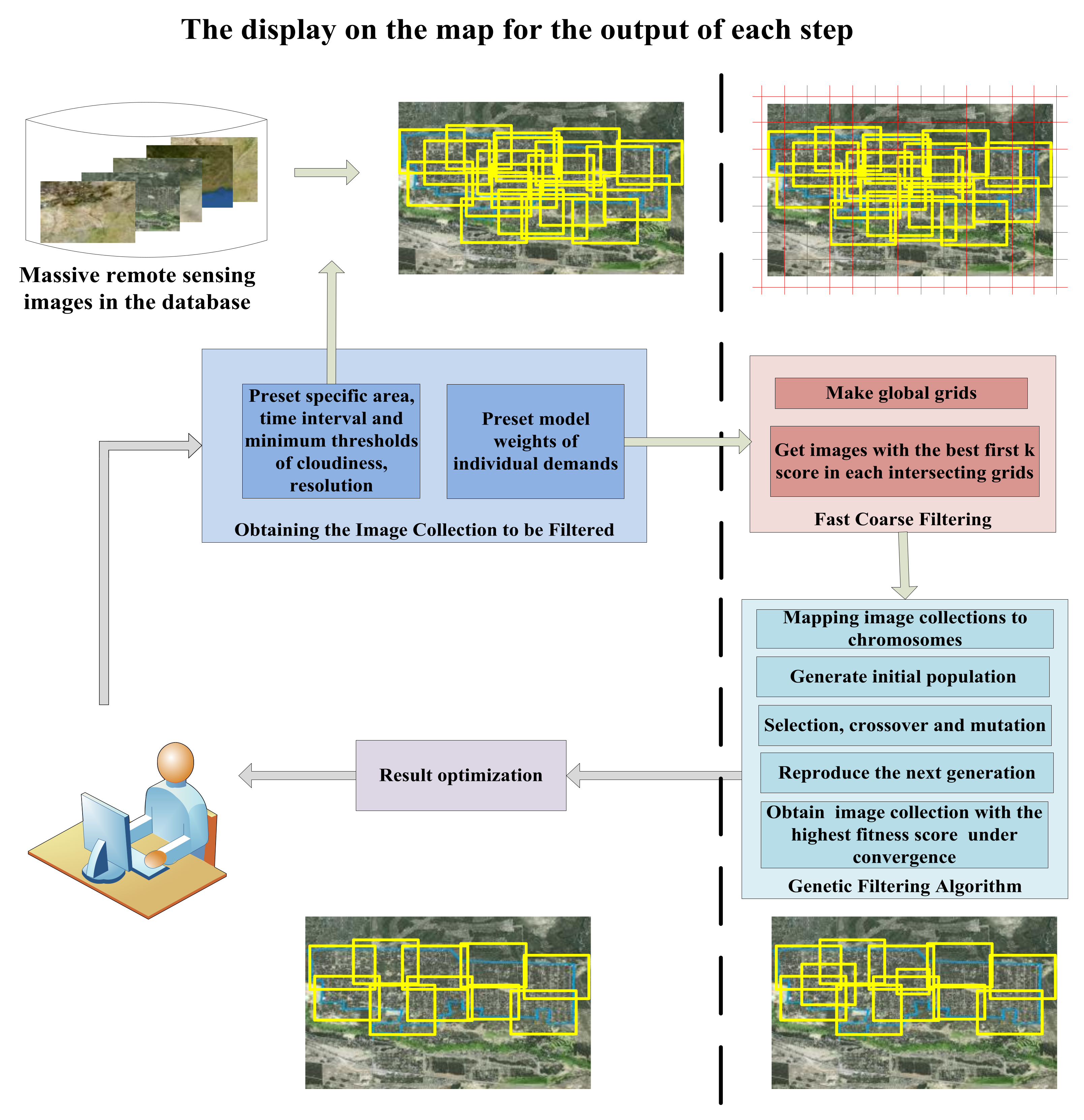
3. Proposed Method
3.1. Obtaining the Image Collection to Be Filtered
3.2. Fast, Coarse Filtering of the Image Collection
3.2.1. Creation of Global Grids
3.2.2. Coarse Filtering Based on Grids
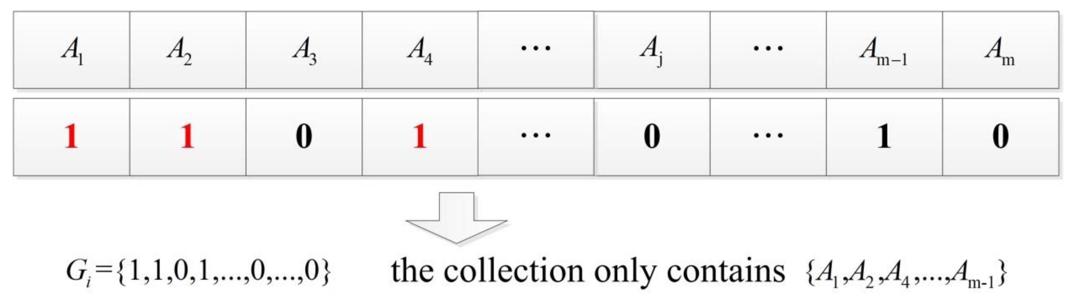
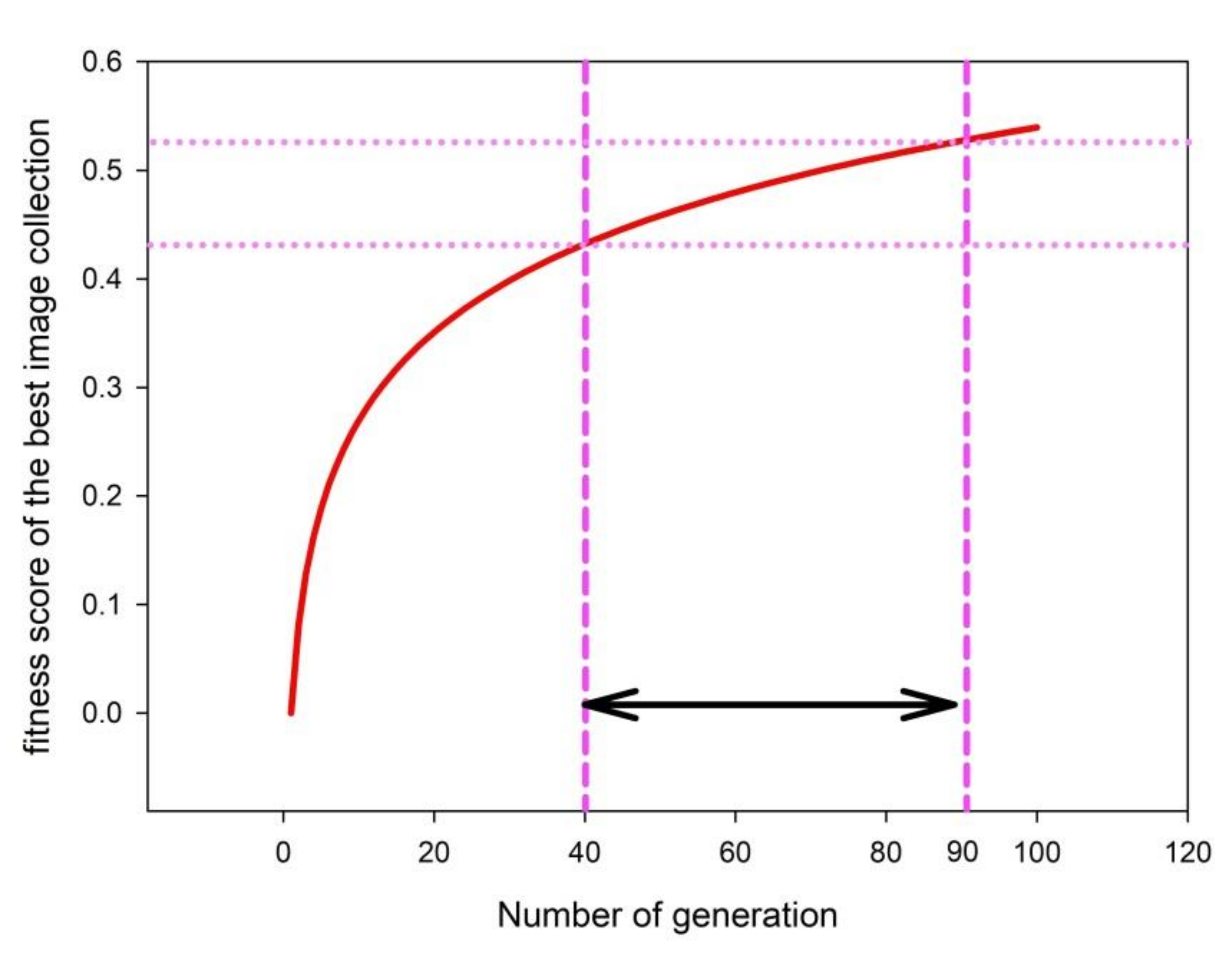
3.3. Further Filtering by the Genetic Algorithm
| Algorithm 1 Genetic Algorithm. |
| Input: Pc: possibility of cross Pm: possibility of mutation m: the number of genes in a population Output: optimal population 1: initialize population including m genes 2: calculate the fitness score for each gene 3: repeat 4: select m genes from population by using the roulette method 5: if(random(0,1) < Pc) { select two genes randomly cross between the two selected genes } 6: if(random(0,1) < Pm) { select one gene randomly mutation for this selected gene } 7: calculate fitness score for each gene 8: until(reaches stop condition) |
3.3.1. Population Initialization
3.3.2. Fitness Score Function
3.4. Filtering Result Optimization
4. Implementation and Performance Analysis
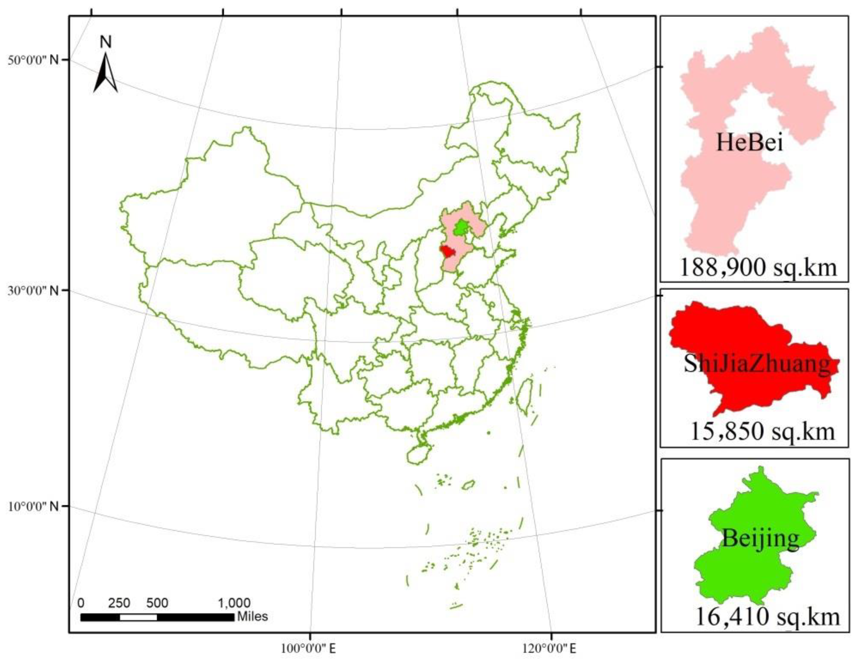
4.1. Experimental Region
4.2. Data
4.2.1. Data Source
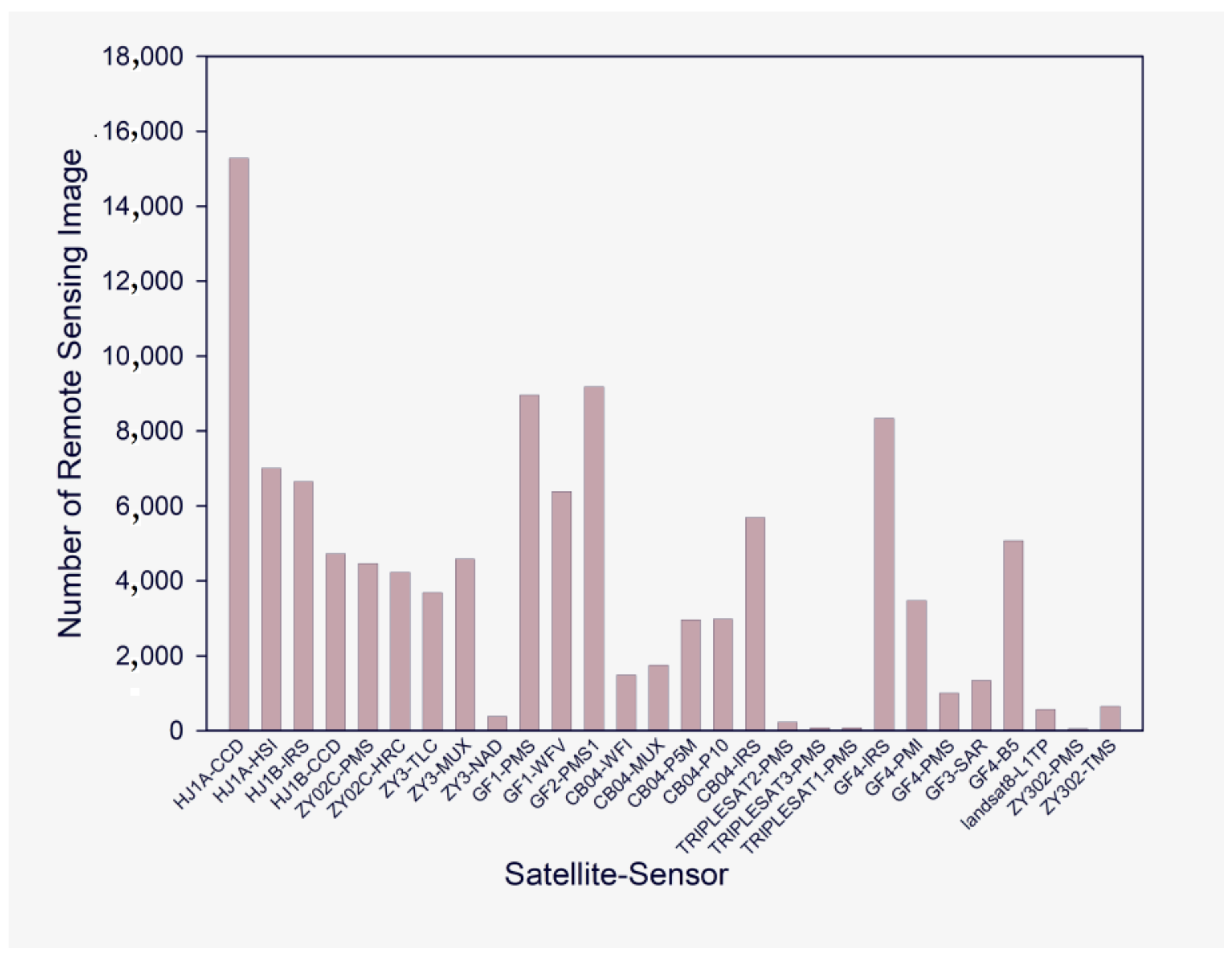
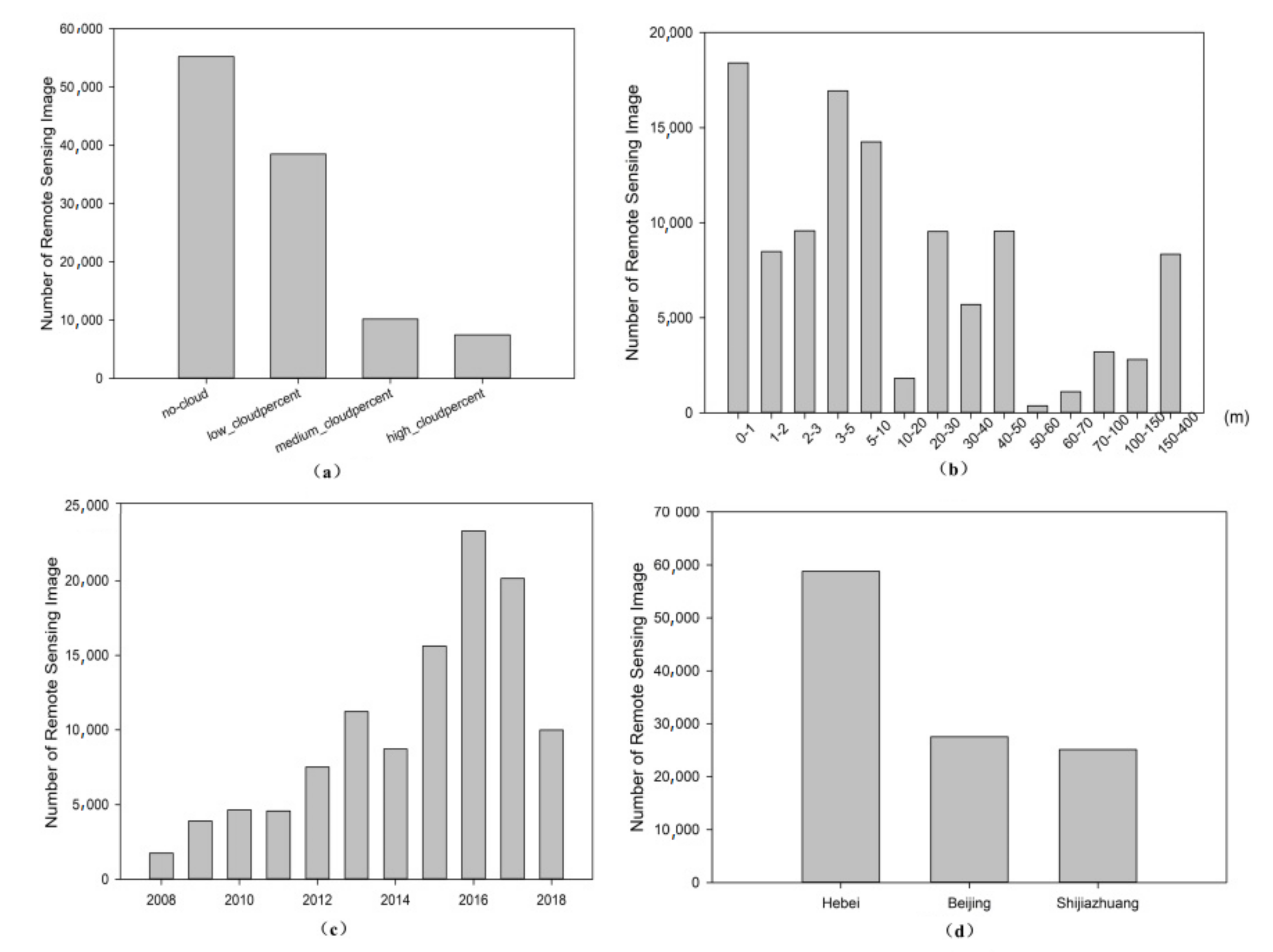
4.2.2. Image Data Distribution of Different Types and Regions
4.3. Experiment and Analysis
4.3.1. Experiments in Various Situations
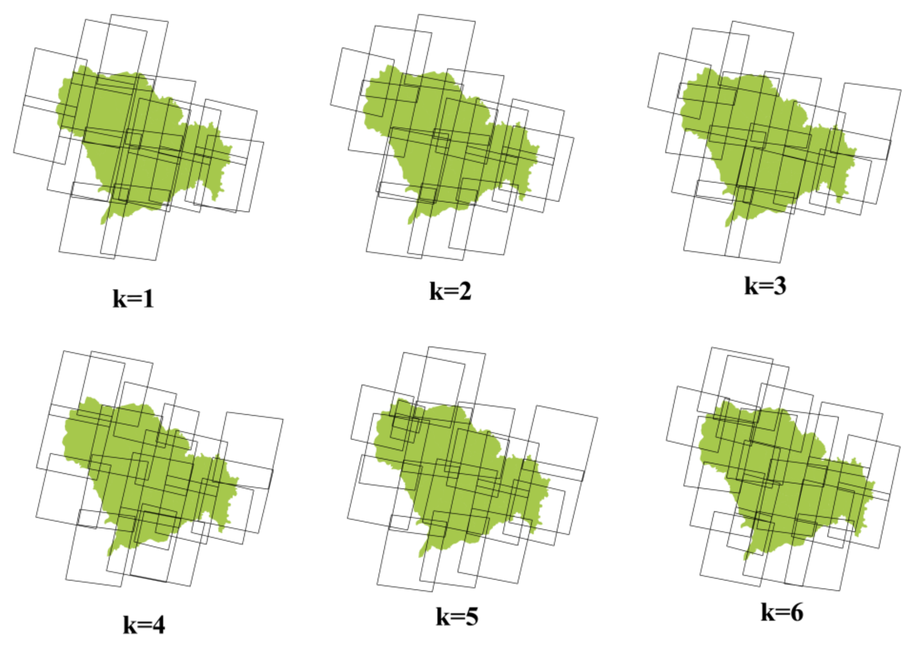
- a.
- Experimental results for different k values
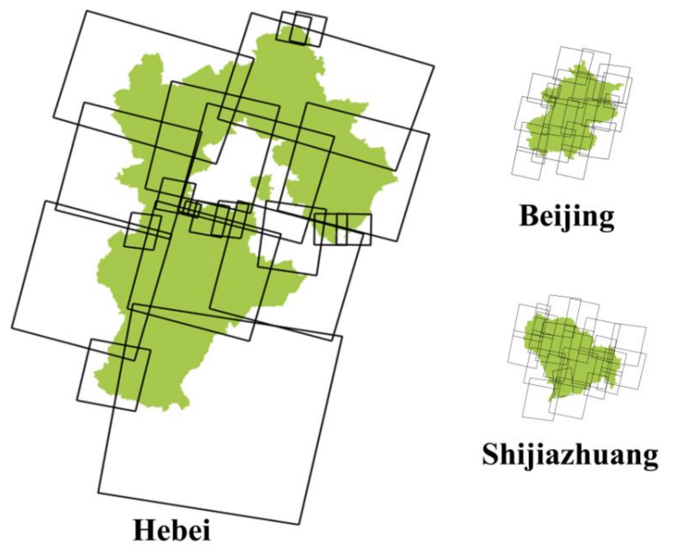
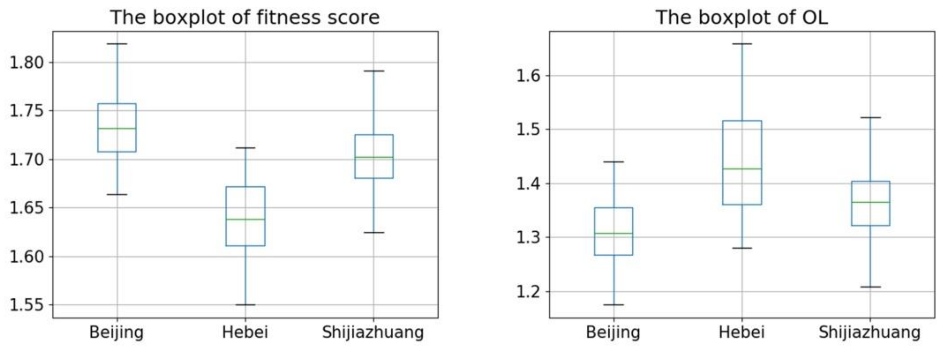
- b.
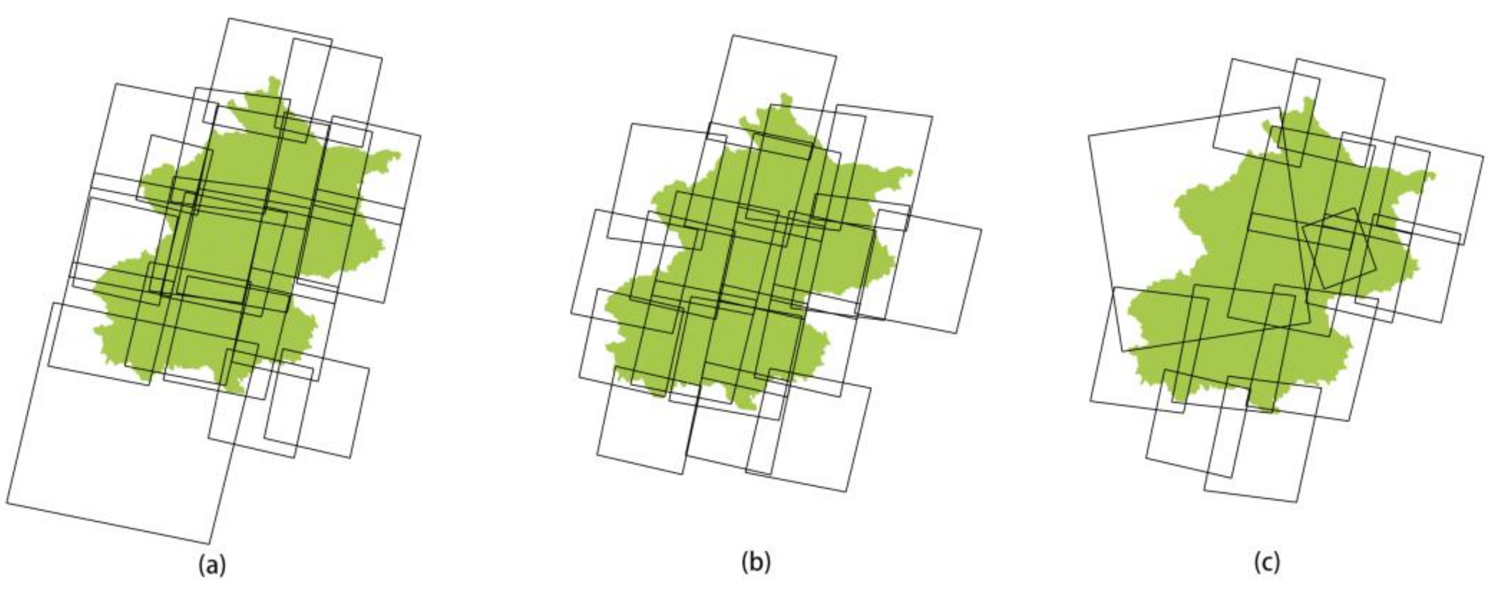
- Experimental results for different regions
- c.
- Experimental results for algorithm robustness verification
- d.
- Experimental results for different image numbers of
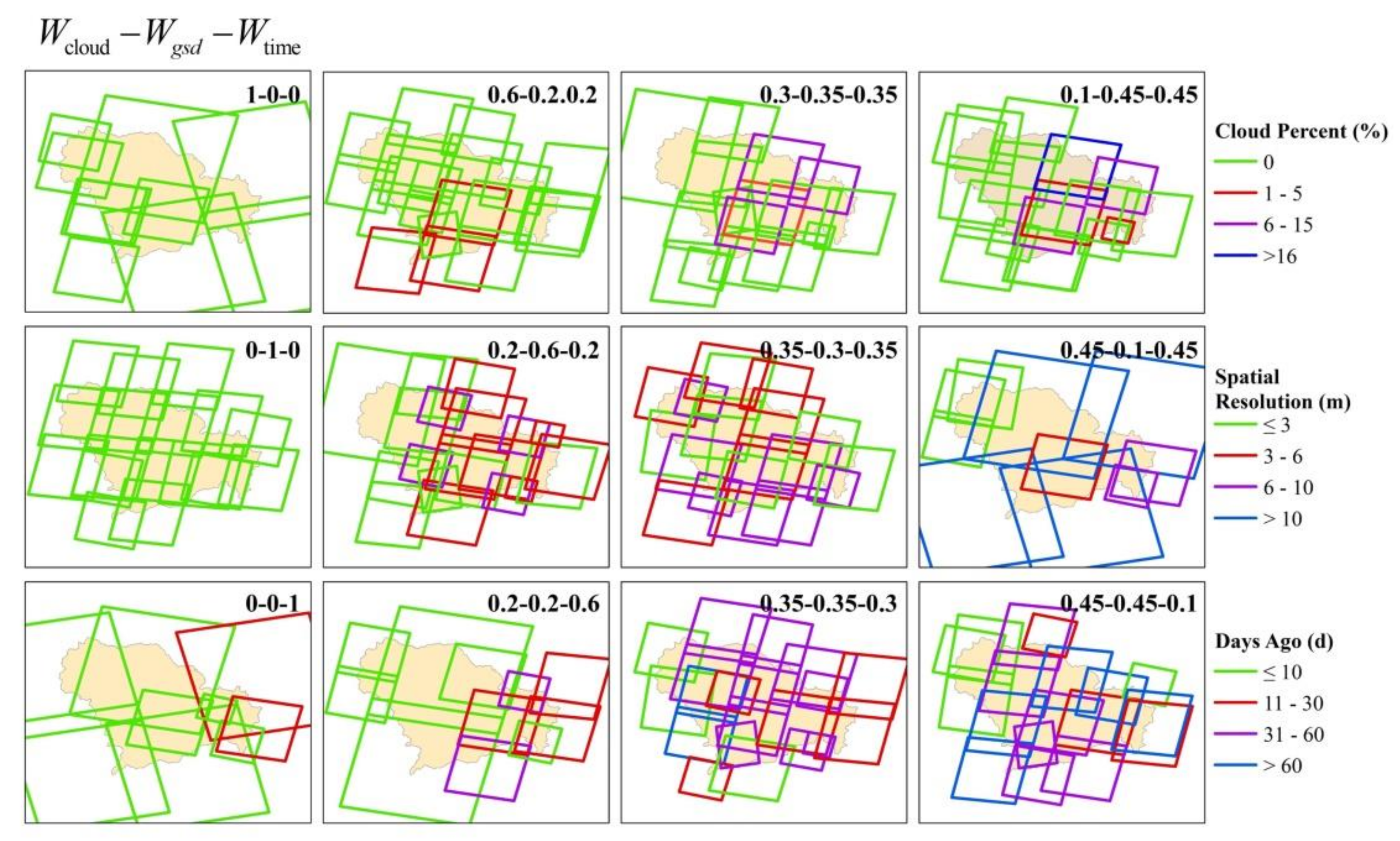
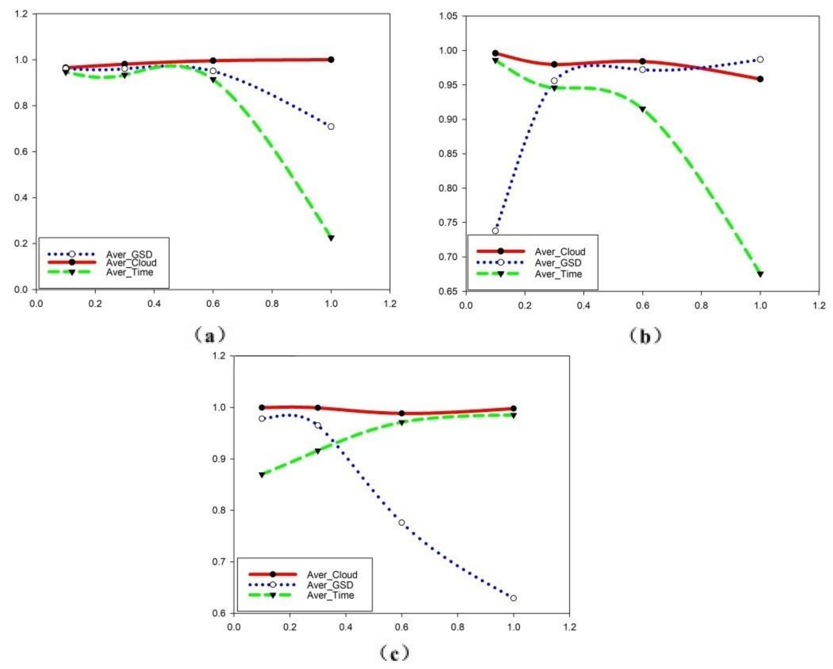
- e.
- Experimental results for individual demands
4.3.2. Comparison with Other Methods
5. Conclusions
Author Contributions
Funding
Institutional Review Board Statement
Informed Consent Statement
Acknowledgments
Conflicts of Interest
References
- Li, D.; Tong, Q.; Li, R.; Gong, J.; Zhang, L. Some frontier scientific issues of high-resolution earth observation. Sci. China Earth Sci. 2012, 42, 805–813. [Google Scholar] [CrossRef] [Green Version]
- Zhang, B. Current Status and Future Prospects of Remote Sensing. Bull. Chin. Acad. Sci. 2017, 32, 774–784. [Google Scholar]
- Li, J.; Hu, Q.; Ai, M. Optimal Illumination and Color Consistency for Optical RemoteSensing Image Mosaicking. IEEE Geosci. Remote Sens. Lett. 2017, 14, 1943–1947. [Google Scholar] [CrossRef]
- Sedaghat, A.; Ebadi, H. Remote Sensing Image Matching Based on Adaptive Binning SIFT Descriptor. IEEE Trans. Geosci. Remote Sens. 2015, 53, 5283–5293. [Google Scholar] [CrossRef]
- Xianyu, Z.; Minghao, X.; Xiangzhi, H.; Wenqian, Z.; Dongdong, S. A Full Coverage Retrieval Mode and Method for Remote Sensing Tile Data. J. Henan Univ. (Nat. Sci.) 2018, 48, 299–308. [Google Scholar]
- Han, L.; Pong, G.; Jie, W.; Nicholas, C.; Yuqi, B.; Shunlin, L. Annual dynamics of global land cover and its long-term changes from 1982 to 2015. Earth Syst. Sci. Data 2020, 2, 1217–1243. [Google Scholar] [CrossRef]
- Zhang, X.; Liu, L.; Chen, X.; Gao, Y.; Xie, S.; Mi, J. GLC_FCS30: Global land-cover product with fine classification system at 30 m using time-series Landsat imagery. Earth Syst. Sci. Data 2021, 13, 2753–2776. [Google Scholar] [CrossRef]
- Zhang, X.; Liu, L.; Chen, X.; Gao, Y.; Jiang, M. Automatically Monitoring Impervious Surfaces Using Spectral Generalization and Time Series Landsat Imagery from 1985 to 2020 in the Yangtze River Delta. J. Remote Sens. 2021, 2021, 873816. [Google Scholar] [CrossRef]
- Wang, D.L.; Hu, F. Monitoring of illegal buildings in Beijing using high-resolution satellite imagery from China. Chin. Sci. Bull. 2009, 54, 305–311. [Google Scholar] [CrossRef]
- Moghadam, N.K.; Delavar, M.R.; Hanachee, P. Automatic urban illegal building detection using multi-temporal satellite images and geospatial information systems. ISPRS—Int. Arch. Photogramm. Remote Sens. Spat. Inf. Sci. 2015, XL-1-W5, 387–393. [Google Scholar] [CrossRef] [Green Version]
- Hu, F.; Xia, G.S.; Zhang, L. Deep sparse representations for land-use scene classification in remote sensing images. In Proceedings of the 2016 IEEE 13th International Conference on Signal Processing (ICSP), Chengdu, China, 6–10 November 2016. [Google Scholar]
- Li, Y.; Zhang, Y.; Huang, X.; Zhu, H.; Ma, J. Large-Scale Remote Sensing Image Retrieval by Deep Hashing Neural Networks. IEEE Trans. Geosci. Remote Sens. 2018, 56, 950–965. [Google Scholar] [CrossRef]
- Li, J.; Shen, B.; Jiang, R.; Chen, T. Quadtree Spatial Index Algorithm for Image Pyramid. Comput. Eng. 2011, 37, 11–13. [Google Scholar]
- Cheng, G.; Han, J.W.; Lu, X.Q. Remote Sensing Image Scene Classification: Benchmark and State of the Art. Proc. IEEE 2017, 105, 1865–1883. [Google Scholar] [CrossRef] [Green Version]
- Egenhofer, M.J. Spatial-Query-by-Sketch. In Proceedings of the IEEE Symposium on Visual Languages, Washington, DC, USA, 3 October 1996. [Google Scholar]
- Lee, Y.C.; Chin, F.L. An iconic query language for topological relationships in GIS. Int. J. Geogr. Inf. Syst. 1995, 9, 25–46. [Google Scholar] [CrossRef]
- Shekhar, S.; Chawla, S.; Ravada, S.; Fetterer, A.; Liu, X.; Lu, C. Spatial databases-accomplishments and research needs. Knowledge and Data Engineering. IEEE Trans. 1999, 11, 45–55. [Google Scholar]
- Gaede, V.; Günther, O. Multidimensional access methods. ACM Comput. Surv. 1998, 30, 170–231. [Google Scholar] [CrossRef]
- Aptoula, E. Remote Sensing Image Retrieval with Global Morphological Texture Descriptors. IEEE Trans. Geosci. Remote Sens. 2014, 52, 3023–3034. [Google Scholar] [CrossRef]
- Li, F.; You, S.; Wei, H.; Wei, E.; Chen, L. Filtering model of optimal dataset for remote sensing image area coverage. Radio Eng. 2017, 47, 45–48. [Google Scholar]
- Maulik, U.; Bandyopadhyay, S. Fuzzy partitioning using a real-coded variable-length genetic algorithm for pixel classification. IEEE Trans. Geosci. Remote Sens. 2003, 41, 1075–1081. [Google Scholar] [CrossRef]
- Stavrakoudis, D.; Theocharis, J.; Zalidis, G. A Boosted Genetic Fuzzy Classifier for land cover classification of remote sensing imagery. ISPRS J. Photogramm. Remote Sens. 2011, 66, 529–544. [Google Scholar] [CrossRef]
- Tseng, M.-H.; Chen, S.-J.; Hwang, G.-H.; Shen, M.-Y. A genetic algorithm rule-based approach for land-cover classification. ISPRS J. Photogramm. Remote Sens. 2008, 63, 202–212. [Google Scholar] [CrossRef]
- Nikfar, M.; Zoej, M.J.V.; Mohammadzadeh, J.; Mokhtarzade, M.; Navabi, A. Optimization of multiresolution segmentation by using a genetic algorithm. J. Appl. Remote Sens. 2012, 6, 063592. [Google Scholar] [CrossRef]
- Krawiec, K.; Bhanu, B. Visual learning by coevolutionary feature synthesis. IEEE Trans. Syst. Man Cybern. Part B (Cybernetics) 2005, 35, 409–425. [Google Scholar] [CrossRef]
- Pedergnana, M.; Marpu, P.R.; Mura, M.D.; Benediktsson, J.A.; Bruzzone, L. A Novel Technique for Optimal Feature Selection in Attribute Profiles Based on Genetic Algorithms. IEEE Trans. Geosci. Remote Sens. 2013, 51, 3514–3528. [Google Scholar] [CrossRef]
- Puig, D.; Garcia, M.A. Automatic texture feature selection for image pixel classification. Pattern Recognit. 2006, 39, 1996–2009. [Google Scholar] [CrossRef]
- Ines, A.V.; Honda, K. On quantifying agricultural and water management practices from low spatial resolution RS data using genetic algorithms: A numerical study for mixed-pixel environment. Adv. Water Resour. 2005, 28, 856–870. [Google Scholar] [CrossRef] [Green Version]
- Zhan, H.; Lee, Z.; Shi, P.; Chen, C.; Carder, K. Retrieval of water optical properties for optically deep waters using genetic algorithms. IEEE Trans. Geosci. Remote Sens. 2003, 41, 1123–1128. [Google Scholar] [CrossRef]


| Parameter | Definition |
|---|---|
| Target_Area | Specific area preset by users. The goal of the LFCF-ID is to filter and obtain the full-coverage image collection of this area |
| , | The time interval is preset by users to obtain the images to be filtered |
| The lowest image resolution that the user can accept in the filter result | |
| The highest image cloudiness that the user can accept in the filtered result | |
| The lowest coverage that the user can accept | |
| The user’s demand weight for the spatial resolution of the image | |
| The user’s demand weight for the image cloudiness | |
| The user’s demand weight for the timeliness of the image |
| Name of Satellite | Sensor Type | Resolution | Width |
|---|---|---|---|
| GaoFen1 | Multispectral | 2/8 m | 60 km |
| GaoFen2 | Multispectral | 1/4 m | 45 km |
| GaoFen3 | SAR | 1–500 m | 5–650 km |
| GaoFen4 | Multispectral/infrared | 50/400 m | 400 km |
| ZiYuan3-02C | Multispectral | 5/10 m | 51 km |
| ZiYuan3 | Multispectral | 2.1 m | 51 km |
| ZiYuan-CB04 | Multispectral | 2.36 m | 113 km |
| Huanjing-1A | Multispectral/hyperspectral | 30/100 m | 360/50 km |
| Huanjing-1B | Multispectral/infrared | 30/300 m | 360/720 km |
| TRIPLESAT1 | Multispectral | 0.8/3.2 m | 51 km |
| TRIPLESAT2 | Multispectral | 0.8 m/3.2 m | 51 km |
| TRIPLESAT3 | Multispectral | 0.8 m/3.2 m | 51 km |
| LANDSAT8-L1TP | Multispectral/infrared | 15/30/100 m | 185 km |
| k | |||
|---|---|---|---|
| 1 | 29 | 1.661959 | 19 |
| 2 | 56 | 1.687312 | 18 |
| 3 | 75 | 1.732062 | 17 |
| 4 | 101 | 1.728173 | 19 |
| 5 | 133 | 1.716126 | 20 |
| 6 | 163 | 1.691373 | 21 |
| Study Area | Area (km2) | Time Consumption (s) | |||
|---|---|---|---|---|---|
| Shijiazhuang | 15,850 | 100% | 23 | 1.320225 | 3.1044 |
| Beijing | 16,410 | 100% | 22 | 1.243119 | 3.8220 |
| Hebei | 188,900 | 100% | 21 | 1.432177 | 68.6900 |
| Image Number of | Time Consumption (s) | |||
|---|---|---|---|---|
| 243 | 14.93578 | 1.557944 | 1.633028 | 2.886000156402588 |
| 486 | 20 | 1.566519 | 1.394495 | 7.019999980926514 |
| 626 | 35.78899 | 1.584082 | 1.426606 | 3.6347999572753906 |
| 710 | 39.62844 | 1.705311 | 1.353211 | 3.5411999225616455 |
| 867 | 45.72477 | 1.600818 | 1.490826 | 4.648799896240234 |
| 1202 | 60.09174 | 1.60953 | 1.522936 | 2.683199882507324 |
| 1928 | 97.96789 | 1.682792 | 1.385321 | 2.8703999519348145 |
| 2982 | 146.2477 | 1.792568 | 1.224771 | 3.75959992408752 |
| 4094 | 198.2018 | 1.691633 | 1.408257 | 5.50679993629455 |
| 4955 | 240.4128 | 1.689813 | 1.40367 | 4.040399789810181 |
| 5975 | 289.156 | 1.735492 | 1.325688 | 5.756400108337402 |
| 6935 | 333.2982 | 1.753975 | 1.261468 | 5.30400013923645 |
| 7994 | 379.8945 | 1.762623 | 1.256881 | 4.055999994277954 |
| 9019 | 426.5505 | 1.715952 | 1.348624 | 6.910799980163574 |
| 10008 | 500.2661 | 1.750479 | 1.307339 | 8.252399921417236 |
| Fitness Score | Aver_Cloud | Aver_GSD | Aver_Time | |||
|---|---|---|---|---|---|---|
| 1 | 0 | 0 | 1.67424 | 1 | 0.708643 | 0.225515 |
| 0.6 | 0.2 | 0.2 | 1.70223 | 0.995618 | 0.95063 | 0.915011 |
| 0.3 | 0.35 | 0.35 | 1.7221 | 0.980618 | 0.960834 | 0.934039 |
| 0.1 | 0.45 | 0.45 | 1.67466 | 0.965056 | 0.961545 | 0.946545 |
| 0 | 1 | 0 | 1.73802 | 0.958371 | 0.986794 | 0.675474 |
| 0.2 | 0.6 | 0.2 | 1.69685 | 0.983989 | 0.97199 | 0.915378 |
| 0.35 | 0.3 | 0.35 | 1.68953 | 0.979607 | 0.95591 | 0.945887 |
| 0.45 | 0.1 | 0.45 | 1.66885 | 0.995955 | 0.737714 | 0.986116 |
| 0 | 0 | 1 | 1.67702 | 0.99764 | 0.629191 | 0.985105 |
| 0.2 | 0.2 | 0.6 | 1.74005 | 0.988258 | 0.775825 | 0.971083 |
| 0.35 | 0.35 | 0.3 | 1.76462 | 0.999101 | 0.964984 | 0.915991 |
| 0.45 | 0.45 | 0.1 | 1.70676 | 0.999494 | 0.977812 | 0.869792 |
| Manual Filtering Method | Greedy Method | LFCF-ID (k = 1) | LFCF-ID (k = 3) | |||||
|---|---|---|---|---|---|---|---|---|
| Study Area | Time Consumption (s) | Fitness Score | Time Consumption (s) | Fitness Score | Time Consumption (s) | Fitness Score | Time Consumption (s) | Fitness Score |
| Shijiazhuang | 48.986 | 1.7021 | 0.3432 | 1.4726 | 1.9032 | 1.6988 | 3.1044 | 1.7218 |
| Beijing | 100.738 | 1.6818 | 0.5460 | 1.4611 | 2.4336 | 1.7093 | 3.8220 | 1.7315 |
| Hebei | 652.584 | 1.6492 | 8.0340 | 1.3015 | 30.1704 | 1.6176 | 68.6900 | 1.6708 |
Publisher’s Note: MDPI stays neutral with regard to jurisdictional claims in published maps and institutional affiliations. |
© 2021 by the authors. Licensee MDPI, Basel, Switzerland. This article is an open access article distributed under the terms and conditions of the Creative Commons Attribution (CC BY) license (https://creativecommons.org/licenses/by/4.0/).
Share and Cite
Chu, B.; Gao, F.; Chai, Y.; Liu, Y.; Yao, C.; Chen, J.; Wang, S.; Li, F.; Zhang, C. Large-Area Full-Coverage Remote Sensing Image Collection Filtering Algorithm for Individual Demands. Sustainability 2021, 13, 13475. https://0-doi-org.brum.beds.ac.uk/10.3390/su132313475
Chu B, Gao F, Chai Y, Liu Y, Yao C, Chen J, Wang S, Li F, Zhang C. Large-Area Full-Coverage Remote Sensing Image Collection Filtering Algorithm for Individual Demands. Sustainability. 2021; 13(23):13475. https://0-doi-org.brum.beds.ac.uk/10.3390/su132313475
Chicago/Turabian StyleChu, Boce, Feng Gao, Yingte Chai, Yu Liu, Chen Yao, Jinyong Chen, Shicheng Wang, Feng Li, and Chao Zhang. 2021. "Large-Area Full-Coverage Remote Sensing Image Collection Filtering Algorithm for Individual Demands" Sustainability 13, no. 23: 13475. https://0-doi-org.brum.beds.ac.uk/10.3390/su132313475