Article

Simulation-Optimization for the Planning of Off-Site Construction Projects: A Comparative Study of Recent Swarm Intelligence Metaheuristics

1
Department of Building and Real Estate, The Hong Kong Polytechnic University, Hong Kong 999077, China
2
Civil Engineering Department, Faculty of Engineering, Assiut University, Assiut 71511, Egypt
3
Department of Industrial and Systems Engineering, The Hong Kong Polytechnic University, Hong Kong 999077, China
4
Department of Industrial and Manufacturing Engineering, Egypt-Japan University of Science and Technology (E-JUST), New Borg El Arab 21934, Egypt
*
Author to whom correspondence should be addressed.
Sustainability 2021, 13(24), 13551; https://0-doi-org.brum.beds.ac.uk/10.3390/su132413551
Submission received: 11 September 2021 / Revised: 25 November 2021 / Accepted: 2 December 2021 / Published: 7 December 2021

Abstract

:
Off-site construction is a modern construction method that brings many sustainability merits to the built environment. However, the sub-optimal planning decisions (e.g., resource allocation, logistics and overtime planning decisions) of off-site construction projects can easily wipe away their sustainability merits. Therefore, simulation modelling—an efficient tool to consider the complexity and uncertainty of these projects—is integrated with metaheuristics, developing a simulation-optimization model to find the best possible planning decisions. Recent swarm intelligence metaheuristics have been used to solve various complex optimization problems. However, their potential for solving the simulation-optimization problems of construction projects has not been investigated. This research contributes by investigating the status-quo of simulation-optimization models in the construction field and comparing the performance of five recent swarm intelligence metaheuristics to solve the stochastic time–cost trade-off problem with the aid of parallel computing and a variance reduction technique to reduce the computation time. These five metaheuristics include the firefly algorithm, grey wolf optimization, the whale optimization algorithm, the salp swarm algorithm, and one improved version of the well-known bat algorithm. The literature analysis of the simulation-optimization models in the construction field shows that: (1) discrete-event simulation is the most-used simulation method in these models, (2) most studies applied genetic algorithms, and (3) very few studies used computation time reduction techniques, although the simulation-optimization models are computationally expensive. The five selected swarm intelligence metaheuristics were applied to a case study of a bridge deck construction project using the off-site construction method. The results further show that grey wolf optimization and the improved bat algorithm are superior to the firefly, whale optimization, and salp swarm algorithms in terms of the obtained solutions’ quality and convergence behaviour. Finally, the use of parallel computing and a variance reduction technique reduces the average computation time of the simulation-optimization models by about 87.0%. This study is a step towards the optimum planning of off-site construction projects in order to maintain their sustainability advantages.

1. Introduction

Off-site construction (OSC) is a sustainable construction method in which parts of the structure are produced off-site and then transported to the construction site for erection [1,2]. OSC has many advantages for the improvement of productivity [3], quality [4], and safety [5] of the built environment. Besides this, OSC brings environmental improvements to the construction industry [6]. OSC could reduce greenhouse gas (GHG) emissions by 48% and 43% during the operation and construction phases, respectively [7]. Furthermore, OSC could reduce construction waste compared with traditional construction [8]. Consequently, OSC is adopted in both building and infrastructure projects. For instance, OSC is an efficient way to narrow the gap between the supply and demand of both public and private buildings [9]. In addition, many transportation agencies prefer OSC to deliver infrastructure projects to mitigate the traffic interruption resulting from the traditional cast-in-situ method [10].
Despite the benefits of OSC, its complexity and fragmentation require extensive planning from the project managers [1,11]. The need for extensive planning is one of the key barriers that hinder the wider adoption of OSC [12]. For successful project delivery, the project manager has to make critical decisions while considering the dynamics and uncertainty of OSC projects [13]. Some of these decisions are related to resource planning, such as the number of required crews and the on-site and off-site equipment [14]. The rest are related to logistics aspects, such as the location of the storage yards and their capacities. These decisions should be made to deliver the project on time and within the allowable budget. This problem is called the time–cost trade-off problem (TCTP), which has been extensively addressed in the literature considering its different variants and has been solved using both exact and approximate optimization methods. Approximate methods are preferable because they efficiently handle complex projects with large networks in a reasonable computation time [15]. Metaheuristics were widely used to solve single and multi-objective TCTP. The Genetic Algorithm (GA) [16], Ant Colony Optimization (ACO) [17], and Particle Swarm Optimization (PSO) [18] were applied to solve single-objective TCTP. For multi-objective TCTP, researchers used dynamic programming [19], multi-objective ACO [20], non-dominated sorting genetic algorithm II (NSGA-II), multi-objective simulated annealing, and multi-objective PSO [21]. Despite the contribution of these studies, their common limitations are: (1) The proposed models addressed the traditional cast-in-situ construction method. Hence, they do not fit with OSC projects characterized by a three-stage supply chain (i.e., production, logistics, and installation stages) [22]. (2) The previous models failed to capture the complex interactions between the resources and activities of OSC projects. These complex interactions form queues inside the system, making the analytical methods impractical for the modelling of such queuing systems [23]. (3) the previous models assumed that the activities’ durations and costs are deterministic without considering the uncertainty associated with these types of projects [24].
In order to address these gaps, researchers resorted to Discrete-Event Simulation (DES) to capture the complexity and uncertainty of OSC projects without the need to develop sophisticated mathematical models. However, DES is not an optimization tool on its own; it can solely enable project planners to study the effect of the proposed resource planning and logistics decisions on the project duration, cost and productivity [10]. In order to tackle this limitation, researchers tend to combine simulation and metaheuristics into one approach called “simulation-optimization (SO)”. Swisher et al. [25] defined SO as a ‘‘structured approach to determine optimal input parameter values, where optimal is measured by a function of output variables—steady-state or transient—associated with a simulation model’’. Given this definition, the solution obtained from the SO approach is the values of the input parameters associated with the DES model. This solution’s performance is evaluated by the DES model. The metaheuristic algorithm uses the current solution and its evaluation to find a new set of input values [26]. Therefore, different types of metaheuristics have been integrated with DES in the SO approach to solve multiple construction problems characterized by complexity and uncertainty.
Evolution-based metaheuristics are a subcategory of metaheuristics inspired by the laws of natural evolution. The advantage of these metaheuristics is that the new generation of solutions is created using the fittest solutions in the current generation, hence improving the solutions over the generations [27]. Genetic Algorithms (GAs), which are the most popular evolution-based metaheuristics, have frequently been used in SO for different construction applications such as sewer pipeline installation [28], earthmoving operations [29], the production planning of precast components [30], the planning of prefabricated building construction [31], and bridge construction planning [32].
Swarm Intelligence (SI) metaheuristics are another subcategory of metaheuristics. These metaheuristics are usually inspired by the social and hunting behaviours of colonies and swarms of animals in nature. According to Mirjalili et al. [33], SI metaheuristics offer multiple advantages over evolution-based metaheuristics. Firstly, they retain the information associated with the search space over iterations, while evolution-based metaheuristics dispose the information of previous generations once a new generation is created. Secondly, they are generally easier to implement because they have fewer operators than the evolution-based metaheuristics (i.e., operators for crossover, mutation, elitism, etc.). Despite these advantages, SI metaheuristics have rarely been used in SO for construction applications. Examples of these applications are a concrete placement operation using PSO [34], and the construction planning of bridge deck construction using ACO [35] and PSO [36]. Because of the introduction of PSO and ACO, SI metaheuristics have witnessed a dramatic development, leading to tens of metaheuristics that have potential over PSO and ACO, while most of them use a lower number of tuning parameters. Examples of such recent SI metaheuristics are the firefly algorithm (FA) [37], grey wolf optimization (GWO) [38], the whale optimization algorithm (WOA) [39] and the salp swarm algorithm (SSA) [40].
Given the above-mentioned preliminary review of the use of metaheuristics in SO in the construction domain, this study contributes to the literature by addressing three research questions that have not yet been addressed: (1) What is the status quo of the use of metaheuristics for SO in the construction research field? (2) What is the potential of the use of recent SI metaheuristics in SO to optimize the planning of OSC projects? (3) Which one among the selected SI metaheuristics has better performance in obtaining more optimal planning decisions for OSC? In order to address these questions, the metaheuristics used in the SO of construction applications are first reviewed using a systematic review. Secondly, a DES model of a bridge construction project using the OSC method is developed. Then, its optimization model is formulated by defining the decision variables, objective functions and constraints. Next, the developed model is integrated with the SI metaheuristics under study. In order to reduce the computation time of the SO runs, parallel computing and a variance reduction technique called common rand numbers (CRN) are used. After that, the developed models are applied to a case study. Finally, a comparative analysis between the SI metaheuristics under study is conducted using qualitative and quantitative measures. Following the recommendations of Sörensen [41] and Juan et al. [26] regarding the need to conduct comparative studies for SO, this study contributes by comparing the performance of recent SI metaheuristics in SO of OSC projects.
The rest of this study is organized as follows: SO applications in the construction field are reviewed in Section 2. Secondly, the problem description and the formulation of the optimization model are discussed in Section 3. Thirdly, the adopted SO approach, the DES modelling of an OSC project, and the five SI metaheuristics under study are illustrated and coded in Section 4, including their parameter tuning. In addition, Section 4 elaborates on the methods used to reduce the computation time, namely, the CRN method and parallel computing. After that, the developed simulation and optimization models are applied to a case study discussed in Section 5. Finally, the analysis and discussion of the performance of the SI metaheuristics are provided in Section 6 in terms of their convergence behaviour and statistical results, followed by conclusions in Section 7.

2. Literature Review of Simulation-Optimization (SO) in the Construction Research Field

This section answers the first research question mentioned in the previous section by reviewing the SO applications in the construction research field. The specific aims are the identification of: (1) studies that adopted SO in the construction domain, (2) which simulation methods (e.g., DES, agent-based simulation (ABS), system dynamics (SD)) have been used in these studies, (3) which metaheuristics have been applied in these studies, (4) the construction applications addressed, and (5) whether these studies applied parallel computing or VRTs. These objectives can be applied using a systematic review method [42,43]. This method consists of two main steps: the extraction of related studies and their analysis [44]. The first step starts by selecting a number of relevant keywords for the database search. The following search code was used in the Scopus database: (TITLE-ABS-KEY (“optimization”) AND TITLE-ABS-KEY (“construction”) OR TITLE-ABS-KEY (“infrastructure”) OR TITLE-ABS-KEY (“building”) AND TITLE-ABS-KEY (“simulation”) AND TITLE-ABS-KEY (“DES”) OR TITLE-ABS-KEY (“discrete”) OR TITLE-ABS-KEY (“continuous”) OR TITLE-ABS-KEY (“discrete-event”) OR TITLE-ABS-KEY (“system dynamic”) OR TITLE-ABS-KEY (“system dynamics”) OR TITLE-ABS-KEY (“SD”) OR TITLE-ABS-KEY (“agent”) OR TITLE-ABS-KEY (“multi-agent”) OR TITLE-ABS-KEY (“agent-based”) OR TITLE-ABS-KEY (“ABS”) OR TITLE-ABS-KEY (“ABM”)) AND (LIMIT-TO (DOCTYPE, “ar”)) AND (LIMIT-TO (LANGUAGE, “English”)) AND (EXCLUDE (SUBJAREA, “MATE”) OR EXCLUDE (SUBJAREA, “PHYS”) OR EXCLUDE (SUBJAREA, “EART”) OR EXCLUDE (SUBJAREA, “CHEM”) OR EXCLUDE (SUBJAREA, “CENG”) OR EXCLUDE (SUBJAREA, “BIOC”) OR EXCLUDE (SUBJAREA, “MEDI”) OR EXCLUDE (SUBJAREA, “PHAR”) OR EXCLUDE (SUBJAREA, “AGRI”) OR EXCLUDE (SUBJAREA, “NEUR”) OR EXCLUDE (SUBJAREA, “IMMU”) OR EXCLUDE (SUBJAREA, “HEAL”) OR EXCLUDE (SUBJAREA, “ARTS”) OR EXCLUDE (SUBJAREA, “NURS”) OR EXCLUDE (SUBJAREA, “PSYC”)). As of November 2021, using this code results in the identification of 745 studies, as shown in Figure 1. Figure 1 shows a common protocol used in the systematic review, called the Preferred Reporting Items for Systematic Reviews and Meta-Analyses (PRISMA), to screen the relevant studies [45]. After checking the title and abstract of the retrieved studies, 637 studies were found to be irrelevant to the construction research field, namely the implementation stage of construction projects. Then, the full texts of the remaining studies (i.e., 745 – 637 = 108 studies) were evaluated, and 38 of them were found to be relevant. By checking the reference list and studies that cited each of the 38 studies, eight more relevant studies were detected, raising the number of related studies to 46, as shown in Figure 1.
The second step of the adopted systematic review method is to evaluate the 46 relevant studies to identify the simulation methods and metaheuristics used, their applications, and the use of parallel computing and VRTs. 
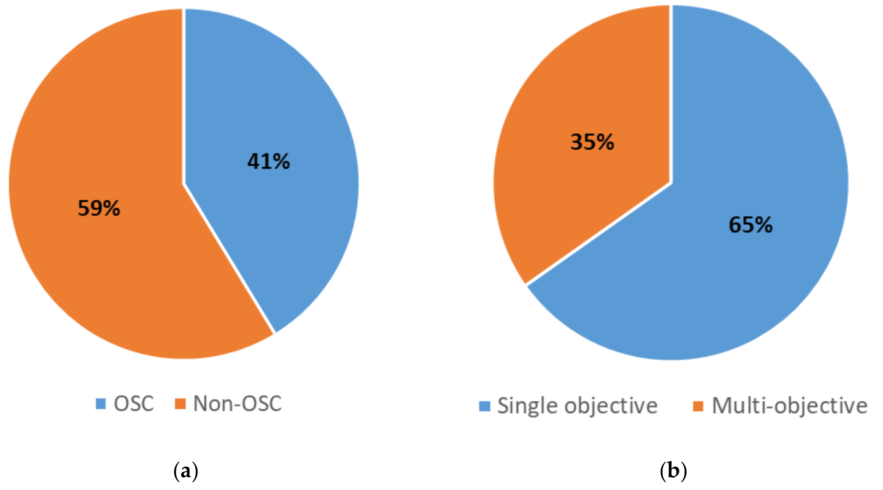
Figure 2 provides an overview of the classification of the 46 studies based on multiple criteria. Figure 2a shows that most of these studies (59%) are related to the traditional construction method, while Figure 2b shows that 65% of these studies addressed single optimization problems. Regarding the metaheuristics used in these studies, Figure 2c shows that the majority of these studies used evolutionary-based metaheuristics (i.e., GA and evolutionary algorithms (EA)), while one-fifth of these studies adopted SI metaheuristics (i.e., PSO and ACO). Table 1 provides details of this information, including the adoption of parallel computing and VRTs to reduce the computation time, as well as the type of simulation methods used in these studies. Most of these studies integrated DES with optimization, while very few studies conducted SO using ABS and SD, as shown in Table 1. Furthermore, Table 1 shows that three studies used parallel computing, while only one study adopted VRTs. Despite the vast improvements in computing power, computation time reduction is inevitable for five reasons: (1) Construction projects are usually characterized by uncertainty. For example, their activities’ durations are best represented by probabilistic distributions; hence, multiple simulation replications are required to obtain reliable results, which in turn prolong the computation time. (2) SO with metaheuristics requires the call of the simulation model frequently to evaluate the fitness of each individual solution of the population in each iteration. (3) Finding the optimum values of the controllable parameters for each metaheuristic requires extensive numerical experiments. (4) Construction researchers tend to hybridize DES with other simulation approaches such as system dynamics [46] or integrate it with neural networks [47]. Such research developments would increase the capabilities of DES but at the expense of the computation time. (5) OSC projects are dynamic in nature, meaning that optimized decisions made in the early planning stage might be infeasible in later construction stages due to inevitable uncertainties [32]. Therefore, there is a need to make near-optimum planning decisions in a reasonable computation time.
Given the above analysis of the literature of SO in the construction domain, a number of research gaps were identified. Firstly, most of the studies used traditional SO methods by solely integrating DES and metaheuristics without benefiting from recent approaches such as reinforcement learning [47], machine learning [85], metamodeling [86], and hybrid simulation [87]. Secondly, although solving stochastic SO models takes a long computation time, hindering its wide adoption [32], very few studies integrated SO models with computation-time-reduction techniques such as VRTs and parallel computing. Thirdly, SI metaheuristics have not been widely applied to the SO of construction applications despite their advantages over evolutionary-based metaheuristics, as discussed in the previous section. Moreover, among these SI metaheuristics, only PSO and ACO were adopted. Because of the development of PSO and ACO, many other SI metaheuristics were proposed and demonstrated to perform better in multiple optimization problems while using fewer parameters. Examples of these SI metaheuristics are FA, GWO, WOA and SSA, to name a few. Therefore, it is more worthy to test and compare such recent SI metaheuristics than to introduce another metaheuristic that reuses existing concepts from previous metaheuristics [41]. Therefore, many researchers have conducted comparison studies among multiple metaheuristics in different research fields in order to evaluate their performances in different optimization problems, such as deterministic construction TCTP [88], bridge deck repairs [89], the design of water distribution networks [90], concrete foundation design [91], the domain decomposition of finite element models [92], supply chain management [93], the production scheduling of precast components [61], aircraft routing problems [94], and the design of steel-frame structures [95,96]. Moreover, the SO of OSC represents a new test field to validate and compare the potential of these new SI metaheuristics to solve a new set of real-life optimization problems characterized by uncertainty and complexity [26]. Given these gaps, the contribution of this study is the comparison of recent SI metaheuristics that have not been investigated before solving a stochastic SO problem for OSC. This study could be seen as one of the early attempts to evaluate the performance of recent SI metaheuristics in the solution of this type of optimization problem characterized by uncertainty. Consequently, it could highlight some defects in these metaheuristics for their developers to tackle and could meanwhile suggest the most promising metaheuristics for a specific application in order for researchers and practitioners to further improve or exploit them.

3. Problem Statement and Formulation

Precast full-span construction using a launching gantry to construct bridge decks is considered an example of infrastructure OSC projects in this research. The sequence of its construction processes and the associated optimization problem are illustrated here.

3.1. Problem Description

OSC projects are characterized by their three-echelon supply chain, starting from the production stage at the casting yard, followed by the logistics and installation stages, as shown in Figure 3 [97]. The production stage starts by seizing a rebar cage mould, a reinforcement crew, and casting yard space to place the steel reinforcement and the stressing ducts of the bottom slab and the webs of the box girder. Then, the inner mould is loaded to the rebar mould by the preparation crew. After that, the reinforcement of the top slap is installed by the reinforcement crew. After finishing the rebar cage, it is lifted by the yard crane to an outer mould, where the casting crew pours the concrete. After the concrete pouring, the girders are cured using either traditional methods or accelerated methods. Next, the preparation crew removes the inner mould so that the pre-stressing crew can perform the first stage of post-tensioning. The second stage of the post-tensioning is conducted after moving the girder to the storage area, the capacity of which depends on the location of the casting yard. At this point, the production process of the girder is finished, and the installation process at the construction site can commence after the transportation of the girders to the bridge construction location by specific trailers. At the access point of the bridge construction site, the girder is unloaded from the trailer and loaded onto a trolley. Then, the trolley moves to the location of the launching gantry while the unloaded trailer returns to the storage area to transport the other girders. After the girder arrives at the launching location, the launching gantry repositions itself to the new span’s location. Then, the launching gantry picks up the girder from the trolley and lays it on the bridge piers while the unloaded trolley returns to the access point of the bridge. Finally, the permanent bearings are grouted to carry the load of the girder after transferring its load from the temporary bearings. It is worth mentioning that the trolley-loading process is allowed only after the load transfer of the girders. The sequence of the aforementioned production, transportation and installation processes, along with their associated resources, is represented in Figure 3. The figure shows that the girders, in order to proceed from one process to the next one, need to wait until all of the resources required to accomplish the next process are available. The main objective is to find the optimum/near-optimum number of human and equipment resources required to accomplish the production, logistics and installation processes, as well as the number of daily working hours and weekly working days, and the location of the production facility (i.e., the casting yard) that minimize the project’s duration and costs.

3.2. Optimization Model Formulation

This section elaborates on the development of the optimization model for the infrastructure OSC project, including the model parameters, decision variables, objective functions, and constraints.

3.2.1. Model Parameters and Decision Variables

The model indices, parameters and variables are summarized in Table 2. The model parameters include: (1) the duration of the production, logistics and installation processes of the OSC project; (2) the hourly cost of the production, logistics and installation equipment, and human resources; (3) the daily site indirect cost; (4) the mobilization and demobilization cost of the production, logistics and installation equipment, and human resources; and (5) the hourly storage cost.
The decision variables of the optimization model cover a number of resource, logistics, and overtime planning decisions that control the project’s duration and cost. They include: (1) the amount of equipment and human resources required for the production, logistics and installation processes; (2) the number of daily working hours and the number of working days per week; (3) the location of the production yard; and (4) the storage time and capacity. In total, the model includes 11 types of decision variables, as shown in Table 2. All of these variable types are integers, except one binary variable related to a piece of equipment used during the production stage. This variable represents the decision of the use of either a steaming machine to accelerate the concrete curing process or the traditional curing method.

3.2.2. Objective Functions and Constraints

In this study, the objective is to minimize both the project duration and the total costs. Equations (1) and (2) calculate the project duration in working ( D W D ) and calendar days ( D C D ), respectively. Equation (1) shows that the project duration includes the sum of the working duration of each production, logistics and installation process ( T p ,   T l ,   and   T i ,   respectively ), plus the times waited by each girder due to the unavailability of resources in each production, logistics and installation process ( W p ,   W l ,   and   W i ,   respectively ). The waiting times are obtained from the simulation model of the OSC project, as illustrated in the next section. On the other hand, the working duration of the processes is represented by probability distributions fitted from the historical data of previous projects, except for the working duration of logistics processes ( T l ). T l depends on the distance between the production facility and the construction site ( P Y D ), and how long the girders stay at the storage area ( S T ).
D W D = 1 D W H × g = 1 G p = 1 P ( T g p + W g p ) + l = 1 L ( T g l + W g l ) + i = 1 I ( T g i + W g i )    
D C D = D W D + D W D W W D × 7 W W D  
Regarding the project’s cost ( T P C ), Equation (3) shows that it equals the sum of the direct ( D C ) and indirect costs ( I C ). Equation (4) shows that the indirect costs include the overheads ( C I C ) and the mobilization and demobilization costs ( M C ) of each piece of equipment and human resource used in the production, logistics and installation processes. The latter is calculated using Equation (5). The second cost component is the direct cost ( D C ) associated with the production, logistics and installation processes. It consists of three cost components, as shown in Equation (6). The first is the sum of the direct costs of the equipment resources assigned to accomplish the production, logistics and installation processes ( C E ), as illustrated in Equation (7). The second cost component is the sum of the direct costs of the human resources assigned to conduct the processes of the three supply chain stages ( C C ), as shown in Equation (8). The third cost component is the storage costs ( S C ), as shown in Equation (9). The previous cost estimation equations were adapted from Salimi et al. [10] and Marzouk et al. [35].
T P C = I C + D C  
I C = D W D × C I C + M C  
M C = 2 × p = 1 P e = 1 E N E p e × M C E p e + c = 1 C N C p c × M C C p c + l = 1 L e = 1 E N E l e × M C E l e + c = 1 C N C l c × M C C l c + i = 1 I e = 1 E N E i e × M C E i e + c = 1 C N C i c × M C C i c  
D C = C E + C C + S C  
C E = p = 1 P e = 1 E R E p e × N E p e × T E p e + N E p e × F C p e + l = 1 L e = 1 E R E l e × N E l e × T E l e + i = 1 I e = 1 E R E i e × N E i e × T E i e  
C C = p = 1 P c = 1 C R C p c × N C p c × T C p c × ϕ p c + l = 1 L c = 1 C R C l c × N C l c × T C l c × ϕ l c + i = 1 I c = 1 C R C i c × N C i c × T C i c × ϕ i c  
S C = Y S × C S × S T  
Because there is an inverse relationship between the two objectives (i.e., the total project’s duration and costs), they are integrated into a non-dimensional fitness function using the function transformation method shown in Equation (10) [98].
M i n   f t x = W t × D C D x D C D * D C D * + W c × T P C x T P C * T P C *  
where f t x   is the fitness value of solution vector x (i.e., a configuration of the decision variables);   D C D x and T P C x are the project duration and cost corresponding to solution x , respectively; D C D * and T P C * are the minimum values of the project duration and cost, respectively; and W t   and W c are the relative weights of the project duration and cost, respectively (note that W t + W c   = 1). The values of these weights (i.e., W t   and W c ) are project dependent [35]. In some cases, delivering the project in a shorter duration is prioritized over the reduction of the total costs, such as the case of constructing field hospitals to face COVID-19 [99]. In other cases, such as the limited budget, the reduction of the total costs does matter more than shortening the project duration.
1   N E p e n e p e   p P ,   e E  
1 N E l e n e l e   l L ,   e E  
1 N E i e n e i e   i I ,   e E  
1 N C p c n c p c   p P ,   c C  
1 N C l c n c l c   l L ,   c C  
1 N C i c n c i c   i I ,   c C  
P Y D m i n P Y D P Y D m a x  
Y S m i n Y S Y S m a x  
S T m i n S T S T m a x  
D W H m i n D W H D W H m a x  
W W D m i n W W D W W D m a x  
S M = 0 , 1  
Indeed, it is commonly known in the literature that the domain of each decision variable is defined in a single equation as a constraint in the optimization model [100,101]. Following this concept results in the definition of the decision variables of the proposed optimization model in Equations (11)–(22). Usually, in OSC projects, the availability of equipment and human resources at each supply chain stage (i.e., production, logistics and installation) is limited. Besides this, increasing the number of resources at the production and construction stages impacts their productivity and safety. Therefore, the number of resources assigned to each production, logistics and installation process must be less than a maximum number defined in each supply chain stage, as shown in the constraints (11–16). Constraints (17) and (18) ensure that the location of the production facility ( P Y D ) is within the allowable range and that its storage capacity ( Y S ) does not exceed the specified limit. Constraint (19) limits the storage time of the girders inside the storage area. Constraints (20) and (21) ensure that the number of daily working hours ( D W H ) and the working days per week ( W W D ) are within the allowable ranges. Finally, constraint (22) indicates whether a steaming machine to accelerate the concrete curing is used or not during the production stage.

4. Solution Methods

This section elaborates on the methods adopted to achieve the research objectives. Firstly, the adopted SO approach, and its simulation and optimization components are explained in Section 4.1. Secondly, the methods used to reduce the computation time of the SO are discussed in Section 4.2.

4.1. The Adopted Simulation Optimization Approach

Simulation and optimization methods were integrated over decades using various approaches to solve complex and stochastic problems. Interested readers can refer to studies by Amaran et al. [102], Tekin and Sabuncuoglu [103], Wang and Shi [104], and Juan et al. [26] for more information on the classifications and terminologies established in this domain. This study adopts an SO approach in which the simulation model performs as an evaluation function (EF) in the optimization process [26]. Figure 4 shows the general framework of this SO approach. This approach consists of two parts: the optimization part and the simulation part. The optimization part starts by defining the decision variables of the optimization problem and the range of their allowable values. Then, an initial population of potential solutions of size P is generated randomly. Next, these generated solutions are identified to the simulation model in order to evaluate their fitness values (i.e., the simulation model acts as an EF). Note that each solution represents a vector of values of the input parameters associated with the simulation model. Each solution j is evaluated by a number of replications R to address the uncertainty of the activities’ durations in the simulation model. The mean of these replications’ results represents the fitness value of each solution. After the estimation of the fitness values of the generated solutions, the optimization part uses these values and the previously generated population to generate the second population of solutions based on the metaheuritic’s logic. This cyclic process between the optimization and simulation parts is repeated until the stopping condition of the optimization part is met. Finally, the optimization part returns the best solution found so far and its fitness value.

4.1.1. Simulation Model Development

As explained in Section 3.1, the infrastructure OSC project under study represents a system that consists of a number of sequential processes wherein the precast girders represent passive entities serviced in these processes. Besides this, there is a complex interaction between these processes and different resources. The precast girders compete for these resources in order to move from one process to the next, forming queues inside the system. The representation of this type of complex and dynamic system characterized by queues using analytical models is cumbersome; DES is ideal for the modelling of such systems [23]. Figure 5 shows the DES model of a precast full-span construction project built in the MATLAB environment. The model was built using SimEvents, a general-purpose piece of simulation software available in the MATLAB Simulink Library [105]. As shown in Figure 5, eleven blocks of SimEvents are used to model the system under study. These blocks are: Entity Generator, Entity Queue, Entity Server, Resource Pool, Resource Acquirer, Resource Releaser, Composite Entity Creator, Composite Entity Splitter, Entity Input Switch, Entity Terminator, and Stop. Initially, the Entity Generator block creates entities that represent the precast girders. Then, the precast girders undergo the different processes/activities modelled by the Entity Server blocks. Each Entity Server block delays the entity by the duration of its respective process. However, for the entities to undergo each process, the resources required to accomplish this process need to be assigned to these entities. The Resource Acquirer blocks are responsible for performing this function by seizing the required equipment and human resources stored in the Resource Pool blocks. Because any entity cannot depart from the Resource Acquirer blocks until it has seized all of the required resources, these blocks consider the waiting times due to the potential unavailability of the required resources. After finishing each process, its associated resources are released to be assigned to other entities. This function is conducted using the Resource Releaser blocks. Note that the system includes other types of entities to represent transport resources, such as trailers and the trolley. Once these resources are created using the Entity Generator blocks, they wait for the incoming precast girders at the Entity Queue blocks. Upon loading the incoming precast girder to the waiting trailer or trolley, both entities (i.e., the precast girder and the trailer or trolley) are combined into one entity using the Composite Entity Creator block. After the girder’s unloading, this combined entity is split into its two original entities (i.e., the precast girder and the trailer or trolley) using the Composite Entity Splitter blocks. The unloaded trailer and trolley return to wait for another incoming girder using the Entity Input Switch blocks. After the girder is installed at its final destination, its representative entity is terminated using the Entity Terminator block. After installing all of the girders of the project, the simulation model is stopped using the Stop block.

4.1.2. Swarm Intelligence Metaheuristics

This section illustrates the five SI metaheuristics (FA, GWO, NBA, WOA and SSA) used in the optimization part of the adopted SO approach, as well as the controllable parameters of each metaheuristic. These SI metaheuristics were selected for the investigation of their performance because they are among the recent SI metaheuristics that gave satisfactory results, and they showed robustness in different optimization problems. These parameters balance exploration (globally exploring the search space through a randomized search) and exploitation (locally searching in the promising areas obtained from the exploration process). At the end of this section, the methods used to tune the controllable parameters of the SI metaheuristics are discussed. The five SI metaheuristics were coded in the MATLAB environment.

Firefly Algorithm (FA)

Inspired by the way in which fireflies communicate with each other for mating, Yang [106] proposed a stochastic population-based metaheuristic. The pseudo-code of the FA is shown in Figure 6. The first step is to generate randomly the positions of all of the fireflies in the population. Secondly, we evaluate the brightness (fitness value) of each firefly. Thirdly, we move the fireflies with high fitness values to those with lower fitness values in the case of minimization problems by using Equation (23). It is worthwhile to note that the attractiveness β depends on the distance r between the fireflies, as indicated in Equation (25). After that, the brightness of the new fireflies is evaluated. Finally, these steps are repeated until we meet the defined terminating conditions.
x i = x i + β 0 * e γ r i j 2 * x j x i + α * u 1 2  
where x i   = the position of a firefly attracted to a brighter firefly x j ; r i j   = the distance between two fireflies i and j calculated by Equation (24); β 0 = the attractiveness at r   = 0, usually equalling 1. γ   = the light absorption coefficient; α = a constant number between 0 and 1; and u   = a random number between 0 and 1.
r i j = k = 1 d x i , k x j , k 2  
where x i , k = the k th component of the position of a firefly i , and x j , k = the k th component of the position of a firefly j .
β = β 0 * e γ r 2  
The controlling parameters of the FA are parameters γ and α . The convergence speed of the FA is greatly affected by the values of γ . However, α controls the exploration of the FA.

Grey Wolf Optimization (GWO) Algorithm

The GWO algorithm, inspired by both the leadership hierarchy and the hunting behaviour of grey wolves, was developed by Mirjalili et al. [33]. The pseudo-code of the GWO algorithm is shown in Figure 7. Firstly, all of the positions of the grey wolf population (i.e., solutions) are randomly generated. Secondly, the simulation model is called upon to evaluate the fitness of each solution. Thirdly, the best three solutions ( X α , X β and X δ ) are identified. These three solutions ( X α , X β and X δ ) will be used to guide the other solutions of the population toward the optimal solutions. Fourthly, the position of each wolf is updated using Equations (26)–(28). Finally, the fitness of the updated solutions (wolves’ positions) is estimated by the simulation model, and the first three best solutions ( X α , X β and X δ ) are identified. The preceding steps are repeated until the selected stopping criteria are achieved.
D α = C 1 ·   X α X i ,   D β = C 2 ·   X β X i ,   D δ = C 3   ·   X δ X i  
X 1 = X α A 1 · D α ,   X 2 = X β A 2 · D β ,   X 3 = X δ A 3 · D δ  
X i + 1 = X 1 + X 2 + X 3 3  
where X α   = the position of the first best solution in iteration i ;   X β   = the position of the second-best solution in iteration i ;   X δ   = the position of the third-best solution in iteration i ;   X i = the position of a solution in iteration i ;   D α ,   D β and D δ = the vectors used to calculate X 1 ,   X 2 and X 3 , which represent the encircling behaviour of grey wolves; A and C = coefficient vectors updated each iteration by the use of Equations (29) and (30).
A = 2 a · r 1 a  
C = 2 · r 2  
a = 2 i * 2 I  
where a   = a parameter decreased linearly from 2 to 0 over the iterations according to Equation (31), r 1 and r 2 = uniformly distributed random numbers between 0 and 1, and I   = the maximum number of iterations.
The parameters that affect the performance of the GWO algorithm are the number of wolves, the number of iterations, and parameters a and C . The randomness of C at each iteration ensures the diversification of the GWO algorithm. However, a decreases linearly after each iteration in order to balance the diversification and intensification.

Novel Bat Algorithm (NBA)

Meng et al. [107] improved the performance of the original Bat Algorithm (BA) by developing the NBA. The pseudo-code of the NBA is presented in Figure 8. Firstly, the positions and velocities of all of the bats in the population are initialized randomly. Secondly, the simulation model is used to evaluate the fitness of each bat. Thirdly, the position of each bat is updated based on its habitat selection. The bats choose randomly between the quantum behaviour (Equation (32)), to forage in different habitats, and the mechanical behaviour (Equations (34)–(37)), to forage in limited habitats. Fourthly, a local search is implemented by generating a solution around the best solution using Equations (39) and (40). Fifthly, the fitness value of the new solutions is calculated, and the parameters of the NBA are updated according to Equations (41)–(44). Finally, the previous steps are iterated until the satisfaction of the stopping criteria.
x i , j t + 1 = g j t + θ * m e a n j t x i , j t * l n 1 u i , j   , i f   r a n d j < 0.5 , g j t θ * m e a n j t x i , j t * l n 1 u i , j ,   o t h e r w i s e ,  
θ k = M a x θ M i n θ * K k K + M i n θ  
where x i , j = the position of bat i in a D-dimensional search space and j 1 , 2 , , D ; t   = the current iteration; g t = the global best position; θ   = the contraction–expansion coefficient calculated at each iteration   k over the number of iterations K ;   M a x θ   a n d   M i n θ = the maximum and minimum values of θ ; m e a n t   = the average of the bats’ positions; and u and r a n d = random numbers between 0 and 1.
f i , j = f m i n + f m a x f m i n * r a n d  
f i , j , = c + v i , j t c + v g , j t * f i , j * 1 + C i * g j t x i , j t g j t x i , j t + ε  
v i , j t + 1 = w * v i , j t + g j t x i , j t * f i , j  
x i , j t + 1 = x i , j t + v i , j t  
w k = M a x w M i n w * K k K + M i n w  
where f i , j   = the frequency of bat i at dimension j ; f m a x   and f m i n = the maximum and minimum values of the frequency; C i   = the compensation rate for the Doppler effect in echoes randomly selected between 0 and 1 for each bat i ; c   = the speed in the air (340 m/s); ε   = the smallest constant in the computer; v i , j   = the velocity of bat i at dimension j ; v g , j   = the velocity of the best solution at dimension j ; w   = the inertia weight given a value between M a x w   a n d   M i n w ; and r a n d = a random number between 0 and 1.
x i , j t + 1 = g j t * 1 + r a n d   n 0 , σ 2  
σ 2 = A i t A m e a n t + ε  
where r a n d   n 0 , σ 2   = a Gaussian distribution with mean 0 and standard deviation σ 2 ; A i t   = the loudness of the bat i ; and A m e a n t = the average loudness of all of the bats.
i f   r a n d < A i   & &   f x i < f x  
f x = f x i  
  A i t + 1 = α A i t  
r i t + 1 = r i 0 1 e γ t  
where f x i   = the fitness value of bat i ; f x   = the fitness value of the best solution found so far; A i t = the loudness of bat i at iteration t ; r i t   = the pulse rate of bat i at iteration t ; and α and γ   = constants, which are usually equal 0.9.
The parameters that affect the performance of the NBA are parameters α ,   γ ,   P ,   G ,   C ,   w   a n d   θ .   α   and   γ affect the convergence speed of the NBA. P affects the bats’ choice to either adopt quantum behaviour or mechanical behaviour. The tuning of G is required to ensure exploration and exploitation. Based on some experiments, Meng et al. [107] suggested that C can be in the interval (0.1,1). w has the same effect of its counterpart in the PSO algorithm, and it is recommended that w is decreased linearly from 0.9 to 0.4. Similarly, θ   is recommended to be decreased linearly from 1 to 0.5.

Whale Optimization Algorithm (WOA)

Inspired by the hunting behaviour of humpback whales, Mirjalili and Lewis [27] provided the WOA to solve single-objective optimization problems. The pseudo-code of the WOA is depicted in Figure 9. First of all, the positions of all of the whales in the population are randomly generated. Secondly, the fitness of each whale is calculated by using the simulation model. Thirdly, the position of the fittest whale is identified. Fourthly, each whale chooses to update its position by using either a spiral movement (Equation (46)) or a circular movement (Equations (48) or (53)). This choice is based on a probability of 50%. If a whale chooses the circular movement, the position of this whale is updated using the position of the fittest whale identified so far (Equation (48)), if the absolute value of A is smaller than one; A is a parameter in the WOA updated by Equation (49). However, if the absolute value of A is larger than or equal to one, the whale’s position is updated by using the position of a randomly chosen whale (Equation (53)). Finally, the previous steps are repeated until the satisfaction of the predefined terminating conditions.
D ` = X ` i X i  
X i + 1 = D ` · e b l · cos 2 π l + X ` i  
where X ` i   = the position of the fittest whale found so far in iteration i ; X i   = the position of a solution in iteration i ; D `   = the distance between a whale and the food (the fittest whale found so far); b   = a positive number used to define the shape of the spiral; l   = a random number in the interval of (−1,1); and f = the absolute value of f .
D = C · X ` i X i  
X i + 1 = X ` i A · D  
where A and C   = coefficient vectors updated by Equations (49) and (50), respectively.
A = 2 a · r a  
C = 2 · r  
where a   = a decreased variable from 2 to 0 over the iterations, updated by Equation (51), as proposed by Zhong and Long [108]; r   = a uniformly distributed random number between 0 and 1.
a = 2 * cos μ * i I * π
where μ   = the adjustable factor; i   = the current iteration; I   = the maximum number of iterations.
D = C · X r a n d X  
X i + 1 = X r a n d A · D  
where X r a n d   = the position of a randomly chosen whale from its population.
The adjustable parameters that affect the performance of WOA are parameters a and b , besides the population size and the number of iterations. The careful decrease of a throughout the iterations enables the WOA to balance diversification and intensification. Furthermore, Kaveh and Ghazaan [109] demonstrated the vulnerability of the WOA to b values .

Salp Swarm Algorithm (SSA)

The SSA, as proposed by Mirjalili et al. [110], is a nature-inspired metaheuristic optimization algorithm inspired by salps’ intelligent foraging behaviour. Salps are aquatic creatures similar to jellyfish. The pseudo-code of the SSA is shown in Figure 10. Firstly, the position of each salp in the population is randomly initialized. Secondly, the simulation model is used to evaluate the fitness of each individual salp. Thirdly, the algorithm identifies the salp position with the best fitness value and assigns it to variable F ,   which represents the food source that will be pursued by the followers. Fourthly, the controlling parameter C 1 is updated using Equation (54). Finally, the position of the leader is updated by using Equation (55), and the positions of the followers are updated using Equation (56). These steps are repeated until the specified stopping criteria are met.
C 1 = 2 e 4 l L 2  
where C 1 is a controlling parameter, L is the maximum number of iterations, and l is the current iteration.
x j = F j + C 1 u b j l b j c 2 + l b j ,   c 3 0 F j C 1 u b j l b j c 2 + l b j ,   c 3 < 0  
where x j   = the position of the leader in the j th dimension; F j   = the position of the food source in the j th dimension; u b j   = the upper bound of j th dimension; l b j   = the lower bound of j th dimension;   a n d   c 2 and c 3 = random numbers generated from a uniform distribution in the interval of (0,1).
x j i = 1 2 x j i + x j i 1  
where x j   i = the position of i th follower salp in the j th dimension.
The SSA is controlled by only one parameter— C 1 —besides the population size and the number of iterations. C 1 is scheduled throughout the iterations to ensure both diversification and intensification.

Parameter Selection of the Metaheuristics

Unquestionably, any metaheuristic performance is susceptible to the values of its parameters. In this study, the parameter settings recommended by the developers of the SI metaheuristics are used initially. In order to improve the solution quality of each metaheuristic, their parameters are tuned by conducting many experiments. The final parameter settings of each SI metaheuristic are listed in Table 3. In order to ensure a fair comparison between the SI metaheuristics, each metaheuristic has to use the same number of objective function evaluations [111]. Consequently, the population size of all of the metaheuristics is 50 individuals, and the maximum number of iterations is 50. As shown in the third column of Table 3, offline tuning, the pre-scheduled variation of parameter settings, and the self-adaptation of the parameter settings are three approaches for parameter tuning. The offline tuning is conducted by trial-and-error, where the parameters’ values are kept constant throughout the iterations. However, it is time-consuming, and depends on user experience. Furthermore, it ignores the interaction effect among the parameters. Therefore, online tuning methods are developed for the automatic tuning of parameters through iterations with minimal human interference [112]. The online tuning methods used in this study are the pre-scheduled variation and self-adaptation methods. In the pre-scheduled variation method, the parameters’ values change through the iterations according to a predefined function. In the self-adaptation tuning method, the parameters are tuned by the metaheuristic itself, similarly to other decision variables.

4.2. Reduction of the Computation Time

Two approaches were adopted to provide the project manager with accurate planning solutions in a reasonable time. These approaches are CRN and parallel computing. An explanation of each approach and its implementation is given in the following subsections.

4.2.1. Common Random Numbers (CRN)

CRNs are one of the most popular variance reduction techniques (VRTs) used to reduce the variance of the random output from the simulation model without increasing the number of simulation replications [113]. The CRN is suitable for SO, especially for the comparison of two or more solutions. Its main idea is that the solutions generated at each iteration should be evaluated in the simulation model using the same generated random variates. The CRN is successfully implemented by synchronizing random numbers without affecting the independence between the simulation replications and the stochastic processes. However, there is no guarantee that the CRN could reduce the solutions’ variability; it may even backfire. Therefore, Law et al. [113] recommended the implementation of a preliminary analysis before applying CRN. This preliminary analysis tests its efficacy through four performance measures represented by Equations (57)–(60). The first performance measure (Equation (57)) states that the variance of the difference between the fitness values of two candidate solutions ( S Z 2 N ) should be reduced after applying CRN. The second one (Equation (58)) says that this value ( S Z 2 N ) after using CRN should be less than the sum of the variance of the two candidate solutions. The third measure explains that the confidence interval’s half-width should be reduced after using CRN (Equation (59)). This reduction in the half-width can reduce the number of replications [114]. The fourth (Equation (60)) states that the fitness values of the two candidate solutions ( X 1 , X 2 ) should be positively correlated which results into a positive covariance ( C o v X 1 , X 2 > 0 ) ; thus, the variance of Z ¯ N could be reduced according to Equation (61).
S Z 2 N C R N < S Z 2 N n o _ C R N  
S Z 2 N < S 1 2 N + S 2 2 N  
h Z C R N N < h Z n o _ C R N N  
C o r r X 1 n , X 2 n C R N > 0  
V a r Z ¯ N = V a r Z n N = V a r X 1 n + V a r X 2 n 2 * C o v X 1 n , X 2 n N  
where S Z 2 N C R N   and   S Z 2 N n o C R N   = the sample variance of Z n ( Z n is the difference between the fitness values of two candidate solutions ( X 1 n   , X 2 n ) ) with and without using the CRN for N replications, respectively; S 1 2 N   and   S 2 2 N   = the variance of the fitness values of two candidate solutions ( X 1 n   , X 2 n ) , respectively, for N replications; h Z C R N N   a n d   h Z n o _ C R N N   = the half-width of the 95% confidence interval of Z n with and without using the CRN, respectively, for N replications; C o r r X 1 n , X 2 n C R N   = the correlation between X 1 n   a n d   X 2 n after using CRN; V a r y   = the variance of y ; C o v X 1 n , X 2 n = the covariance of X 1 n   and   X 2 n . Two solutions—called solutions A and B, as shown in Table 4—were arbitrarily chosen to study CRN’s feasibility. Table 5 shows the statistical results obtained before and after applying CRN for solutions A and B for 100 replications. Table 5 indicates that the variance of the difference between the fitness value, the project’s duration and the project’s cost of solutions A and B is reduced by about 48%, 41% and 65%, respectively, after applying CRN. Table 5 shows that the variance of Z n ( S Z 2 N = 0.0028 ) after using CRN is less than the sum of the variance of the fitness value of solutions A and B (0.0033 + 0.0031 = 0.0064). Furthermore, using CRN leads to a reduction in the half-width of the fitness value, the project’s duration and the project’s cost by about 28%, 23% and 41%, respectively. This reduction in the half-width could be used to reduce the required number of replications. For example, only 100 replications are required to reach a half-width of the fitness value equal to 0.0103 when using CRN. However, more than 195 replications are required to reach the same half-width if we do not use CRN. Hence, the computation time can be reduced significantly because one replication takes about 10 s on a workstation (Intel(R) Xeon(R) CPU @ 2.27 GHz, 40.0GB Random Access Memory (RAM)). Finally, using the CRN results in a positive correlation between solutions A and B. Based on these pilot study results, CRN can indeed reduce the variance between the generated solutions.
After the demonstration of the efficacy of CRN, the confidence interval method with a 95% confidence level was used to determine the minimum number of simulation replications required to obtain results with no more than 5% error in their means (i.e., H X ¯ < 0.05 ,   where   X ¯ = the   sample   mean   and   H   is   the   half width ). By conducting multiple simulation experiments on different solutions, four replications using CRN were determined to achieve this level of reliability.

4.2.2. Parallel Computing

The basic idea of parallel computing is to divide the total computational load of a given problem into independent parts and allocate them to available processors to be solved simultaneously in order to reduce the computation time [115]. Parallel computing can be implemented on a single computer with multiple processors, a network of connected computers, or a combination of both [116]. In this study, a single computer with multiple processors was selected to implement parallel computing because the other options are rarely available to construction planners.
Four strategies are available to implement parallel computing in metaheuristics. These strategies are low-level, search space decomposition, independent multi-search, and cooperative search strategies [117]. The low-level strategy is usually implemented using the master–slave parallel programming paradigm, as shown in Figure 11. In this paradigm, the master core generates solutions for the initial population and distributes these solutions among the slave cores. Then, the slave cores evaluate the dispatched solutions and send their fitness values to the master core. After that, the master core uses these solutions’ fitness values to generate the second generation of solutions according to the metaheuristic logic. This process is repeated until the satisfaction of the terminating conditions of the used metaheuristic. Therefore, there is no communication among the slave cores. For example, suppose the metaheuristic population P consists of 50 solutions, and five slave cores (i.e., N = 5) are available besides the master core. In this case, the process starts at the master core, which randomly generates the initial 50 solutions. The master core then distributes the 50 solutions equally among the slave cores. After that, each slave core evaluates the fitness value of the ten solutions assigned to it using the simulation model. Each solution must be evaluated by a number of replications R to account for the model’s uncertainty. Then, the mean fitness value of these replications for each solution is calculated. The five slave cores can evaluate the assigned solutions in parallel. After evaluating the mean fitness values of the ten assigned solutions, the slave cores send the 50 solutions and their mean fitness values to the master core. Next, according to the applied metaheuristic logic, the master core uses the received information to generate 50 new solutions for the new population. This process is iterated until it meets the stopping conditions. As shown in Figure 11, the low-level strategy does not require any modifications to the metaheuristic logic, or the search space, unlike the other parallelization methods. Consequently, the low-level strategy is selected to implement parallel metaheuristics.

5. Model Implementation

The case study of the precast full-span bridge deck construction using a launching gantry provided by Mawlana [118] was used in this study. This case study is a bridge which consists of 35 equal spans, with a total length of 875 m. Table 6 shows the probability distributions of each activity duration. As shown in Table 6, the activity durations are represented by triangular distribution. Triangular distribution has been commonly used to represent construction activity durations because it requires only three parameters (i.e., low, mode, and high) that experts can easily estimate if there is no historical data [119]. Furthermore, McCabe [120] indicated that triangular distribution provides a good approximation of the beta distribution, which was demonstrated by AbouRizk and Halpin [119] as an adequate distribution to fit the historical data of activity durations. In this case study, planning for 14 resources, overtime planning, and logistics decision variables considerably affect the project duration and cost. The ranges of the 14 decision variables are listed in Table 7. The chosen overtime policy represented by the number of daily working hours and the number of working days per week affects the workers’ productivity and the activities’ durations. The detailed information related to each overtime policy, and the hourly cost of the different resources and other cost parameters are available in the Supplementary Materials. In this study, it is assumed that both the project duration and cost have equal weights (i.e., W t = W c = 0.5 ), meaning that both objectives (i.e., shortening the project duration and saving the total costs) have the same priority [121,122,123]. This information was identified for the developed DES model built using SimEvents (Version 9.6.0 (R2019a)). In this study, SimEvents was selected to model the system under study because of its easier compatibility with parallel computing paradigms than special-purpose construction simulation software [10]. Before the integration of the developed simulation model with the SI metaheuristics, it was validated based on the results obtained by Mawlana and Hammad [32]. They simulated the same project using STROBOSCOPE simulation software. Table 8 compares the results of ten different solutions evaluated by the two simulation models (STROBOSCOPE and SimEvents). An ANOVA F-test was conducted to determine if there is a significant difference between the results of the two simulation models. The obtained p-values for the time and cost are 0.327 and 0.078, respectively. At a significance level of α = 0.05 , there is no significant difference between the results of the two simulation models.
After selecting the low-level strategy, a pilot study is required to determine the optimum number of cores to be used for parallel computing. The number of cores is increased from one to twelve, as shown in Figure 12. Twelve is the maximum number of cores available in the used device. The corresponding time to evaluate the fitness values of a population of 50 individuals is recorded. The results show that the minimum computation time is achieved using ten cores. Using this number of cores reduces the computation time by 87.0% compared with using only one core, which represents the case of not applying the parallel computing. This significant reduction in the computation time matches the results of studies by Mawlana and Hammad [32] and Salimi et al. [10], who indicated a reduction in the computation time by 90.5% and 95.1%, respectively, after using parallel computing. Figure 12 shows that increasing the number of cores does not always reduce the computation time. For example, increasing the number of cores from 11 to 12 increases the computation time. This result is because increasing the number of cores reduces the computation load assigned to each core, whereas the communication overhead increases. Moreover, the even distribution of the computation load to the available cores is an important factor in the reduction of the computation time. For example, the distribution of 50 solutions to ten cores, as shown in Figure 12, lead to the shortest computation time.

6. Results and Discussion

This section presents a qualitative and quantitative comparison between the five SI metaheuristics after using CRN and parallel computing to reduce the computation time. The stopping condition adopted in this study is reaching the predefined maximum number of iterations (i.e., 50 iterations). Using this stopping condition, each SO run of each SI metaheuristic took on average 11 h on a workstation (Intel(R) Xeon(R) CPU @ 2.27 GHz and 40.0 GB Random Access Memory (RAM)). Note that solving stochastic SO takes a longer computation time than usual because each solution in each population needs to be evaluated by the number of simulation replications to account for the model’s uncertainty [10]. In order to address this issue, commercial SO software such as OptQuest combines neural networks with metaheuristics to speed up the SO process [26,124]. The comparisons between the SI metaheuristics are based on five independent runs with different random variates of each SI metaheuristic. Firstly, the analysis of each SI metaheuristic convergence behaviour is discussed in Section 6.1 to provide a qualitative comparison between the SI metaheuristics. In order to measure the competitiveness quantitatively among them, a statistical analysis of each SI metaheuristic is provided in Section 6.2.

6.1. Analysis of the Convergence Behaviour

In the literature, the convergence curve is the most common way to assess the performance of an optimization algorithm qualitatively in terms of its ability to achieve exploration and exploitation. Each line graph in Figure 13 shows the convergence curve of each SI metaheuristic.
Generally, Figure 13 shows that the population fitness of the five SI metaheuristics is improved throughout the iterations. As shown in Figure 13, the NBA exhibits steep convergence during the first iterations. However, the search process is stuck in a local optimum point which is better than the solutions obtained by the WOA, FA and SSA. The performance of the NBA demonstrates its ability to detect the promising regions in the search space early and exploit them. On the one hand, this performance might be beneficial because good-quality solutions can be obtained in a reasonable time; however, being stuck in local optima prevents the optimizer from exploring other promising search regions. Despite the fact that GWO shows no improvements for some iterations, it achieves a better balance between exploration and exploitation compared to NBA. This balance between exploration and exploitation prevents GWO from trapping into a local optimum early. Furthermore, GWO shows a relatively rapid convergence in the beginning and reaches a better solution than NBA at the end of iterations. As for FA, its performance is characterized by smooth and steady convergence. Despite its ability to avoid trapping in local optima, it could not obtain better results at the end of its iterations compared with the NBA and GWO. These results indicate that FA might need more iterations to reach more optimum search regions and overcome the NBA and GWO. Furthermore, it could not give good results in the beginning due to its slow convergence. Unlike FA, WOA shows rapid convergence in the beginning, but stagnation in local optima for a large number of iterations made the performance of WOA unappealing. This means that the exploration process in WOA should be improved to avoid such a performance. Finally, SSA neither shows rapid convergence at the beginning of the search process nor reaches better results at the end of the search process.

6.2. Statistical Results of the SI Metaheuristics

Although the convergence analysis provides a qualitative comparison among the SI metaheuristics, it cannot assess the extent to which each metaheuristic outperforms its counterparts. For this purpose, some statistical measures were used to measure the central tendency and the variability of the obtained results. Furthermore, the half-width of the 95% confidence interval of the mean was calculated. The Tukey method, a multiple-comparison method in ANOVA, was used to detect which metaheuristic provides results’ means which are significantly different from the means of other metaheuristics, and hence to rank the SI metaheuristics with an overall confidence level of 95%.
Table 9 summarizes these statistical measures of the project duration obtained by the SI metaheuristics. It can be noticed that the minimum project duration resulting from the optimization algorithms is 79 days. The NBA and WOA find this minimum value. On the other hand, 85 days is the most prolonged project duration recorded from the numerical experiments, and it is obtained by SSA. Figure 14 shows the box and whisker plot of the project durations obtained by each metaheuristic. WOA and SSA provide the lowest mean of the recorded project durations, whereas FA gives the highest mean. The means of the project durations resulting from GWO and NBA are 81.8 and 82 days, respectively. The values of the percentage error, which is the subdivision of the half-width of the 95% confidence interval of the project duration and the project duration mean (i.e., H X ¯ < 0.05 ,   where   X ¯ = the   sample   mean   and   H   is   the   half width ) show that the number of optimization runs results in quite reliable outcomes (below 5%), as shown in the last row of Table 9.
Table 10 lists the statistical results of the project cost for each SI metaheuristic. NBA gives the minimum recorded project cost (i.e., 1,578,000 $), whereas SSA finds the highest project cost. Figure 15 shows that the solutions obtained by GWO have the lowest mean project cost. However, SSA produces solutions with the highest mean project cost. The average costs obtained by NBA and WOA are 1,638,900 $ and 1,650,100 $, respectively. However, higher cost means are reported from FA. The percentage error values in Table 10 show again that the number of optimization runs is sufficient.
Figure 14 and Figure 15 cannot help rank the SI metaheuristics because these figures represent two objectives with an inverse relationship (i.e., the project’s duration and cost). For instance, the SI metaheuristics which obtain solutions with a low mean of the project duration have a high mean of the project cost, and vice versa. Therefore, the fitness values of the obtained solutions are used to rank the SI metaheuristics. Figure 16 shows the box and whisker plot of the fitness values of the solutions obtained by the SI metaheuristics. The results indicate that GWO and NBA produce the best results. For WOA and FA, their generated solutions have higher fitness values. On the other hand, the solutions obtained by SSA have the highest fitness values (the worst results). Besides this, the solutions obtained by GWO have the least variability, followed by the NBA. However, the SSA produces the most scattered solutions. The variability among the other SI metaheuristics solutions is quite similar. In order to make a decisive comparison among the means of the optimization algorithms’ fitness values, Tukey’s method was selected to conduct the pairwise comparisons [125]; its results are shown in Figure 17. The results show that, with a 95% confidence level, there is no significant difference between the fitness of the solutions generated by GWO, NBA, and WOA. The FA solutions are worse than those obtained by GWO and NBA, while SSA provides the worst solutions among the SI metaheuristics.
Given the above analysis, it can be concluded that GWO, the NBA, and the WOA can find the best solutions, and there is no statistically significant difference between the quality of their solutions. Given the relatively new advent of these three metaheuristics (i.e., GWO, NBA, and WOA), few studies have reported their efficiency in the solution of different construction planning problems such as the optimization of construction duration and schedule robustness using GWO [126], and the construction stage and zone optimization of Rockfill dams using the WOA [127]. On the other hand, the FA generates less optimal solutions than those produced by the others, while the SSA provides the worst results. Regarding the convergence behaviour, the NBA shows rabid convergence behaviour compared with the other optimization algorithms. However, GWO shows the best balance between exploration and exploitation to avoid stagnation into a local optimum, and the FA exhibits smooth and steady convergence behaviour. However, the SSA suffers from becoming stuck in local points during the search process. The performance of the SSA can indeed be enhanced using other equations to control its only control parameter (i.e., C 1 ).

7. Conclusions

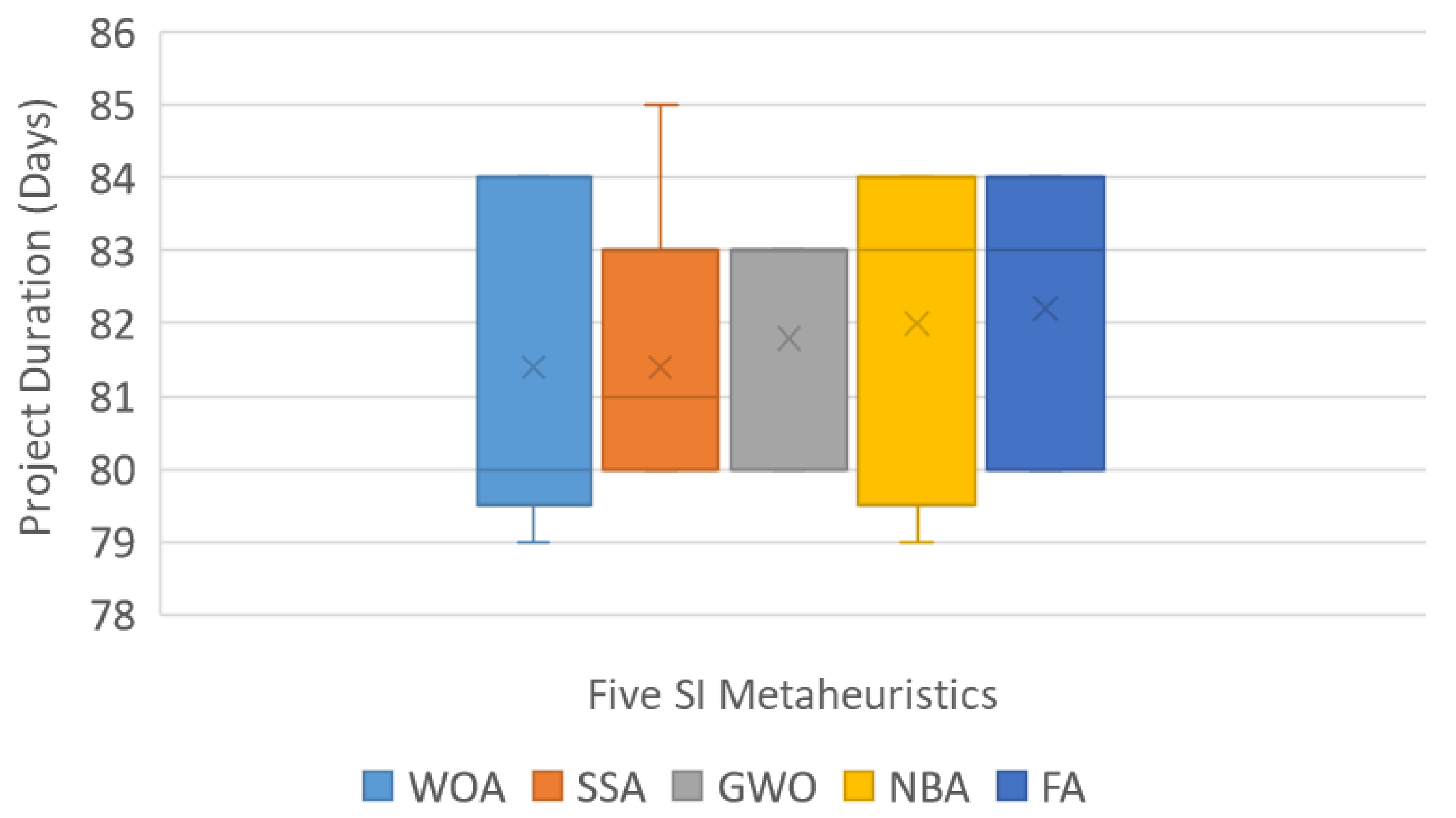
As a new construction method, OSC has the potential to improve the sustainability of the built environment. However, its wider diffusion is hindered by multiple barriers; among them is the need to make extensive planning decisions. This barrier calls for computational methods that help project managers to make the optimum planning decisions. Simulation and optimization are among the key computational methods that can capture the complexity and uncertainty of OSC projects. This study investigated, for the first time, recent SI metaheuristics, namely: the FA, GWO, the NBA, the WOA and the SSA, for the integration of simulation and optimization, and applied them to infrastructure OSC projects to simultaneously minimize projects’ duration and cost.
These SI metaheuristics were applied to a case study of a bridge deck construction project using the OSC method. The construction operations were simulated via a DES model. In order to reduce the computation time of the SO process, CRN and parallel computing were integrated into the SO models, reducing the average computation time by 87.0%. Then, a comparative study based on the convergence behaviour and the statistical analysis of the five SI metaheuristics was conducted. The convergence behaviour analysis indicated that the NBA shows rabid convergence behaviour compared with the other SI metaheuristics. However, GWO shows the best balance between exploration and exploitation to avoid stagnation into local optima. The FA exhibits smooth and steady convergence behaviour, whereas WOA and the SSA suffer from becoming stuck in local points. Based on the 95% confidence level, the statistical analysis proved that there is no statistically significant difference between the solution qualities obtained by GWO, the NBA and the WOA. However, the FA and SSA provide less optimal solutions. This comparative analysis proves that the NBA and GWO are very competitive for the SO of OSC projects. Considering the time and effort needed to tune the controllable parameters of the SI metaheuristics, GWO is preferable to the NBA, because GWO has a smaller number of tuning parameters. Besides this, its simplicity makes it more accessible for researchers to modify its logic or hybridize it with other local search methods to further improve its performance. To summarize, this study contributes to the body of knowledge by comparing multiple and recent SI metaheuristics for the stochastic SO of TCTP in infrastructure OSC projects. Furthermore, the study incorporates CRN and parallel computing with the SO models to reduce the computation time. To the best of the authors’ knowledge, this study is one of the first to integrate recent SI metaheuristics such as the FA, GWO, NBA, WOA and SSA with DES for the SO of OSC projects.
This study offers a valuable reference to professionals and academics who are interested in the optimization of the planning of OSC projects. The integration of CRN and parallel computing with the most recent and powerful SI metaheuristics such as GWO, the NBA and the WOA can provide project managers with near-optimum resource planning and logistics decisions to reap the full sustainability merits of OSC. This study could be seen as one of the early attempts to evaluate the performance of multiple SI metaheuristics in the solution of a set of optimization problems characterized by uncertainty in the construction industry [26]. Hence, it can guide researchers to test the performance of other metaheuristics for the SO of different construction projects.
Nonetheless, this study’s conclusions should be interpreted in the light of some limitations. According to the no-free-lunch theorem, the reported results herein cannot be generalized to other types of construction projects. Furthermore, the developed simulation model ignores some non-physical aspects of OSC projects, such as organizational policies, rework, and the laborers’ skill level. These aspects could be considered using SD, forming a hybrid DES–SD model. Such hybrid models could provide another challenging testbed for SI metaheuristics to optimize real-world systems characterized by complexity and uncertainty. Given the potential and simplicity of GWO in SO for OSC, its performance could be further improved by hybridizing it with local search methods such as the Hooke–Jeeves method and the Nelder–Mead simplex method. Furthermore, different kinds of OSC projects could be used to test SI metaheuristics.

Supplementary Materials

The following are available online at https://0-www-mdpi-com.brum.beds.ac.uk/article/10.3390/su132413551/s1, Table S1: The cost input parameters of the proposed model. Table S2: Overtime policies.

Author Contributions

Conceptualization, A.E.; methodology, M.H. and A.E.E.E.; software, M.H.; validation, A.D., A.E.E.E. and A.E.; formal analysis, M.H.; investigation, M.H., A.D., A.E.E.E. and A.E.; resources, M.H. and A.E.; data curation, M.H. and A.E.E.E.; writing—original draft preparation, M.H.; writing—review and editing, A.D., A.E.E.E. and A.E.; visualization, M.H. and A.E.E.E.; supervision, A.D., A.E.E.E. and A.E.; project administration, A.E.; funding acquisition, A.D. and A.E. All authors have read and agreed to the published version of the manuscript.

Funding

The Egyptian Ministry of Higher Education (MOHE) grant and the Japanese International Cooperation Agency (JICA) in the scope of the Egypt–Japan University of Science and Technology (E-JUST) sponsored this research.

Institutional Review Board Statement

Not applicable.

Informed Consent Statement

Not applicable.

Data Availability Statement

Some or all of the data, models, or code that support this study’s findings are available from the corresponding author upon reasonable request.

Conflicts of Interest

The authors declare there are no competing interests.

References

  1. Hussein, M.; Zayed, T. Critical factors for successful implementation of just-in-time concept in modular integrated construction: A systematic review and meta-analysis. J. Clean. Prod. 2021, 284, 124716. [Google Scholar] [CrossRef] [PubMed]
  2. Hosseini, M.R.; Martek, I.; Zavadskas, E.K.; Aibinu, A.A.; Arashpour, M.; Chileshe, N. Critical evaluation of off-site construction research: A Scientometric analysis. Autom. Constr. 2018, 87, 235–247. [Google Scholar] [CrossRef]
  3. Nam, S.; Yoon, J.; Kim, K.; Choi, B. Optimization of Prefabricated Components in Housing Modular Construction. Sustainability 2020, 12, 10269. [Google Scholar] [CrossRef]
  4. Chen, W.; Zhao, Y.; Yu, Y.; Chen, K.; Arashpour, M. Collaborative Scheduling of On-Site and Off-Site Operations in Prefabrication. Sustainability 2020, 12, 9266. [Google Scholar] [CrossRef]
  5. Wai, C.T.; Yi, P.W.; Olanrewaju, O.I.; Abdelmageed, S.; Hussein, M.; Tariq, S.; Zayed, T. A critical analysis of benefits and challenges of implementing modular integrated construction. Int. J. Constr. Manag. 2021, 1–24. [Google Scholar] [CrossRef]
  6. Kong, L.; Li, H.; Luo, H.; Ding, L.; Zhang, X. Sustainable performance of just-in-time (JIT) management in time-dependent batch delivery scheduling of precast construction. J. Clean. Prod. 2018, 193, 684–701. [Google Scholar] [CrossRef]
  7. Kamali, M.; Hewage, K. Life cycle performance of modular buildings: A critical review. Renew. Sustain. Energy Rev. 2016, 62, 1171–1183. [Google Scholar] [CrossRef]
  8. Hill, C. Prefabrication, and Modularization: Increasing Productivity in the Construction Industry Smart Market Report; McGraw Hill Construction: New York, NY, USA, 2011. [Google Scholar]
  9. Xu, Z.; Zayed, T.; Niu, Y. Comparative analysis of modular construction practices in mainland China, Hong Kong and Singapore. J. Clean. Prod. 2020, 245, 118861. [Google Scholar] [CrossRef]
  10. Salimi, S.; Mawlana, M.; Hammad, A. Performance analysis of simulation-based optimization of construction projects using High Performance Computing. Autom. Constr. 2018, 87, 158–172. [Google Scholar] [CrossRef]
  11. Jiang, W.; Wu, L. Flow shop optimization of hybrid make-to-order and make-to-stock in precast concrete component production. J. Clean. Prod. 2021, 297, 126708. [Google Scholar] [CrossRef]
  12. Wuni, I.Y.; Shen, G.Q. Barriers to the adoption of modular integrated construction: Systematic review and meta-analysis, integrated conceptual framework, and strategies. J. Clean. Prod. 2020, 249, 119347. [Google Scholar] [CrossRef]
  13. Darko, A.; Chan, A.P.; Yang, Y.; Tetteh, M.O. Building information modeling (BIM)-based modular integrated construction risk management—Critical survey and future needs. Comput. Ind. 2020, 123, 103327. [Google Scholar] [CrossRef]
  14. Hussein, M.; Eltoukhy, A.E.; Karam, A.; Shaban, I.A.; Zayed, T. Modelling in off-site construction supply chain management: A review and future directions for sustainable modular integrated construction. J. Clean. Prod. 2021, 310, 127503. [Google Scholar] [CrossRef]
  15. Feng, C.-W.; Liu, L.; Burns, S. Stochastic Construction Time-Cost Trade-Off Analysis. J. Comput. Civ. Eng. 2000, 14, 117–126. [Google Scholar] [CrossRef] [Green Version]
  16. Issa, U.H.; Eid, M.A. An application of genetic algorithms to time-cost-quality trade-off in construction industry. Civ. Environ. Res. 2013, 3, 11–19. Available online: https://www.iiste.org/Journals/index.php/CER/article/view/8635#google_vignette (accessed on 7 December 2021).
  17. Zhang, Y.; Ng, S.T. An ant colony system based decision support system for construction time-cost optimization. J. Civ. Eng. Manag. 2012, 18, 580–589. [Google Scholar] [CrossRef]
  18. Yang, Q. Application of Time-Cost-Quality Tradeoff Optimization Model Based on Improved PSO Algorithm to Construction Project. In Proceedings of the 2009 Asia-Pacific Conference on Information Processing, Shenzhen, China, 18–19 July 2009; IEEE: Washington, DC, USA, 2009; Volume 2, pp. 298–301. [Google Scholar]
  19. De, P.; Dunne, E.J.; Ghosh, J.B.; Wells, C.E. The discrete time-cost tradeoff problem revisited. Eur. J. Oper. Res. 1995, 81, 225–238. [Google Scholar] [CrossRef]
  20. Aladini, K.; Afshar, A.; Kalhor, E. Discounted cash flow time-cost trade-off problem optimization, aco approach. Asian J. Civ Eng. Build. Hous. 2011, 12, 511–522. Available online: https://www.sid.ir/en/journal/ViewPaper.aspx?ID=248038 (accessed on 7 December 2021).
  21. Zareei, M.; Hassan-Pour, H.A. A multi-objective resource-constrained optimization of time-cost trade-off problems in scheduling project. Iran. J. Manag. Stud. 2015, 8, 653–685. [Google Scholar]
  22. Liu, Y.; Dong, J.; Shen, L. A Conceptual Development Framework for Prefabricated Construction Supply Chain Management: An Integrated Overview. Sustainability 2020, 12, 1878. [Google Scholar] [CrossRef] [Green Version]
  23. Borshchev, A. The Big Book of Simulation Modeling: Multimethod modeling with AnyLogic 6; AnyLogic North America: Oakbrook Terrace, IL, USA, 2013; ISBN 0989573176. [Google Scholar]
  24. Kim, T.; Kim, Y.-W.; Cho, H. Dynamic production scheduling model under due date uncertainty in precast concrete construction. J. Clean. Prod. 2020, 257, 120527. [Google Scholar] [CrossRef]
  25. Swisher, J.; Hyden, P.; Jacobson, S.; Schruben, L. A survey of simulation optimization techniques and procedures. In Proceedings of the 2000 Winter Simulation Conference Proceedings (Cat. No.00CH37165), Orlando, FL, USA, 10–13 December 2000; IEEE: Washington, DC, USA, 2000; Volume 1, pp. 119–128. [Google Scholar] [CrossRef]
  26. Juan, A.; Faulin, J.; Grasman, S.E.; Rabe, M.; Figueira, G. A review of simheuristics: Extending metaheuristics to deal with stochastic combinatorial optimization problems. Oper. Res. Perspect. 2015, 2, 62–72. [Google Scholar] [CrossRef] [Green Version]
  27. Mirjalili, S.; Lewis, A. The Whale Optimization Algorithm. Adv. Eng. Softw. 2016, 95, 51–67. [Google Scholar] [CrossRef]
  28. Cheng, T.-M.; Feng, C.-W.; Chen, Y.-L. A hybrid mechanism for optimizing construction simulation models. Autom. Constr. 2005, 14, 85–98. [Google Scholar] [CrossRef]
  29. Marzouk, M.; Moselhi, O. Multiobjective Optimization of Earthmoving Operations. J. Constr. Eng. Manag. 2004, 130, 105–113. [Google Scholar] [CrossRef]
  30. Cheng, T.-M.; Feng, C.-W.; Hsu, M.-Y. An integrated modeling mechanism for optimizing the simulation model of the construction operation. Autom. Constr. 2006, 15, 327–340. [Google Scholar] [CrossRef]
  31. Marzouk, M.M.; Omar, O.A.; Hamid, M.S.A.; El-Said, M.E. An optimization algorithm for simulation-based planning of low-income housing projects. J. Adv. Res. 2010, 1, 291–300. [Google Scholar] [CrossRef] [Green Version]
  32. Mawlana, M.; Hammad, A. Integrating Variance Reduction Techniques and Parallel Computing in Construction Simulation Optimization. J. Comput. Civ. Eng. 2019, 33, 04019026. [Google Scholar] [CrossRef]
  33. Mirjalili, S.; Mirjalili, S.M.; Lewis, A. Grey Wolf Optimizer. Adv. Eng. Softw. 2014, 69, 46–61. [Google Scholar] [CrossRef] [Green Version]
  34. Zhang, H.; Tam, C.M.; Li, H.; Shi, J.J. Particle Swarm Optimization-Supported Simulation for Construction Operations. J. Constr. Eng. Manag. 2006, 132, 1267–1274. [Google Scholar] [CrossRef]
  35. Marzouk, M.; Said, H.; El-Said, M. Framework for Multiobjective Optimization of Launching Girder Bridges. J. Constr. Eng. Manag. 2009, 135, 791–800. [Google Scholar] [CrossRef]
  36. Nassar, K.; El Masry, M.; Sherif, Y. Multiobjective Optimization of Advanced Shoring Systems Used in Bridge Construction. In Computing in Civil Engineering (2011); American Society of Civil Engineers (ASCE): Reston, VA, USA, 2011; pp. 94–101. [Google Scholar]
  37. Mubarak, H.; Mansor, N.; Mokhlis, H.; Mohamad, M.; Mohamad, H.; Muhammad, M.; Al Samman, M.; Afzal, S. Optimum Distribution System Expansion Planning Incorporating DG Based on N-1 Criterion for Sustainable System. Sustainability 2021, 13, 6708. [Google Scholar] [CrossRef]
  38. Alali, M.; Shahooei, Z.; Bahramipanah, M. Resiliency-Oriented Optimization of Critical Parameters in Multi Inverter-Fed Distributed Generation Systems. Sustainability 2021, 13, 6699. [Google Scholar] [CrossRef]
  39. Shabbir, M.; Siddiqi, A.; Yapanto, L.; Tonkov, E.; Poltarykhin, A.; Pilyugina, A.; Petrov, A.; Foroughi, A.; Valiullina, D. Closed-Loop Supply Chain Design and Pricing in Competitive Conditions by Considering the Variable Value of Return Products Using the Whale Optimization Algorithm. Sustainability 2021, 13, 6663. [Google Scholar] [CrossRef]
  40. Qais, M.H.; Hasanien, H.M.; Alghuwainem, S. Enhanced salp swarm algorithm: Application to variable speed wind generators. Eng. Appl. Artif. Intell. 2019, 80, 82–96. [Google Scholar] [CrossRef]
  41. Sörensen, K. Metaheuristics-the metaphor exposed. Int. Trans. Oper. Res. 2015, 22, 3–18. [Google Scholar] [CrossRef]
  42. Hussein, M.; Zayed, T. Crane operations and planning in modular integrated construction: Mixed review of literature. Autom. Constr. 2021, 122, 103466. [Google Scholar] [CrossRef]
  43. Karam, A.; Hussein, M.; Reinau, K.H. Analysis of the barriers to implementing horizontal collaborative transport using a hybrid fuzzy Delphi-AHP approach. J. Clean. Prod. 2021, 321, 128943. [Google Scholar] [CrossRef]
  44. Tariq, S.; Hussein, M.; Wang, R.D.; Zayed, T. Trends and developments of on-site crane layout planning 1983–2020: Bibliometric, scientometric and qualitative analyses. Constr. Innov. 2021. [Google Scholar] [CrossRef]
  45. Moher, D.; Liberati, A.; Tetzlaff, J.; Altman, D.G.; The PRISMA Group. Preferred reporting items for systematic reviews and meta-analyses: The PRISMA Statement. PLoS Med. 2009, 6, e1000097-6. [Google Scholar] [CrossRef] [Green Version]
  46. Alzraiee, H.; Zayed, T.; Moselhi, O. Dynamic planning of construction activities using hybrid simulation. Autom. Constr. 2015, 49, 176–192. [Google Scholar] [CrossRef]
  47. Shitole, V.; Louis, J.; Tadepalli, P. Optimizing Earth Moving Operations Via Reinforcement Learning. In Proceedings of the 2019 Winter Simulation Conference (WSC), National Harbor, MD, USA, 8–12 December 2019; IEEE: Washington, DC, USA, 2019; pp. 2954–2965. [Google Scholar]
  48. Li, H.X.; Zhang, L.; Mah, D.; Yu, H. An integrated simulation and optimization approach for reducing CO 2 emissions from on-site construction process in cold regions. Energy Build. 2017, 138, 666–675. [Google Scholar] [CrossRef]
  49. Altaf, M.S.; Bouferguene, A.; Liu, H.; Al-Hussein, M.; Yu, H. Integrated production planning and control system for a panelized home prefabrication facility using simulation and RFID. Autom. Constr. 2018, 85, 369–383. [Google Scholar] [CrossRef]
  50. Chen, S.; Feng, K.; Lu, W. A Simulation-Based Optimisation for Contractors in Precast Concrete Projects. In 10th Nordic Conference on Construction Economics and Organization, Tallinn, Estonia, 7–8 May 2019; Lill, I., Witt, E., Eds.; Emerald Publishing Limited: Bingley, UK, 2019; Volume 2, pp. 137–145. [Google Scholar]
  51. Lamas-Rodríguez, A.; Pernas-Álvarez, J.; Taracido-López, I. Constrained-based discrete-event simulation of an assembly job shop in the offshore wind industry. In Proceedings of the 32nd European Modeling & Simulation Symposium (EMSS 2020), online, 16–18 September 2020; Cal-Tek Srl: Cosenza, Italy, 2020; pp. 62–91. [Google Scholar] [CrossRef]
  52. Robertson, B.; Srinivasan, R.; McFarlane, D. Dynamic Postponement in Off-Site/On-Site Construction Operations in the Face of On-Site Disruptions; Springer International Publishing: Cham, Switzerland, 2018; pp. 261–272. [Google Scholar] [CrossRef]
  53. Taghaddos, H.; Hermann, U.; Abourizk, S.; Mohamed, Y. Simulation-Based Scheduling of Modular Construction Using Multi-Agent Resource Allocation. In Proceedings of the 2010 Second International Conference on Advances in System Simulation, Nice, France, 22–27 August 2010; IEEE: Washington, DC, USA, 2010; pp. 115–120. [Google Scholar] [CrossRef]
  54. Altaf, M.S.; Al-Hussein, M.; Yu, H. Wood-Frame Wall Panel Sequencing Based on Discrete-Event Simulation and Particle Swarm Optimization. In Proceedings of the Proceedings of the 31st International Symposium on Automation and Robotics in Construction and Mining (ISARC), Sydney, Australia, 9–11 July 2014; International Association for Automation and Robotics in Construction (IAARC): Bratislava, Slovakia, 2014; pp. 254–261. [Google Scholar] [CrossRef] [Green Version]
  55. Yusuf, M.; Karam, A.; Eltawil, A. A Simulation based Optimization Study for Optimum Sequencing of Precast Components Considering Supply Chain Risks. In Proceedings of the 8th International Conference on Operations Research and Enterprise Systems, Prague, Czech Republic, 19–21 February 2019; SciTePress: Setúbal, Portugal, 2019; pp. 330–337. [Google Scholar] [CrossRef]
  56. Yusuf, M.; Karam, A.; Eltawil, A. A Stochastic Optimization Approach of Flow Shop Sequencing Problem for On-time Delivery of Precast Components. In Proceedings of the 8th International Conference on Operations Research and Enterprise Systems, Prague, Czech Republic, 19–21 February 2019; SciTePress: Setúbal, Portugal, 2019; pp. 245–252. [Google Scholar] [CrossRef]
  57. Wang, Z.; Hu, H.; Gong, J. Framework for modeling operational uncertainty to optimize offsite production scheduling of precast components. Autom. Constr. 2018, 86, 69–80. [Google Scholar] [CrossRef]
  58. Taghaddos, H.; Eslami, A.; Hermann, U.; AbouRizk, S.; Mohamed, Y. Auction-based Simulation for Industrial Crane Operations. Autom. Constr. 2019, 104, 107–119. [Google Scholar] [CrossRef]
  59. Cheng, T.-M.; Yan, R.-Z. Integrating Messy Genetic Algorithms and Simulation to Optimize Resource Utilization. Comput. Civ. Infrastruct. Eng. 2009, 24, 401–415. [Google Scholar] [CrossRef]
  60. Liu, Y.; Mohamed, Y. Modelling industrial construction operations using a multi-agent resource allocation framework. Eng. Constr. Arch. Manag. 2012, 19, 406–427. [Google Scholar] [CrossRef]
  61. Yazdani, M.; Kabirifar, K.; Fathollahi-Fard, A.M.; Mojtahedi, M. Production scheduling of off-site prefabricated construction components considering sequence dependent due dates. Environ. Sci. Pollut. Res. 2021, 1–17. [Google Scholar] [CrossRef] [PubMed]
  62. Lin, C.-T.; Hsie, M.; Hsiao, W.-T.; Wu, H.-T.; Cheng, T.-M. Optimizing the Schedule of Dispatching Earthmoving Trucks through Genetic Algorithms and Simulation. J. Perform. Constr. Facil. 2012, 26, 203–211. [Google Scholar] [CrossRef] [Green Version]
  63. Cheng, M.-Y.; Tran, D.-H. Integrating Chaotic Initialized Opposition Multiple-Objective Differential Evolution and Stochastic Simulation to Optimize Ready-Mixed Concrete Truck Dispatch Schedule. J. Manag. Eng. 2016, 32, 04015034. [Google Scholar] [CrossRef]
  64. Zhou, F.; Abourizk, S.M.; AL-Battaineh, H. Optimisation of construction site layout using a hybrid simulation-based system. Simul. Model. Pract. Theory 2009, 17, 348–363. [Google Scholar] [CrossRef]
  65. Zhang, H.; Li, H. Simulation-based optimization for dynamic resource allocation. Autom. Constr. 2004, 13, 409–420. [Google Scholar] [CrossRef]
  66. Lu, M.; Lam, H.-C.; Dai, F. Resource-constrained critical path analysis based on discrete event simulation and particle swarm optimization. Autom. Constr. 2008, 17, 670–681. [Google Scholar] [CrossRef]
  67. Shin, Y.; Cho, H.; Kang, K.-I. Simulation model incorporating genetic algorithms for optimal temporary hoist planning in high-rise building construction. Autom. Constr. 2011, 20, 550–558. [Google Scholar] [CrossRef]
  68. Fayed, R.A.; Ezeldin, A.S. Simulation and optimization model for electrical substation construction. J. Inf Technol. Constr. 2018, 23, 215. [Google Scholar]
  69. Szczesny, K.; Hamm, M.; König, M. Adjusted recombination operator for simulation-based construction schedule optimization. In Proceedings of the 2012 Winter Simulation Conference (WSC), Berlin, Germany, 9–12 December 2012; IEEE: Washington, DC, USA, 2012; pp. 1–10. [Google Scholar]
  70. Cao, M.; Lu, M.; Zhang, J.-P. Concrete plant operations optimization using combined simulation and genetic algorithms. In Proceedings of the 2004 International Conference on Machine Learning and Cybernetics (IEEE Cat. No.04EX826), Shanghai, China, 26–29 August 2004; IEEE: Washington, DC, USA, 2005; Volume 7, pp. 4204–4209. [Google Scholar]
  71. Zankoul, E.; Khoury, H. Modeling, Animating, and Optimizing On-Shore Wind Farm Construction Operations. J. Comput. Civ. Eng. 2016, 30, 05016001. [Google Scholar] [CrossRef] [Green Version]
  72. Younes, A.; Marzouk, M. Tower cranes layout planning using agent-based simulation considering activity conflicts. Autom. Constr. 2018, 93, 348–360. [Google Scholar] [CrossRef]
  73. Feng, K.; Lu, W.; Chen, S.; Wang, Y. An Integrated Environment–Cost–Time Optimisation Method for Construction Contractors Considering Global Warming. Sustainability 2018, 10, 4207. [Google Scholar] [CrossRef] [Green Version]
  74. Hamm, M.; Szczesny, K.; Nguyen, V.V.; Konig, M. Optimization of Construction Schedules with Discrete-Event Simulation Using an Optimization Framework. In Computing in Civil Engineering (2011); American Society of Civil Engineers (ASCE): Reston, VA, USA, 2011; pp. 682–689. [Google Scholar]
  75. Hsiao, W.-T.; Lin, C.-T.; Wu, H.-T.; Cheng, T.-M. A Hybrid Optimization Mechanism Used to Generate Truck Fleet to Perform Earthmoving Operations. In Instrumentation, Testing, and Modeling of Soil and Rock Behavior; American Society of Civil Engineers (ASCE): Reston, VA, USA, 2011; pp. 151–159. [Google Scholar]
  76. Lu, M.; Dai, F.; Chen, W. Real-time decision support for planning concrete plant operations enabled by integrating vehicle tracking technology, simulation, and optimization algorithms. Can. J. Civ. Eng. 2007, 34, 912–922. [Google Scholar] [CrossRef]
  77. Yu, B.; Meng, X.; Liu, Q. Multi-objective optimisation of hot in-place recycling of asphalt pavement considering environmental impact, cost and construction quality. Int. J. Pavement Eng. 2020, 21, 1576–1584. [Google Scholar] [CrossRef]
  78. Szczesny, K.; König, M. Reactive scheduling based on actual logistics data by applying simulation-based optimization. Vis. Eng. 2015, 3, 10. [Google Scholar] [CrossRef] [Green Version]
  79. Dashti, M.S.; RezaZadeh, M.; Khanzadi, M.; Taghaddos, H. Integrated BIM-based simulation for automated time-space conflict management in construction projects. Autom. Constr. 2021, 132, 103957. [Google Scholar] [CrossRef]
  80. Yazdani, M.; Kabirifar, K.; Frimpong, B.E.; Shariati, M.; Mirmozaffari, M.; Boskabadi, A. Improving construction and demolition waste collection service in an urban area using a simheuristic approach: A case study in Sydney, Australia. J. Clean. Prod. 2021, 280, 124138. [Google Scholar] [CrossRef]
  81. Nadoushani, Z.S.M.; Nezhad, A.A.; Rey, D. Optimization of concrete placing operation based on competing carbon footprint, cost and production rate objectives. Eng. Constr. Arch. Manag. 2018, 25, 938–957. [Google Scholar] [CrossRef]
  82. Marzouk, M.; Azab, S.; Metawie, M. Framework for Sustainable Low-Income Housing Projects using Building Information Modeling. J. Environ. Inform. 2016, 28, 1–25. [Google Scholar] [CrossRef] [Green Version]
  83. Beißert, U.; König, M.; Bargstädt, H.-J. Soft Constraint-based simulation of execution strategies in building engineering. J. Simul. 2010, 4, 222–231. [Google Scholar] [CrossRef]
  84. Zhang, J.; Zhang, Y.; Hu, Z.; Lu, M. Construction management utilizing 4D CAD and operations simulation methodologies. Tsinghua Sci. Technol. 2008, 13, 241–247. [Google Scholar] [CrossRef]
  85. Zivkovic, M.; Bacanin, N.; Venkatachalam, K.; Nayyar, A.; Djordjevic, A.; Strumberger, I.; Al-Turjman, F. COVID-19 cases prediction by using hybrid machine learning and beetle antennae search approach. Sustain. Cities Soc. 2021, 66, 102669. [Google Scholar] [CrossRef] [PubMed]
  86. Feng, K.; Chen, S.; Lu, W. Machine learning based construction simulation and optimization. In Proceedings of the 2018 Winter Simulation Conference (WSC), Gothenburg, Sweden, 9–12 December 2018; IEEE: Washington, DC, USA, 2018; pp. 2025–2036. [Google Scholar]
  87. Dorrah, D.H.; Marzouk, M. Integrated multi-objective optimization and agent-based building occupancy modeling for space layout planning. J. Build. Eng. 2021, 34, 101902. [Google Scholar] [CrossRef]
  88. Elbeltagi, E.; Hegazy, T.; Grierson, D. Comparison among five evolutionary-based optimization algorithms. Adv. Eng. Inform. 2005, 19, 43–53. [Google Scholar] [CrossRef]
  89. Elbehairy, H.; Elbeltagi, E.; Hegazy, T.; Soudki, K. Comparison of Two Evolutionary Algorithms for Optimization of Bridge Deck Repairs. Comput. Civ. Infrastruct. Eng. 2006, 21, 561–572. [Google Scholar] [CrossRef]
  90. El-Ghandour, H.A.; Elbeltagi, E. Comparison of Five Evolutionary Algorithms for Optimization of Water Distribution Networks. J. Comput. Civ. Eng. 2018, 32, 04017066. [Google Scholar] [CrossRef]
  91. Gandomi, A.H.; Kashani, A.R. Construction Cost Minimization of Shallow Foundation Using Recent Swarm Intelligence Techniques. IEEE Trans. Ind. Inform. 2017, 14, 1099–1106. [Google Scholar] [CrossRef]
  92. Kaveh, A.; Seddighian, M.R. Domain decomposition of finite element models utilizing eight meta-heuristic algorithms: A comparative study. Mech. Based Des. Struct. Mach. 2020, 1–19. [Google Scholar] [CrossRef]
  93. Goodarzian, F.; Hosseini-Nasab, H.; Muñuzuri, J.; Fakhrzad, M.-B. A multi-objective pharmaceutical supply chain network based on a robust fuzzy model: A comparison of meta-heuristics. Appl. Soft Comput. 2020, 92, 106331. [Google Scholar] [CrossRef]
  94. Eltoukhy, A.E.; Chan, F.T.; Chung, S.H.; Niu, B.; Wang, X. Heuristic approaches for operational aircraft maintenance routing problem with maximum flying hours and man-power availability considerations. Ind. Manag. Data Syst. 2017, 117, 2142–2170. [Google Scholar] [CrossRef]
  95. Kaveh, A.; Hamedani, K.B.; Hosseini, S.M.; Bakhshpoori, T. Optimal design of planar steel frame structures utilizing meta-heuristic optimization algorithms. Structures 2020, 25, 335–346. [Google Scholar] [CrossRef]
  96. Alberdi, R.; Khandelwal, K. Comparison of robustness of metaheuristic algorithms for steel frame optimization. Eng. Struct. 2015, 102, 40–60. [Google Scholar] [CrossRef]
  97. Mostafa, S.; Kim, K.P.; Tam, V.W.Y.; Rahnamayiezekavat, P. Exploring the status, benefits, barriers and opportunities of using BIM for advancing prefabrication practice. Int. J. Constr. Manag. 2020, 20, 146–156. [Google Scholar] [CrossRef]
  98. Marler, R.T.; Arora, J.S. Function-transformation methods for multi-objective optimization. Eng. Optim. 2005, 37, 551–570. [Google Scholar] [CrossRef]
  99. Luo, H.; Liu, J.; Li, C.; Chen, K.; Zhang, M. Ultra-rapid delivery of specialty field hospitals to combat COVID-19: Lessons learned from the Leishenshan Hospital project in Wuhan. Autom. Constr. 2020, 119, 103345. [Google Scholar] [CrossRef] [PubMed]
  100. Eltoukhy, A.E.E.; Wang, Z.X.; Chan, F.T.S.; Chung, S.H.; Ma, H.-L.; Wang, X.P. Robust Aircraft Maintenance Routing Problem Using a Turn-Around Time Reduction Approach. IEEE Trans. Syst. Man, Cybern. Syst. 2020, 50, 4919–4932. [Google Scholar] [CrossRef]
  101. Eltoukhy, A.E.; Wang, Z.; Chan, F.T.; Fu, X. Data analytics in managing aircraft routing and maintenance staffing with price competition by a Stackelberg-Nash game model. Transp. Res. Part E Logist. Transp. Rev. 2019, 122, 143–168. [Google Scholar] [CrossRef]
  102. Amaran, S.; Sahinidis, N.V.; Sharda, B.; Bury, S.J. Simulation optimization: A review of algorithms and applications. Ann. Oper. Res. 2016, 240, 351–380. [Google Scholar] [CrossRef] [Green Version]
  103. Tekin, E.; Sabuncuoglu, I. Simulation optimization: A comprehensive review on theory and applications. IIE Trans. 2004, 36, 1067–1081. [Google Scholar] [CrossRef]
  104. Wang, L.-F.; Shi, L.-Y. Simulation Optimization: A Review on Theory and Applications. Acta Autom. Sin. 2013, 39, 1957–1968. [Google Scholar] [CrossRef]
  105. MATLAB. The MathWorks, Inc. 2005. Available online: http://www.mathworks.com (accessed on 7 December 2021).
  106. Yang, X.-S. Firefly Algorithms for Multimodal Optimization. In International Symposium on Stochastic Algorithms; Springer: Berlin/Heidelberg, Germany, 2009; pp. 169–178. [Google Scholar]
  107. Meng, X.-B.; Gao, X.; Liu, Y.; Zhang, H. A novel bat algorithm with habitat selection and Doppler effect in echoes for optimization. Expert Syst. Appl. 2015, 42, 6350–6364. [Google Scholar] [CrossRef]
  108. Zhong, M.; Long, W. Whale optimization algorithm with nonlinear control parameter. In Proceedings of the MATEC Web of Conferences, Chengdu, China, 16–17 December 2017; EDP Sciences: Les Ulis, France, 2017; Volume 139, p. 00157. [Google Scholar] [CrossRef]
  109. Kaveh, A.; Ghazaan, M.I. Enhanced whale optimization algorithm for sizing optimization of skeletal structures. Mech. Based Des. Struct. Mach. 2016, 45, 345–362. [Google Scholar] [CrossRef]
  110. Mirjalili, S.; Gandomi, A.H.; Mirjalili, S.Z.; Saremi, S.; Faris, H.; Mirjalili, S.M. Salp Swarm Algorithm: A bio-inspired optimizer for engineering design problems. Adv. Eng. Softw. 2017, 114, 163–191. [Google Scholar] [CrossRef]
  111. Wang, Q.; Guidolin, M.; Savic, D.; Kapelan, Z. Two-Objective Design of Benchmark Problems of a Water Distribution System via MOEAs: Towards the Best-Known Approximation of the True Pareto Front. J. Water Resour. Plan. Manag. 2015, 141, 04014060. [Google Scholar] [CrossRef] [Green Version]
  112. Stützle, T.; López-Ibáñez, M.; Pellegrini, P.; Maur, M.; de Oca, M.M.; Birattari, M.; Dorigo, M. Parameter Adaptation in Ant Colony Optimization. Auton. Search 2011, 191–215. [Google Scholar] [CrossRef]
  113. Law, A.M.; Kelton, W.D.; Kelton, W.D. Simulation Modeling and Analysis; McGraw-Hill: New York, NY, USA, 2000; Volume 3, ISBN 10: 0073401323. [Google Scholar]
  114. Kelton, W.D.; Sadowski, R.P.; Sturrock, D.T. Simulation with Arena; McGraw-Hill Higher Education: New York, NY, USA, 2003; ISBN 10: 0073401315. [Google Scholar]
  115. Crainic, T. Parallel Metaheuristics and Cooperative Search. In International Series in Operations Research & Management Science; Springer International Publishing: Cham, Switzerland, 2019; pp. 419–451. [Google Scholar]
  116. Barney, B. Introduction to Parallel Computing; Lawrence Livermore National Laboratory: Livermore, CA, USA, 2010; Volume 6, pp. 169–178. Available online: https://hpc.llnl.gov/training/tutorials/introduction-parallel-computing-tutorial (accessed on 7 December 2021).
  117. Gendreau, M.; Potvin, J.-Y. Handbook of Metaheuristics; Springer Science and Business Media LLC: Berlin/Heidelberg, Germany, 2010; Volume 2. [Google Scholar]
  118. Mawlana, M. Improving Stochastic Simulation-based Optimization for Selecting Construction Method of Precast Box Girder Bridges. Ph.D. Thesis, Concordia University, Montreal, Canada, 30 July 2015. Available online: https://spectrum.library.concordia.ca/980234/ (accessed on 7 December 2021).
  119. Abourizk, S.M.; Halpin, D.W. Statistical Properties of Construction Duration Data. J. Constr. Eng. Manag. 1992, 118, 525–544. [Google Scholar] [CrossRef]
  120. McCabe, B. In Construction engineering and project management III: Monte carlo simulation for schedule risks. In Proceedings of the 35th Conference on Winter Simulation: Driving Innovation, New Orleans, LA, USA, 7–10 December 2003; ACM Press: New York, NY, USA, 2003; pp. 1561–1565. [Google Scholar] [CrossRef]
  121. Faghihi, V.; Reinschmidt, K.F.; Kang, J.H. Objective-driven and Pareto Front analysis: Optimizing time, cost, and job-site movements. Autom. Constr. 2016, 69, 79–88. [Google Scholar] [CrossRef]
  122. Wood, D.A. Gas and oil project time-cost-quality tradeoff: Integrated stochastic and fuzzy multi-objective optimization applying a memetic, nondominated, sorting algorithm. J. Nat. Gas Sci. Eng. 2017, 45, 143–164. [Google Scholar] [CrossRef]
  123. Zhang, L.; Du, J.; Zhang, S. Solution to the Time-Cost-Quality Trade-off Problem in Construction Projects Based on Immune Genetic Particle Swarm Optimization. J. Manag. Eng. 2014, 30, 163–172. [Google Scholar] [CrossRef]
  124. April, J.; Glover, F.; Kelly, J.; Laguna, M. Simulation/optimization using real-world applications. In Proceeding of the 2001 Winter Simulation Conference (Cat. No.01CH37304), Arlington, VA, USA, 9–12 December 2001; IEEE: Washington, DC, USA, 2002; pp. 134–138. [Google Scholar] [CrossRef]
  125. Montgomery, D.C. Design and Analysis of Experiments; John Wiley & Sons: Hoboken, NJ, USA, 2017; ISBN 978-1-119-49244-3. [Google Scholar]
  126. Zhao, M.; Wang, X.; Yu, J.; Bi, L.; Xiao, Y.; Zhang, J. Optimization of Construction Duration and Schedule Robustness Based on Hybrid Grey Wolf Optimizer with Sine Cosine Algorithm. Energies 2020, 13, 215. [Google Scholar] [CrossRef] [Green Version]
  127. Zhang, J.; Zhong, D.; Zhao, M.; Yu, J.; Lv, F. An Optimization Model for Construction Stage and Zone Plans of Rockfill Dams Based on the Enhanced Whale Optimization Algorithm. Energies 2019, 12, 466. [Google Scholar] [CrossRef] [Green Version]
Figure 1. PRISMA flow diagram for the studies’ screening and selection.
Sustainability 13 13551 g001
Figure 2. Classification of studies on SO in the construction research field. GA, genetic algorithm; PSO, particle swarm optimization; OptQuest, commercial optimization solver; EA, evolutionary algorithm; ACO, ant colony optimization; SA, simulated annealing. (a) Construction applications; (b) optimization dimension; (c) metaheuristics.
Sustainability 13 13551 g002aSustainability 13 13551 g002b
Figure 3. Sequence of activities of precast full-span bridge deck construction using a launching gantry, and its associated resources. NT, number of trailers; NRC, number of rebar cage molds; NIM, number of inner molds; NOM, number of outer molds; NPC, number of preparation crews; NSC, number of pre-stressing crews; NFC, number of reinforcement crews; NCC, number of casting crews; YS, casting yard space; YC, yard crane; LG, launching gantry; TR, trolley; OC, on-site crane.
Sustainability 13 13551 g003
Figure 4. General framework of the adopted simulation optimization approach. DES, Discrete-event simulation.
Sustainability 13 13551 g004
Figure 5. Discrete-event simulation model of a precast full-span construction project using a launching gantry in the MATLAB environment.
Sustainability 13 13551 g005
Figure 6. The pseudo-code of the FA.
Sustainability 13 13551 g006
Figure 7. The pseudo-code of the GWO algorithm.
Sustainability 13 13551 g007
Figure 8. The pseudo-code of the NBA.
Sustainability 13 13551 g008
Figure 9. The pseudo-code of WOA.
Sustainability 13 13551 g009
Figure 10. The pseudo-code of the SSA.
Sustainability 13 13551 g010
Figure 11. The master–slave paradigm for the parallelization of SO.
Sustainability 13 13551 g011
Figure 12. The computation time associated with a different number of cores for the parallelization of metaheuristics.
Sustainability 13 13551 g012
Figure 13. The convergence curves of the five SI metaheuristics.
Sustainability 13 13551 g013
Figure 14. Box and whisker plot of the near-optimum project durations obtained by the five SI metaheuristics.
Sustainability 13 13551 g014
Figure 15. Box and whisker plot of the near-optimum project costs obtained by the five SI metaheuristics (USD, United States Dollars).
Sustainability 13 13551 g015
Figure 16. Box and whisker plot of the near-optimum fitness values of the solutions obtained by the five SI metaheuristics.
Sustainability 13 13551 g016
Figure 17. Tukey pairwise comparisons between the five SI metaheuristics conducted by Minitab 18 software.
Sustainability 13 13551 g017
Table 1. Summary of the previous studies on SO in the construction research field.
Construction MethodConstruction ApplicationObjective FunctionSim. MMetaheuristicSingle ObjectiveMulti-ObjectiveParallel ComputingVRT *Reference
OSCOnsite panelized construction Minimize CO2 emissions from the on-site constructionDESGA [48]
Production planning in Panelized constructionMinimize the production timeDESPSO and SA [49]
Planning of precast supply chain and construction configuration Minimize project duration, costs and GHG emissions DESPSO [50]
Job shop scheduling for construction of off-shore wind foundationMinimize total tardiness and maximize total earlinessDESOptQuest (scatter search) [51]
Disruption management of OSC supply chainMinimize total costsDESGA [52]
Project scheduling and resource allocation in modular construction Maximize welfare of stakeholdersDESHeuristics (greedy and ascending-auctionalgorithm) [53]
Production sequencing in wood Panelized constructionMinimize the makespanDESPSO [54]
Production planning of precast componentsMinimizeunit cost or maximize production rateDESGA [30]
Planning of Precast beam bridge deck construction using launching gantryMinimize project duration and costsDESACO [35]
Planning of Housing construction using precast componentsMinimize project duration and costsDESGA [31]
Production planning of precast components Achieve On-time delivery and minimize production costsDESOptQuest [55,56]
Planning of Precast full-span bridge deck construction using launching gantryMinimize project duration and costsDESNSGA-II [10]
Planning of Precast full-span bridge deck construction using launching gantryMinimize project duration and costsDESfmGA [32]
Production scheduling of precast components Minimize delivery penalty costs DESGA [57] *
Crane operation and planning Maximize the system’s social welfare DESHeuristic (Auction protocol) [58] *
Resource assignment in precast production facilities Maximize the production rate or minimize the system’s unit costDESMessy GA [59]
OSCResource allocation in industrial construction projectsMaximize the system’s social welfareABSHeuristics (Greedy and dynamic programming algorithms) [60]
Production scheduling of precast components Minimize inventory costs and delivery penalty costs DESGA, DE, and ICA [61]
Traditional constructionEarthmoving operationsMinimize time and cost of earthmoving operations.DESGA [29]
Fleet management of earth moving trucksMinimize the time of earthmoving operations.DESGA [62]
Dispatch scheduling of concrete batch plants. Minimize the idle time of trucks and construction sites. DESDE [63]
Tunnel construction site layoutMinimize site layout costsDESGA [64]
Resource allocation for bridge construction Minimize project durationDESHeuristic [65]
Activity scheduling and resource allocation Minimize project durationDESPSO [66]
Temporary hoist planning in high-rise building constructionMinimize the hoists’ rental costs DESGA [67]
Construction of electrical substationsMinimize project durationDESGA [68]
Scheduling of shell construction projectMinimize project durationDESEA [69]
Concrete plant operationMinimize site idle time and maximize plant utilization DESGA [70]
On-shore wind farm construction planningMinimize total construction costsDESOptQuest [71]
Tower crane layout planning Minimize hoisting time or total costs ABSOptQuest [72]
Building construction planningMinimize project duration, costs and environmental impactDESPSO [73]
Scheduling of complex construction Minimize the project duration and maximize resource utilizationsDESNSGA-II [74]
Fleet management of earth moving trucksMinimize the operational timeDESGA [75]
Planning concrete plant operation Minimize total operations inefficiencies DESPSO [76]
Planning of hot in-place recycling of asphalt pavementMinimize cost and environmental impact and maximize qualityDESNSGA-II [77]
Construction scheduling Minimize project delay and resource costsDESNSGA-II [78]
Sewer pipeline installationMaximize system production rate or minimize the unit costDESHybrid heuristic-GA [28]
Traditional constructionPlanning of bridge deck construction using advanced shoring methodMinimize project duration and costsDESPSO [36]
Planning of concrete placement operationMaximize productivityor minimize costDESPSO [34]
Time-space conflictplanningCollision-free shortest path DESRapidly-exploring Random Tree [79]
Route planning for construction waste collectionMinimize travel timeMCGA [80]
Concrete placingoperationMinimize carbon emissions and costs & Maximize the production rate DESFull enumeration [81]
Sustainability of low-income housing projectsMinimize life cycle costs & Maximize LEED creditDES & SDNSGA-II [82] *
Scheduling of execution processes in building projectsMinimize makespanDESGreedyRandomized Adaptive Search Procedure [83]
Site layout planning and resource allocation Minimize the project’s duration DESGA [84]
Sim. M, simulation method; VRT, variance reduction technique; DES, discrete-event simulation; GA, genetic algorithm; PSO, particle swarm optimization; SA, simulated annealing; ACO, ant colony optimization; NSGA-II, non-dominated sorting genetic algorithm II; fmGA, fast messy genetic algorithm; EA, evolutionary algorithm ABS, Agent-based simulation; DE, differential evolution; ICA, imperialist competitive algorithm; MC, Monte Carlo simulation; SD, system dynamics. * Sequential simulation-based optimization.
Table 2. The indices, parameters and decision variables used in the optimization model.
Indicies
Prefabricated box girders; g   G , G is the set of girders.
p Production processes; p P , P is the set of production processes.
l Logistics processes; l L , L is the set of logistics processes.
i Installation processes; i I , I is the set of installation processes.
e Equipment resources; e E , E is the set of equipment.
c Human resources (i.e., crews); c C , C is the set of crews.
Parameters
T g p Duration spent by a girder g in a production process p .
T g l Duration spent by a girder g in a logistics process l .
T g i Duration spent by a girder g in an installation process i .
W g p Time waited by a girder g for a production process p .
W g l Time waited by a girder g for a logistics process l .
W g i Time waited by a girder g for an installation process i .
C I C Daily indirect or overhead costs.
M C E p e Mobilization cost of an equipment e used in a production process p .
M C E l e Mobilization cost of an equipment e used in a logistics process l .
M C E i e Mobilization cost of an equipment e used in an installation process i .
M C C p c Mobilization cost of a crew c working on a production process p .
M C C l c Mobilization cost of a crew c working on a logistics process l .
M C C i c Mobilization cost of a crew c working on an installation process i .
F C p e Fixed cost of an equipment e used in a production process p .
R E p e Hourly cost of an equipment e used in a production process p .
R E l e Hourly cost of an equipment e used in a logistics process l .
R E i e Hourly cost of an equipment e used in an installation process i .
T E p e Duration spent by an equipment e working on production processes P .
T E l e Duration spent by an equipment e working on logistics processes   L .
T E i e Duration spent by an equipment e working on installation processes I .
R C p c Hourly cost of crew c working on a production process p .
R C l c Hourly cost of crew c working on a logistics process l .
  R C i c Hourly cost of crew c working on an installation process i .
T C p c Duration spent by crew c working on production processes P .
T C l c Duration spent by crew c working on logistics processes   L .
T C i c Duration spent by crew c working on installation processes I .
ϕ p c Overtime cost adjustment factor of crew c working on production processes P .
ϕ l c Overtime cost adjustment factor of crew c working on logistics processes   L .
ϕ i c Overtime cost adjustment factor of crew c working on installation processes I .
C S Hourly storage cost.
n e p e ,   n e l e , and n e i e The maximum number of equipment e available for production p , logistics l , and installation i processes, respectively.
n c p c ,   n c l c , and n c i c The maximum number of crew c available for production p , logistics l , and installation i processes, respectively.
P Y D m i n   and   P Y D m a x The minimum and maximum distances between the construction site and available locations for the production facility.
Y S m i n   and   Y S m a x The minimum and maximum storage capacity of the production yard.
S T m i n   and   S T m a x The minimum and maximum storage time of girders at the production yard.
D W H m i n   and   D W H m a x The minimum and maximum number of daily working hours.
W W D m i n   and   W W D m a x The minimum and maximum number of working days per week.
Decision variables
D W H Number of daily working hours.
W W D Number of working days per week.
N E p e Number of equipment resource e used in a production process p .
N E l e Number of equipment resource e used in a logistics process l .
N E i e Number of equipment resource e used in an installation process i .
N C p c Number of crew c working in a production process p .
N C l c Number of crew c working in a logistics process l .
N C i c Number of crew c working in an installation process i .
Y S Storage capacity of the production yard.
S T Storage time of girders at the production yard.
P Y D The distance between the construction site and available locations to set up the production yard.
Table 3. The methods used to tune the parameters’ values of each SI metaheuristic.
MetaheuristicParameterParameter Tuning MethodValue or Range
FAlight absorption coefficient γ Self-adaptive(1–30)
constant number α Self-adaptive(0.1–0.2)
GWOParameter a Pre-scheduled (2–0)
Coefficient C Pre-scheduled (0–2)
NBAConstant α Offline (constant) 0.99
Constant γ Offline (constant)0.9
Probability of habitat selection P Pre-scheduled
(random number within the range)
(0.6–0.9)
Frequency of updating loudness and pulse emission rate G Offline (constant)4
Compensation rate for Doppler effect in echoes C Pre-scheduled
(random number within the range)
(0.1–0.9)
Inertia weight   w Pre-scheduled (0.5–0.9)
Contraction–expansion coefficient θ Pre-scheduled (0.5–1)
WOAParameter a Pre-scheduled (2–0)
positive number to define the spiral shape b Self-adaptive(0.5–2)
SSAParameter C 1 Pre-scheduled (2–0)
Table 4. The two solutions used to check the efficacy of the use of CRN.
Decision VariablesSolutions
AB
NT21
PYD5050
NRC49
NIM55
NOM43
NPC45
NSC32
NFC48
NCC57
SM11
OP77
YS3535
ST611
Objective ValuesSolutions
AB
Mean fitness value (10−4)18396.9318626.14
Variance of fitness value0.00330.0031
Mean project duration (day)84.485.03
Mean project costs ($)16450741650806
N T , number of trailers; P Y D , distance between the casting yard and the construction site; N R C , number of rebar cage molds; N I M , number of inner molds; N O M , number of outer molds; N P C , number of preparation crews; N S C , number of pre-stressing crews; N F C , number of reinforcement crews; N C C , number of casting crews; S M , steaming machine for concrete curing; OP, Overtime Policy; Y S , casting yard storage capacity; S T , storage time of the span in the casting yard in hours.
Table 5. The values of the performance measures before and after applying the CRN.
Performance MeasuresBefore CRNAfter CRN
Fitness Value D C D   ( day ) T P C   ( $ ) Fitness Value D C D   ( day ) T P C   ( $ )
S Z 2 100 0.00543.758054,953.86 × 1040.00282.211018,983.16 × 104
  h z 100 0.01440.37994594.590.01030.29142700.43
C o r r X A n , X B n −0.0477−0.0428−0.07930.56510.50800.6879
D C D , , project duration in calendar days; T P C , total project costs.
Table 6. Activities durations of the precast full-span bridge deck construction using a launching gantry [32].
ActivityDuration (Minutes)
(Triangular Distribution [Min, Mode, Max])
ActivityDuration (Minutes)
(Triangular Distribution [Min, Mode, Max])
Reinforcement of bottom slab and webs[640, 961, 1280]Trailer loading [30, 60, 90]
Loading the inner mold[120, 300, 480]Trailer haul F (Distance, Speed)
Reinforcement of the top slab[660, 984, 1300]Trailer returnF (Distance, Speed)
Lift to the outer mold[23, 45, 68]Trolley loading[30, 60, 90]
Concrete pouring[520, 771, 1020]Trolley haulF (Distance, Speed)
Concrete curing(600 or 1200)Reposition of LG[120, 240, 360]
Remove the inner mold[90, 255, 420]Pickup span[30, 60, 90]
1st pre-stressing[120, 300, 480]Erect span[120, 240, 360]
Move to storage area[30, 60, 90]Trolley returnF (Distance, Speed)
2nd pre-stressing[120, 300, 480]Grouting of bearing[120, 240, 360]
Delay for storage time
Decision variable (ST)Load transfer[30, 60, 90]
Table 7. The ranges of the 14 decision variables of the optimization problem.
Decision VariablesMinimumIncrementMaximum
Number of trailers N T 1110
Distance between the casting yard and the construction site P Y D 1010100
Number of rebar cage molds N R C 1110
Number of inner molds N I M 1110
Number of outer molds N O M 1110
Number of preparation crews N P C 1110
Number of pre-stressing crews N S C 1110
Number of reinforcement crews N F C 1110
Number of casting crews N C C 1110
Steaming machine for concrete curing S M 0 (conventional curing)11 (accelerated curing)
Casting yard storage capacity Y S 35550
Storage time of the span in the casting yard S T in hours1115
Number of daily working hours D W H 8112
Number of working days per week W W D 517
Table 8. Comparison between the results of the two pieces of simulation software: STROBOSCOPE and SimEvents.
SolutionsStroboscopeSimEvents
Duration (Days)Cost (104$)Duration (Days)Cost (104$)
173 277 74280
276 266 77271
377 247 77244
480 214 80217
581 207 81208
683 205 83207
784 197 84199
889 195 89202
992 193 92192
1098 167 97167
Table 9. The statistical results of the project duration (days) obtained by the five SI metaheuristics.
Summary StatisticsNBAGWOFAWOASSA
Minimum7980807980
Maximum8483848485
Mean8281.882.281.481.4
Standard deviation2.341.642.042.402.07
Half-width2.912.042.542.992.57
Percentage error (half-width/mean)3.552.493.093.673.16
Table 10. The statistical results of the project cost (104 $) obtained by the five SI metaheuristics.
Summary StatisticsNBAGWOFAWOASSA
Minimum157.80158.35160.71158.26164.69
Maximum172.39170.69175.72171.27177.80
Mean163.89163.45166.92165.01173.22
Standard deviation6.846.457.307.015.11
Half-width8.498.019.068.706.35
Percentage error (half-width/mean)5.184.905.435.273.66
Publisher’s Note: MDPI stays neutral with regard to jurisdictional claims in published maps and institutional affiliations.

