Allocation and Scheduling of Handling Resources in the Railway Container Terminal Based on Crossing Crane Area

Abstract

The integrated allocation and scheduling of handling resources are crucial problems in the railway container terminal (RCT). We investigate the integrated optimization problem for handling resources of the crane area, dual-gantry crane (GC), and internal trucks (ITs). A creative handling scheme is proposed to reduce the long-distance, full-loaded movement of GCs by making use of the advantages of ITs. Based on this scheme, we propose a flexible crossing crane area to balance the workload of dual-GC. Decomposing the integrated problem into four sub-problems, a multi-objective mixed-integer programming model (MIP) is developed. By analyzing the characteristic of the integrated problem, a three-layer hybrid heuristic algorithm (TLHHA) incorporating heuristic rule (HR), elite co-evolution genetic algorithm (ECEGA), greedy rule (GR), and simulated annealing (SA) is designed for solving the problem. Numerical experiments were conducted to verify the effectiveness of the proposed model and algorithm. The results show that the proposed algorithm has excellent searching ability, and the simultaneous optimization scheme could ensure the requirements for efficiency, effectiveness, and energy-saving, as well as the balance rate of dual-GC.

1. Introduction

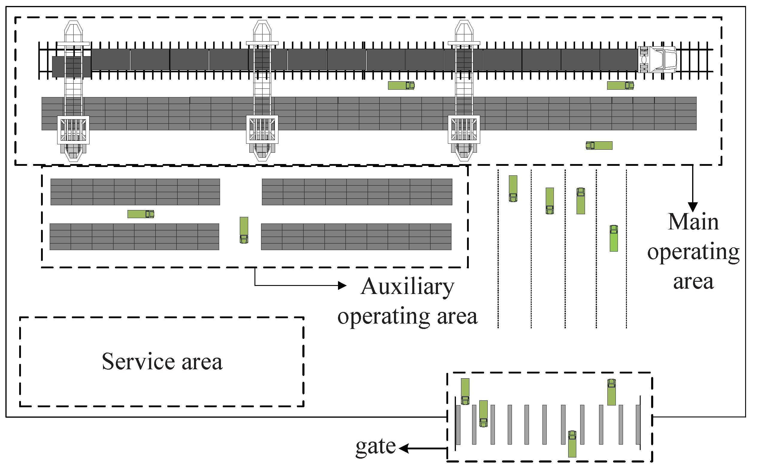
With the implementation of the “One Belt and Road” strategy and the increasing awareness of global environmental protection, railway container transportation has gradually become increasingly significant in comprehensive transportation system due to its integration advantages of container transportation and railway transportation, including safety, environmental protection, energy-saving, convenience, wide-coverage, and low freight rates. RCT is a vital support platform for railway container transportation. In the Eleventh Five-Year period, the Ministry of Transport of the People’s Republic of China and the Ministry of Railways of the People’s Republic of China jointly formulated “the mid-long term planning for China’s railway network”. The program proposed that eighteen large RCTs would be constructed in coastal and inland areas of China, including Dalian, Qingdao, and Chongqing. Now, twelve have been built and put into use. A transportation network of railway containers covering the whole country has been initially formed in China. The layout of the RCT is shown in Figure 1, e.g. Dalian Railway Container Terminal (DRCT), including four major sections, namely the main operation area, auxiliary operation area, service area, and gate. The main operation area of the RCT is responsible for storing, handling, collecting, and distributing containers. Owing to the high cost of handling resources, the RCT has difficulty purchasing additional equipment to improve operational performance. Therefore, the reasonable scheduling of its internal handling resources in the main operation area affects the service level, handling quality, and operation ability of the RCT.

In the main operating area, currently, most RCTs are equipped with huge GC as major handling equipment to improve the handling efficiency and accelerated the container turnover [1], such as DRCT, Chengdu Railway Container Central Terminal, Shanghai Container Central Station, etc. A few RCTs choose reach stackers (RSs) as their main equipment, such as Kunming Railway Container Terminal. There are significant differences in the operating equipment, handling plans, operating modes, storage methods, and container storage efficiency of these two RCTs. Some large-scale RCTs and sea–rail intermodal container terminals mostly use GCs as the main type of equipment for handling operations. Based on the above actual situation, this paper mainly focuses on the research of resource allocation and scheduling optimization for the RCT with GC as the main equipment.

The dual-GC spans the rail tracks, truck lanes, and storage yard, as shown in Figure 2. Most previous studies regarded GCs as the only handling resources in the main operating area [2,3,4,5,6,7,8]. However, GC has some obvious disadvantages of poor maneuverability, slower efficiency, higher energy consumption, and expensive handling costs, and the ITs in RCT have higher flexibility, faster travel speed, lower energy consumption, and lower transportation costs. Therefore, to avoid mutual interference between dual-GC, improve energy-saving, and reduce long-distance movement of each GC, we propose a new handling plan, that is “GCs-ITs”. Thus, when handling containers, the long-distance, full-loaded movement of GCs are replaced by ITs. At the same time, we develop a new yard partition strategy that divides handling areas for each crane to balance the workload of dual-GC, and the crane area may be crossing.

The crane is the critical bottleneck resource that affects operating performance whether in the port [9] or the RCT. Boysen et al. [10] reviewed the crane scheduling with interference in the seaport terminal, RCT, and warehousing. Kizilay and Elliyi [11] provided a comprehensive literature review about port handling operations, including quay crane (QC) operation, yard crane (YC) operation, and integrated operation.

Because of the early development of ports [12,13] and the increasing importance of intermodal transportation [14], the research on handling resource scheduling of the port is relatively mature. Zheng et al. [15] presented the scheduling problem of two YCs considering the real-time interference and the reshuffling operation. He et al. [16] addressed the YC scheduling problem considering the uncertainty of arrival time for task groups. Kaveshgar and Huynh [17] and Zhen et al. [18] introduced minimum temporal distance from Bierwirth and Meisel [19] to avoid the interference between two adjacent YCs. Bian et al. [20] proposed a loading scheduling problem of two YCs considering workload balance, parking time, and travel distance. Chen et al. [21] addressed the coordinated scheduling of QCs, ITs, and YCs to minimize the makespan of the ship. Yu and Yang [22] discussed the YC scheduling problem of hybrid storage container terminal considering the waiting time of external truck and ITs.

Comparing to the port, there are fewer studies on handling resource at RCT. Guo et al. [2,3] addressed the GC scheduling of RCT and rail-road container terminal considering crane interference and dwelling position of the train. Chang et al. [4,5] developed the coordinated scheduling problem of GCs, ITs, and YCs of RCT under the mixed handling mode. Besides, they further discussed the problem of storage space allocation. Zeng et al. [6] considered the operation sequence, non-crossing requirement, safety distance, and storage mode to address the problem of GC scheduling and slot allocation. Wang et al. [7] presented the GCs scheduling model to reduce idle time, and ant colony algorithm was developed to obtain solutions. Although the handling scheduling problem between the port and the RCT is similar, there are still great differences in the aspect of operation flow, yard layout, and handling resource types. Therefore, it is difficult for RCT to directly apply the related research results of the port.

As environmental protection awareness has increased, there is extensive literature on the reduction of energy consumption at the terminal. To reduce terminal congestion and carbon footprint, Facchini et al. [23,24] proposed a model-based Decision Support System (DSS) to seek the best strategy of inter-/intra-terminal flows of the containers among multiple terminals. He et al. [25] comprehensively considered the operational efficiency and energy consumption of the port to address coordinated scheduling of QCs, ITs, and YCs. Boysen et al. [26] discussed the train loading problem of GCs between road train and freight train to trade off the workload of GCs and energy consumption of road train. Tschoeke and Boysen [27] made a further discussion on container assignment and handling sequence to minimize the makespan of transshipment in RCT. Yang et al. [28] solved the integrated optimization of multiple equipment scheduling and storage space allocation with the bi-objective to minimize the operation time and energy consumption. Yue et al. [29] proposed the integrating scheduling of a dual-trolley QC and automatic guided vehicles (AGVs) to reduce energy consumption.

Studying the scheduling problem of multiple cranes, some papers design certain principles for dividing crane area to simplify the task assignment [7,8,30,31,32,33,34,35,36,37,38,39]. Boysen et al. [30,31,32] firstly developed the disjunctive crane area to avoid interferences among GCs in the rail-rail transshipment yard, rail-road transshipment yard, and quayside. However, the crane’s workload was determined by the full-loaded move, and the empty-loaded move was ignored. Wang and Zhu [7,8] presented the scheduling of GCs in RCT and rail-truck intermodal terminal based on the equal crane area to avoid interference. Fan et al. [33,34] presented the regional workload balance method to make a scheduling plan according to the number of YCs. Tang and Guo [35] divided the operation area of each GC according to the properties of containers.

Interrelation between handling resources scheduling and yard partition is complicated and challenging. Based on static disjunctive crane areas given in previous studies [30,31,32], Fedtke and Boysen [36,37] proposed optimization of the multiple GCs and shuttle car scheduling supported by the sorting system in rail-rail terminal. Wang et al. [38,39] developed a bi-layer optimization model to determine dynamic disjunctive crane area and schedule handling equipment included ITs and GCs, and a hybrid algorithm was designed to solve the model.

Recent studies mainly concentrate on the independent scheduling of GC and rarely consider the coordination between GCs and ITs at RCT. Existing literature on determining crane area is mostly the static, disjunctive, and equal principle. Most studies measure the performance of GC based on the task number, which is difficult to accurately reflect the management loss of equipment. Besides, several papers discuss the scheduling problem of handling equipment under the static crane area, ignoring the adverse effect of handling mode, scheduling plan, and container location on the decision of the crane area. In this paper, we solve the integrated allocation and scheduling problem of handling resources in the RCT based on the crossing crane area. The contributions are five aspects as follows:

• We determine the crossing crane area of dual-GC considering handling mode, scheduling plan, and container position instead of fixed, static, and disjunctive crane area, which increases the flexibility of GCs while avoiding interference.
• We balance the workload of dual-GC considering the full-loaded and empty-loaded distance, which can better reflect the operational performance.
• We discuss coordinated scheduling of GCs and ITs considering no-cross constraint and crossing area based on the “GCs-ITs” handling scheme. The scheme takes advantage of IT with higher flexibility, lower energy consumption, and lower operating costs to make up for the shortcomings of GC with lower mobility, higher energy consumption, and higher operating costs.
• We design TLHHA incorporating HR, ECEGA, GR, and SA to solve the multi-level, multi-stage, and two-way correlation optimization problem.
• We seek the best allocation and scheduling plan for the handling equipment of RCT. We develop an optimization model with multi-objectives, including maximizing the balance rate of dual-GC, minimizing the makespan, minimizing the handling cost, and minimizing energy consumption. The four objectives represent the four perspectives of performance, efficiency, effectiveness, and energy-saving. Our study provides theoretical support for the actual operation and management of the RCT.

The remainder of this paper is structured as follows. We describe the problem and develop a MIP model considering multi-objective in Section 2. In Section 3, we propose a TLHHA integrating HR, SA, ECEGA, and GR to solve the problem. Section 4 provides computational experiments to verify the correctness and validity of the proposed model and algorithm. In Section 5, we conclude this paper and propose future works.

2. Problem Description and Mathematical Model

2.1. Problem Description

When the train arrives at the RCT for handling operations, there are two handling modes under the “GCs-ITs” scheme, as depicted in Figure 3. Taking the outbound containers as an example, the GC loads the containers from the start position at the storage yard to the target position at the railcar. One is the direct move if both positions are located in the same crane area. The other is the split move if both positions lie in different crane areas. For that, one GC first picks up the container from the yard to the IT, then the IT transports it to the railcar, and finally it is picked up to the target position by another GC. The latter mode includes two sub-operations, namely unloading split move and loading split move. Whenever the target position is located far away from the start position, a reasonable combination of direct move and split move can effectively reduce the handling cost and improve the level of operational management of the RCT. However, it should be noted that the split move will cause twice the picking up and dropping process respectively of crane’s hoist.

Along the track, the positive direction is defined as the front to the rear of the train. The bay and row of storage, railcar, and GC are numbered as described in Figure 3. For ease of description, we introduce the unit of the crane area as slot [30,31,32]. The length of a slot is equal to the length of the unit bay or the railcar. The number of slots S is the maximum value between bay number B and railcar number A, that is $S=max(A,B)$. The driving carriageway in Figure 3 are dual and unidirectional to ensure operational safety and avoid collisions. ITs cannot turn round in the lane.

The decision problem is to optimize the allocation and scheduling of handling resources in the main operation area of the RCT. To more clearly understand the complicated and integrated problem, we subdivide it into four sub-problems. For outbound containers example, we study the integration of the four sub-problems considering the interaction between them.

• Yard partition problem (Q1): The working area of the track is divided for each GC. In independent crane areas, adjacent GCs work independently without interfering with each other. However, in the crossing areas, the non-cross constraints should be considered in real-time.
• Crane assignment (Q2): For containers that need to be operated, this sub-problem decides the handling mode according to the crane area, namely direct move or split move.
• Crane scheduling (Q3): The handling sequence of each GC is to be determined.
• IT scheduling (Q4): The IT participates in the handling operation only when the container adopts the split move. We assign the task and determine the transportation sequence for each IT.

2.2. Mathematical Formulation

2.2.1. Assumptions

The following are several assumptions for the mathematical formulation:

• All containers waiting for loading to the train are 40-feet equivalent unit (FEU).
• The start slot at the yard and target slot at the railcar of containers are assumed to be known in advance.
• Each container needed to be handled is regarded as a task.
• Each GC and IT has a virtual start and end task denoted as 0, and both virtual tasks are located at the initial position known in advance.

2.2.2. Notations and Variables

(1) Sets and parameters

I: the set of tasks, $i,j\in I$

G: the set of GCs, $g,g^{\prime }\in G=\{1,2\}$

S: the set of slots, $s,s^{\prime }\in S$

K: the set of ITs, $k,k^{\prime }\in K$

$P_i^1$: the start slot of task i

$P_i^2$: the target slot of task i

$r_i$: the row of task i at the yard

B: the number of bays at the yard

R: the number of rows at the yard

d: the distance between yard and track (unit:m)

$d_1$: the length of unit bay (unit:m)

$d_2$: the length of unit row (unit:m)

$\Gamma$: the pickup or drop time of GC (unit:s)

$v_1$: the average cart speed of GC (unit:m/s)

$v_2$: the average trolley speed of GC (unit:m/s)

$v_3$: the average speed of full-loaded IT (unit:m/s)

$v_4$: the average speed of empty-loaded IT (unit:m/s)

$c_1$: the unit moving cost of full-loaded GC (unit:yuan/m)

$c_2$: the unit moving cost of empty-loaded GC (unit:yuan/m)

$c_3$: the unit transportation cost of IT (unit:yuan/m)

$C_1$: the moving energy consumption of full-loaded GC unit distance (unit:kg/m)

$C_2$: the moving energy consumption of empty-loaded GC unit distance (unit:kg/m)

$C_3$: the waiting energy consumption for GC waited for IT unit second (unit:kg/s)

$C_4$: the moving energy consumption of full-loaded IT unit distance (unit:kg/m)

$C_5$: the moving energy consumption of empty-loaded IT unit distance (unit:kg/m)

$C_6$: the waiting energy consumption of IT waited for GC unit second (unit:kg/s)

M: a sufficiently positive integer

$\omega$: a weight coefficient transferring full-loaded distance to empty-loaded distance

(2) Decision variables

$\left[l_g,r_g\right]$: the crane area of GC g, where $l_g$ is left border and $r_g$ is right border

$X_{ig}$: if task i is operated by GC g using direct move, $X_{ig}=1$; otherwise, $X_{ig}=0$

$X_{ig}^{ul}$: if task i is unloaded by GC g using split move, $X_{ig}^{ul}=1$; otherwise, $X_{ig}^{ul}=0$

$X_{ig}^l$: if task i is loaded by GC g using split move, $X_{ig}^l=1$; otherwise, $X_{ig}^l=0$

$x_{ik}$: if task i is transported by IT k, $x_{ik}=1$; otherwise, $x_{ik}=0$

$y_{ij}$: if task i and j are operated by same GC, and i is immediate task for j, $y_{ij}=1$;

  otherwise, $y_{ij}=0$

$z_{ij}^k$: if task i and j are operated by same IT k, and i is immediate task for j, $z_{ij}^k=1$;

  otherwise, $z_{ij}^k=0$

${\psi }_{ij}$: if task i is executed before j, ${\psi }_{ij}=1$; otherwise, $a{\psi }_{ij}=0$

(3) Derived variables

$\pi$: if crane area of dual-GC is crossing, namely $l_1\le l_2\le r_1$, $\pi =1$; otherwise, $\pi =0$

$\left[l_g^1,r_g^1\right]$: the independent area of GC g, where $l_g^1$ is left border and $r_g^1$ is right border

$\left[l^2,r^2\right]$: the crossing area of dual-GC, where $l^2$ is left border and $r^2$ is right border

${\mu }_{ig}^1$: if the start slot of task i is within the independent area of GC g, namely,

  $l_g^1\le P_i^1\le r_g^1$, ${\mu }_{ig}^1=1$; otherwise, ${\mu }_{ig}^1=0$

${\chi }_{ig}^1$: if the target slot of task i is within the independent area of GC g, namely,

  $l_g^1\le P_i^2\le r_g^1$, ${\chi }_{ig}^1=1$; otherwise, ${\chi }_{ig}^1=0$

${\mu }_i^2$: if the start slot of task i is within the crossing area of dual-GC, namely,

  $l^2\le P_i^1\le r^2$, ${\mu }_i^2=1$; otherwise, ${\mu }_i^2=0$

${\chi }_i^2$: if the target slot of task i is within the crossing area of dual-GC, namely,

  $l^2\le P_i^2\le r^2$, ${\chi }_i^2=1$; otherwise, ${\chi }_i^2=0$

$I_g^d$: the task set of direct move operated by GC g

$I_g^{ul}$: the task set of unloading split move operated by GC g

$I_g^l$: the task set of loading split move operated by GC g

$I_g$: the task set handled by GC g, $I_g=I_g^d\vee I_g^{ul}\vee I_g^l$

$D_{gi}^1$: the cart moving distance of full-loaded GC g

$D_{gi}^2$: the trolly moving distance of full-loaded GC g

$E_{ij}^g$: the cart moving distance of empty-loaded GC g

$e_{ij}^g$: the trolley moving distance of empty-loaded GC g

$D_g$: the total distance of GC g after completing all task belong to it

$O_{gi}$: the beginning time of task i operated by GC g

$F_{gi}$: the finish time of task i operated by GC g

$W_i^{gk}$: the waiting time of GC g waited for IT k when operating task i

$o_{ki}$: the beginning time of task i operated by IT k

$f_{ki}$: the finish time of task i operated by IT k

$w_i^{kg}$: the waiting time of IT k waited for GC g when operating task i

${\tau }_{ki}$: the full-loaded moving time of IT k

${\xi }_{ij}^k$: the empty-loaded moving time of IT k

${\sigma }_{ki}^1$: the time when the IT k arrives at the start slot of task i

${\sigma }_{ki}^2$: the time when the IT k arrives at the target slot of task i

2.2.3. Objectives

We formulate the optimization model with multi-objective as expressed in Equations (1)–(4). Objective 1 is to maximize the balance rate of dual-GC expressed by the ratio of the smallest moving distance to the largest. Objective 2 is to minimize the makespan of the handling operation. Objective 3 seeks to minimize the handling cost, including the full-loaded and empty-loaded moving cost of dual-GC and the transportation cost of ITs. Objective 4 is to minimize the energy consumption of ITs and GCs.

$$Objective1:max{Z}_1=\left[min\left(D_g\right)/max\left(D_g\right)\right],\forall g\in G$$

(1)

$$Objective2:min{Z}_2=\underset{g\in G,i\in I}{max}\left(F_{gi}\right)$$

(2)

$$\begin{array}{cc}\hfill Objective3:min{Z}_3=& c_1\sum _{g\in G}\sum _{i\in I}{D}_{gi}^1+c_2\sum _{g\in G}\sum _{i\in I\vee \{0\}}\sum _{j\in I\vee \{0\}}{E}_{ij}^g+\hfill \\ \hfill & c_3\left(\sum _{k\in K}\sum _{i\in I}{\tau }_{ki}·v_3+\sum _{k\in K}\sum _{i\in I\vee \{0\}}\sum _{j\in I\vee \{0\}}{\xi }_{ij}^g·v_4\right)\hfill \end{array}$$

(3)

$$\begin{array}{cc}\hfill Objective4:min{Z}_4=& \left(C_1\sum _{g\in G}\sum _{i\in I}{D}_{gi}^1+C_2\sum _{g\in G}\sum _{i\in I\vee \{0\}}\sum _{j\in I\vee \{0\}}{E}_{ij}^g\right)\hfill \\ \hfill & +\left(C_4\sum _{k\in K}\sum _{i\in I}{\tau }_{ki}·v_3+C_5\sum _{k\in K}\sum _{i\in I\vee \{0\}}\sum _{j\in I\vee \{0\}}{\xi }_{ij}^g·v_4\right)\hfill \\ \hfill & +\left(+C_3\sum _{g\in G}\sum _{k\in K}\sum _{i\in I}{W}_i^{gk}+C_6\sum _{k\in K}\sum _{g\in G}\sum _{i\in I}{w}_i^{kg}\right)\hfill \end{array}$$

(4)

2.2.4. Constraints

In Section 2.2.4, we express the corresponding constraints on the integrated allocation and scheduling of handling resources in the RCT. Equations (5)–(9) are constraints on the yard partition problem. Equations (10)–(18) represent constraints on crane assignment. Equations (19)–(22) are constraints on crane scheduling. Equations (23)–(27) are constraints on IT assignment and scheduling. Equations (28)–(38) are constraints on the cohesion of handling equipment. Equations (39)–(41) are on non-interference of multiple GCs. Equations (42)–(44) are the constraints on the values of variables.

$$r_{g-1}+1\le r_g\le S-G+g,\forall g\in G$$

(5)

$$l_1\le l_2\le r_1+1$$

(6)

$$l^2=\pi ·l_2,r^2=\pi ·r_2$$

(7)

$$l_1^1=1,l_2^1=r_1+1$$

(8)

$$r_1^1=l_2-1,r_2^1=S$$

(9)

Equations (5) and (6) indicate the right border and the left border of GC g. Equation (7) defines the left and right board of the crossing crane area of dual-GC. Equations (8) and (9) define the left and right board of the independent crane area of each GC.

$${\mu }_{ig}^1{\chi }_{ig}^1\le X_{ig},\forall i\in I,g\in G$$

(10)

$${\mu }_{ig}^1{\chi }_{i{g}^{\prime }}^1\le X_{ig}^{ul}{X}_{i{g}^{\prime }}^l,\forall i\in I,g,g^{\prime }\in G,g\ne g^{\prime }$$

(11)

$${\mu }_{ig}^1{\chi }_i^2\le \left(X_{g^{\prime }}^l{X}_g^{ul}\right)+X_{ig},\forall i\in I,g,g^{\prime }\in G,g\ne g^{\prime }$$

(12)

$${\mu }_i^2{\chi }_{ig}^1\le \left(X_g^l{X}_{g^{\prime }}^{ul}\right)+X_{ig},\forall i\in I,g,g^{\prime }\in G,g\ne g^{\prime }$$

(13)

$${\mu }_i^2{\chi }_i^2\le X_{i1}^{ul}{X}_{i2}^l+X_{i1}+X_{i2}+X_{i1}^l{X}_{i2}^{ul},\forall i\in I$$

(14)

$$I_g^d=\left\{i\mid X_{gi}=1,i\in I\right\},\forall g\in G$$

(15)

$$I_g^{ul}=\left\{i\mid X_{gi}^{ul}=1,i\in I\right\},\forall g\in G$$

(16)

$$I_g^l=\left\{i\mid X_{gi}^l=1,i\in I\right\},\forall g\in G$$

(17)

$$1\le \sum _{g\in G}\left(X_{ig}^{ul}+X_{ig}^l+X_g\right)\le 2,\forall i\in I$$

(18)

Equations (10)–(14) assign the handling mode of all tasks to dual-GC according to the crane area. For task i, direct move must be adopted if the start and target slot are within the independent area of GC g, whereas split move must be used if both slots are located in the different independent areas of dual-GC as represented in Equations (10) and (11). Equations (12)–(14) indicate either direct move or split move if one slot lies in the independent area and the other slot lies in the crossing area, or both slots are within the crossing area. Equations (15)–(17) define the task set operated by each GC. Equation (18) means any task should be conducted by at least one GC and at most two GCs.

$$\sum _{i\in I_g\vee \{0\}}{y}_{ij}=1,\forall g\in G,j\in I_g\vee \{0\},i\ne j$$

(19)

$$\sum _{j\in I_g\vee \{0\}}{y}_{ij}=1,\forall g\in G,j\in I_g\vee \{0\},i\ne j$$

(20)

$$y_{ij}\le 0.5\left[\left(X_{ig}+X_{ig}^{ul}+X_{ig}^l\right)+\left(X_{jg}+X_{jg}^{ul}+X_{jg}^l\right)\right],\forall i,j\in I_g\vee \{0\},g\in G$$

(21)

$$\sum _{i\in I^{\prime }}\sum _{j\in I^{\prime }}{y}_{ij}\le \left|I^{\prime }\right|-1,\forall I^{\prime }\subseteq I_g,\left|I^{\prime }\right|\ge 2$$

(22)

Equations (19) and (20) define the job sequence of GCs, indicating each task for GC has only one task as an immediate predecessor and one task as an immediate follower. Equation (21) defines the relationship of decision variables between crane assignment and crane scheduling. Equation (22) avoids the sub-circuit of each GC operation.

$$\sum _{k\in K}{x}_{ik}=1,\forall i\in {\vee }_{g\in G}{I}_g^{ul}$$

(23)

$$\sum _{i\in {\vee }_{g\in G}{I}_g^{ul}\vee \{0\}}{z}_{ij}^k=1,\forall k\in K,j\in {\vee }_{g\in G}{I}_g^{ul}\vee \{0\},i\ne j$$

(24)

$$\sum _{j\in {\vee }_{g\in G}{I}_g^{ul}\vee \{0\}}{z}_{ij}^k=1,\forall k\in K,i\in {\vee }_{g\in G}{I}_g^{ul}\vee \{0\},i\ne j$$

(25)

$$z_{ij}^k\le 0.5\left(x_{ik}+x_{jk}\right),\forall i,j\in {\vee }_{g\in G}{I}_g^{ul}\vee \{0\},i\ne j$$

(26)

$$\sum _{i\in I^{\prime }}\sum _{j\in I^{\prime }}{z}_{ij}^k\le \left|I^{\prime }\right|-1,\forall k\in K,I^{\prime }\subseteq {\vee }_{g\in G}{I}_g^{ul}, \left|I^{\prime }\right|\ge 2$$

(27)

Equation (23) ensures that each task of the split move is operated by an IT. For each IT, Equations (24) and (25) indicate each task has only one task as an immediate predecessor and one task as an immediate follower. Equation (26) defines the relationship between IT assignment and IT scheduling. Equation (27) avoids the sub-circuit of each IT operation.

$$F_{gi}\ge O_{gi}+2\Gamma +max\left(D_{gi}^1/v_1,D_{gi}^2/v_2\right),\forall i\in I_g,g\in G$$

(28)

$$\begin{array}{cc}\hfill O_{gi}-& \left[F_{gi}+max\left(E_{ij}^g/v_1,e_{ij}^g/v_2\right)+W_i^{gk}\right]+\left(1-y_{ij}\right)M\ge 0,\hfill \\ \hfill & \forall i,j\in I_g\vee \{0\},i\ne j,g\in G,k\in K\hfill \end{array}$$

(29)

$$O_{gi}+\left(3-x_{ik}-X_{i{g}^{\prime }}^{ul}-X_{ig}^l\right)M\ge F_{g^{\prime }i}+{\tau }_{ki},\forall i\in I_g^l\wedge I_{g^{\prime }}^{ul},g,g^{\prime }\in G,g\ne g^{\prime },k\in K$$

(30)

$$\left(O_{gi}-{\sigma }_{ki}^1\right)+\left(1-x_{ik}\right)M\ge 0,\forall i\in I_g^{ul},g\in G,k\in K$$

(31)

$$\left(O_{gi}-{\sigma }_{ki}^2\right)+\left(1-x_{ik}\right)M\ge 0,\forall i\in I_g^l,g\in G,k\in K$$

(32)

$$o_{ki}-F_{gi}+\left(1-x_{ik}\right)M\ge 0,\forall i\in I_g^{ul},g\in G,k\in K$$

(33)

$$f_{ki}+\left(1-x_{ik}\right)M\ge O_{gi}+\Gamma +0.5d/v_2,\forall i\in I_g^l,g\in G,k\in K$$

(34)

$${\sigma }_{kj}^1+\left(1-z_{ij}^k\right)M\ge f_{ki}+{\xi }_{ij}^k,\forall i,j\in I_g^{ul}\vee I_g^l\vee \{0\},g\in G,k\in K,i\ne j$$

(35)

$${\sigma }_{kj}^2+\left(1-x_{ik}\right)M\ge o_{ki}+{\tau }_{ki},\forall i,j\in I_g^{ul}\vee I_g^l\vee \{0\},g\in G,k\in K$$

(36)

$$f_{ki}+\left(1-x_{ik}\right)M\ge o_{ki}+{\tau }_{ki}+w_i^{kg},\forall i\in I_g^{ul}\vee I_g^l\vee \{0\},g\in G,k\in K$$

(37)

$$o_{ij}+\left(1-z_{ij}^k\right)M\ge f_{kj}+{\xi }_{ij}^k+w_j^{kg},\forall i\in I_g^{ul}\vee I_g^l\vee \{0\},j\in I_g^{ul},g\in G,k\in K,i\ne j$$

(38)

Equations (28) and (29) define the cohesion of single GC. Equation (28) expresses the relationship between the finish time and the start time of a task operated by a GC. Equation (29) indicates that the time constraint of two consecutive tasks for a GC. For split move, Equation (30) indicates the cohesion between two different GCs that the start time of the loading move must later than the finish time of the unloading move. Equations (31)–(34) define the cohesion of time between GCs and ITs. For split move, Equations (31) and (32) indicate the connection between the start time of the GC and the arrival time of the IT; Equation (33) is the cohesion between the start time of the IT and the finish time of the GC; and Equation (34) is the cohesion between the finish time of the IT and the start time of the GC. Equations (35)–(38) define the cohesion of single IT. Equations (35) and (36) express the arrival time of the IT at the yard or railcar. Equation (37) expresses the relationship between the finish time and the start time of a task operated by an IT. Equation (38) indicates the time constraint of two consecutive tasks for an IT.

$$F_{gi}-S_{g^{\prime }j}\le M\left(1-{\psi }_{ij}\right),\forall i\in I_g,j\in I_{g^{\prime }},g,g^{\prime }\in G,g\ne g^{\prime }$$

(39)

$$S_{g^{\prime }j}-F_{gi}\le M{\psi }_{ij},\forall i\in I_g,j\in I_{g^{\prime }},g,g^{\prime }\in G,g\ne g^{\prime }$$

(40)

$$\begin{array}{cc}\hfill & M({\psi }_{ij}+{\psi }_{ji})\ge \sum _{i^{\prime }\in I_g\vee \{0\}}{y}_{i^{\prime }i}^1+\sum _{i^{\prime }\in I_g\vee \{0\}}{y}_{i^{\prime }i}^2-1,\forall (i,j)\in \{(i,j)|{\mu }_i^2+{\chi }_i^2\ge 1,\hfill \\ \hfill & {\mu }_j^2+{\chi }_j^2\ge 1,(X_{i1}+X_{i1}^{ul})P_i^1+X_{i1}^l{P}_i^2\ge (X_{j2}+X_{j2}^{ul})P_j^1+X_{j2}^l{P}_j^2,i\in I_1,j\in I_2\}\hfill \end{array}$$

(41)

Equations (39) and (40) define the binary variable ${\psi }_{ij}$. Equation (41) ensures adjacent GCs do not cross if ${\psi }_{ij}+{\psi }_{ji}=0$.

$$(l_g,r_g,l_g^1,r_g^1,l^2,r^2)\in {\mathbb{Z}}^{+},(I_g^d,I_g^{ul},I_g^l,I_g)\in \mathbb{N},\forall g\in G$$

(42)

$$(X_{ig},X_{ig}^{ul},X_{ig}^l,x_{ik},y_{ij},z_{ij}^k,{\psi }_{ij},\pi ,{\mu }_{ig}^1,{\chi }_{ig}^1,{\mu }_i^2,{\chi }_i^2)\in \{0,1\},\forall g\in G,i,j\in I\vee \{0\},k\in K$$

(43)

$$(D_{gi}^1,D_{gi}^2,E_{ij}^g,e_{ij}^g,D_g,O_{gi},F_{gi},W_i^{gk},o_{ki},f_{ki},w_{kg}^i,{\tau }_{ki},{\xi }_{ij}^k,{\sigma }_{ki}^1,{\sigma }_{ki}^2)\ge 0,\forall g\in G,i,j\in I\vee 0,k\in K$$

(44)

Equations (42)–(44) define variables.

2.2.5. Calculation of Movement Distance and Time of Handling Resources

1. Calculation of full-loaded movement distance of GC

In the “GCs-ITs” handling scheme, the cart movement distance of full-loaded GC only occurs when the task is handled by direct mode, as represented in Equation (45).

$$D_{gi}^1=X_{ig}|P_i^1-P_i^2|d_1,\forall i\in I,g\in G$$

(45)

The trolley moving distance of full-load GC is related to handling mode as shown in Equation (46).

$$D_{gi}^2=X_{gi}\left(r_i{d}_2+d\right)+X_{gi}^{ul}\left(r_i{d}_2+0.5d\right)+0.5X_{gi}^{l}d,\forall g\in G,i\in I$$

(46)

We measure the performance of the GC by the total moving distance $D_g$ in objective 1. We adopt the parameter $\omega$ to balance the full-loaded and empty-loaded moving distance by converting the former to the latter, as shown in Equation (47).

$$D_g=\omega \sum _{i\in I}{D}_{gi}^1+\sum _{i\in I_g\vee \{0\}j\in I_g\vee \{0\}}{E}_{ij}^g,\forall g\in G$$

(47)

2. Calculation of empty-loaded movement distance of GC

The empty-loaded movement of GC is represented in Equations (48) and (49) when handling two consecutive tasks, including four situations: yard to yard, railcar to railcar, yard to railcar, and railcar to yard.

$$\begin{array}{cc}\hfill & E_{ij}^g=y_{ij}{d}_1\{[X_{ig}^l(X_{jg}+X_{jg}^{ul})+X_{ig}(X_{jg}+X_{jg}^{ul})]|P_i^2-P_j^1|+X_{ig}^{ul}{X}_{jg}^l|P_i^1-P_j^2|+\hfill \\ \hfill & [(X_{ig}^l+X_{ig})X_{jg}^l]|P_i^2-P_j^2|+[X_{ig}^{ul}(X_{jg}^{ul}+X_{jg})]|P_i^1-P_j^1|\},\forall i,j\in I_g\vee \{0\},g\in G\hfill \end{array}$$

(48)

$$\begin{array}{c}{e}_{ij}^g=y_{ij}\{[(X_{ig}+X_{ig}^l)(X_{jg}+X_{jg}^{ul})](d+r_j{d}_2)+X_{ig}^{ul}(X_{jg}+X_{jg}^{ul})|r_i-r_j|d_2+\\ X_{ig}^{ul}{X}_{jg}^l(d+r_i{d}_2)\}\forall i,j\in I_g\vee \{0\},g\in G\end{array}$$

(49)

3. Calculation of traveling time of IT

The IT lanes are unidirectional, so the traveling time of IT is related to the start and target slot of the task, as in Equations (50) and (51).

$${\tau }_{ki}=\left\{\begin{array}{c}{x}_{ik}\left|P_i^1-P_i^2\right|d_1/v_3,P_i^1\ge P_i^2\hfill \\ x_{ik}\left[\left(\left|P_i^1-P_i^2+2B+1\right|\right)d_1+2R{d}_2\right]/v_3,P_i^1<P_i^2,\hfill \end{array}\right.\forall i\in {\vee }_{g\in G}{I}_g^{ul},k\in K$$

(50)

$${\xi }_{ij}^k=\left\{\begin{array}{c}\left.z_{ij}^k\left|P_i^2+2B-P_j^1+1\right|l+2R{d}_2\right)/v_4,P_i^2<P_j^1,\hfill \\ z_{ij}^k\left|P_i^2-P_j^1\right|d_1/v_4,P_i^2\ge P_j^1\hfill \end{array}\right.\forall (i,j)\in {\vee }_{g\in G}{I}_g^{ul},k\in K$$

(51)

4. The waiting time of handling equipment

For split move, waiting time refers to the failing cohesion between the GC and IT. The waiting time of the GC waited for the IT and the IT waited for GC can be presented as Equations (52) and (53).

$$W_j^{gk}=\left\{\begin{array}{c}max〈\{{\sigma }_{ij}^1-[F_{gi}+max(E_{ij}^g/v_1,e_{ij}^2/v_2)]\},0〉,\forall i,j\in I_g^{ul}\vee \{0\}\hfill \\ max〈\{{\sigma }_{ij}^2-[F_{gi}+max(E_{ij}^g/v_1,e_{ij}^g/v_2)]\},0〉,\forall i,j\in I_g^l\vee \{0\}\hfill \end{array}\right.\forall g\in G,k\in K$$

(52)

$$w_i^{kg}=\left\{\begin{array}{c}max(S_{gi}-{\sigma }_{kj}^1,0),\forall i\in I_g^{ul}\hfill \\ max(F_{gi}-{\sigma }_{ij}^2,0)+0.5d/v_2+\Gamma ,\forall i\in I_g^l\hfill \end{array}\right.\forall g\in G,k\in K$$

(53)

3. Solution Algorithm

3.1. Overall Framework

The integrated scheduling problem of RCT resources is a multi-level, multi-stage, and two-way correlation optimization problem, including four sub-problems whose relationship is shown in Figure 4. Q1 is the basis for Q2 to make decision, and the result of Q2 influences Q3. There is a two-way relationship between Q3 and Q4. Besides, Q3 has a counter-effect to Q1, so they are two-level planning problems, while Q2, Q3, and Q4 are three-stage optimization problems. Q1 and Q2 have been proved to be NP-hard problems [18,30,31,32], and the scientific basis of Q3 and Q4 are both m-TSP classified as NP-hard problems. Therefore, the integrated scheduling problem is a complicated NP-hard problem. It is difficult to obtain the optimal solution in a reasonable time by using an accurate algorithm or commercial solvers. We propose TLHHA considering the characteristics of the model and problem to obtain the solution.

The overall framework of TLHHA is shown in Figure 4. The first layer adopts HR to solve Q1 and the satisfying balance rate is set as the termination condition. The second layer uses SA to decide Q2, and the termination condition is the end temperature. The three-layer fusion of ECEGA and GR is used to solve the coordinated optimization Q3 and Q4, and the termination condition is the maximum iterations.

Specifically, firstly, the crossing crane area is initialized based on trisection as represented $A_1,A_2,A_3$. The independent crane area of two GCs are $A_1+A_2$ and $A_2+A3$ separately, and the crossing area is $A_2$. Based on the assignment of the crane area, the task assignment is initialized. Then, perform the down-top iteration. In particular, the scheduling sequences of dual-GC are obtained by ECEGA, and the IT scheduling plan is solved by GR. Return the scheduling result of dual-GC to the second layer to obtain the best task allocation. Finally, after returning the results of the following two layers to the first layer, HR is used to adjust the crane area. After adjusting, perform top-down iteration. The flowchart of this procedure is shown in Figure 5, where $gen$ is the the current generation; $max\_gen$ represents the maximum iteration, L expresses the length of the Metropolis chain, l is the current chain, $T_0$ and $Tend$ are the initial and termination temperature apart, T is the current temperature, and q is the cooling rate. The objective Z is defined in Equation (55).

3.2. Algorithm Strategy

3.2.1. Encoding and Decoding Strategy for Task Allocation of Dual-GC

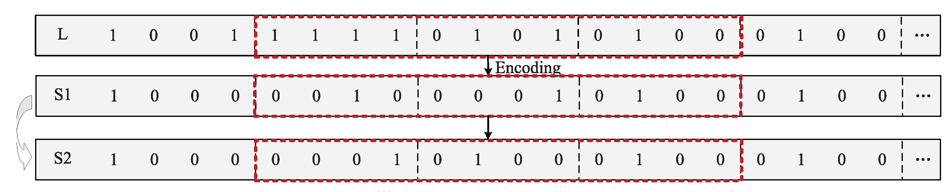
For each task, there are four possible operating modes: the direct move by GC 1, the direct move by GC 2, unloaded by GC 1 and loaded by GC 2 of the split move, and unloaded by GC 2 and loaded by GC 1 of the split move. Based on the crane area, the possible operating modes L of each task can be determined, as shown in Figure 6. For each task, select an operating mode to compose S1, that is, in every four columns of L, there is only one sequence of 1. Furthermore, there is 0 in L, which must be 0 in S1.

In ECEGA, the problem of dual-GC scheduling is represented as a three-dimensional chromosome by the sequence encoding method, as shown in Figure 7. Line 1 represents the operation sequence of dual-GC. Line 2 is the GC operating the corresponding task. Line 3 expresses the operating mode of dual-GC, where 0 is direct move, 1 is loading split move, and −1 is unloading split move.

3.2.2. Strategy of Repair and Penalty for Unfeasible Chromosome

There may be unfeasible solutions for randomly generated initial populations and offspring of dual-GC scheduling. The unfeasible solutions chiefly include the following three scenarios. For the first two scenarios, we design the gene repair procedure to repair unfeasible chromosomes, and for the third scenario, the penalty strategy is used to dispose of unfeasible chromosomes.

Scenario 1: Operating modes of the first task performed by both GCs are 1, which would cause them to wait for each other, and neither can start the operation. The principle of gene repair is to only change the operating sequence of conflicting tasks. Find out if there is a direct move in GC 1. If so, change the operation sequence between the task and the first loading task of the split move. If not, use the same method to find the GC 2, as shown in Figure 8.

Scenario 2: If one GC operates two tasks by loading and unloading of split move successively, corresponding to these two tasks operated in the opposite sequence by the split move for the other GC, so that two GCs would wait for each other and could not continue the operation. The principle of gene repair is to change the operating sequence of two conflicting tasks in GC 1, as shown in Figure 9.

Scenario 3: If dual-GC cannot meet the non-crossing constraint in equations (39)–(41) during operation shown in Figure 10, the unfeasible solution appears. For that, the fitness function is 0, so that the individual is eliminated in the genetic loop operation.

3.2.3. IT Allocation and Scheduling Strategy

IT is not a critical bottleneck resource for RCT. Considering Objectives 2–4 and using a minimum number of ITs, the GR is adopted to optimize Q4. According to the operation sequence of dual-GC, the first IT that arrives at the start slot of the current unloading task operated by the split move is selected to perform the horizontal transportation operation.

3.2.4. Genetic Operators of ECEGA

The affinity between the elite individual and the global optimal solution is greater than between other individuals and the latter. The elite individuals play an important role in evolution. Therefore, the traditional genetic algorithm (GA) using the elite strategy can quickly converge to the global optimal solution. Co-evolution genetic algorithm (CEGA) emphasizes the mutual influence and co-evolution of multiple populations, which can effectively avoid premature convergence and local optimization brought by GA. Therefore, to speed up the algorithm convergence, while ensuring the diversity of the population and avoiding the algorithm’s premature maturity, we propose ECEGA to solve Q3.

1. Parent selection strategy

The GA usually uses the roulette wheel selection operator. With the increase of evolutionary iteration, the fitness of the individual and the homogeneity of the population gradually increased. It is easy to cause the algorithm to mature prematurely and fall into the local optimum. To solve this problem, considering the global convergence and population diversity of the algorithm comprehensively, individuals with higher fitness values and larger chromosomal differences are selected to form two subpopulations. The calculation formula for the difference between individuals is as follows:

$$\left\{\begin{array}{c}c{h}_{il}=c{h}_{jl}\to \left(c{h}_{il},c{h}_{jl}\right)=0,c{h}_{il}\ne c{h}_{jl}\to \left(c{h}_{il},c{h}_{jl}\right)=1\hfill \\ {\delta }_{ij}=1/\ell {\displaystyle \sum _{l=1}^{\ell }}\left(c{h}_{il},c{h}_{jl}\right)\hfill \end{array}\right.$$

(54)

where i and j are individuals, l is the gene, ℓ is the length of gene, and $c{h}_{il}$ represents the value of individual i of gene l. The difference between the two chromosomes ${\delta }_{ij}$ is the mean value of the gene difference across the ℓ genes.

The selection strategy is as follows: supposing the population size is N and the tth population is $po{p}_t$, we find the elite individual $El(t)$. Divide the population into two subgroups. First, we select $N/4$ individuals to form one sub-group $po{p}_1(t)$ according to the roulette wheel selection operator. Then, we calculate the difference between each individual and $El(t)$. Using the idea of the roulette wheel selection operator by regarding ${\delta }_{ij}$ as a fitness function, select individuals to form the other subgroup $po{p}_2(t)$.

2. Order crossover operator and swap mutation operator

The encoding of dual-GC scheduling problem is more complicated. To reduce the complexity of the genetic operation and the infeasibility of solutions, the order crossover operator and swap mutation operator are adopted [16,25]. For the swap mutation operator, two mutation points should be randomly selected in the operation sequence of same GC.

3. Co-evolution strategy to generate new populations

We adopt co-evolution technology to generate new populations. First, for the subgroups $po{p}_1(t)$ and $po{p}_2(t)$ of each generation, cross and mutate them with elite individuals $El(t)$ to produce $N/2$ offspring separately. Then, for the subgroup $po{p}_1(t)$, cross and mutate them in pairs randomly to produce $N/4$ offspring. For $5N/4$ individuals, repair and dispose of the unfeasible solution. Calculate and sort the fitness of the individual in ascending order, select the first $N-1$ individuals and $El(t)$ to form a new generation of the population.

3.2.5. Fitness Function

According to prior experiments, the relationship between objectives 2 and 3 is $2Z_3\le Z_2\le 3Z_3$ and between objectives 2 and 4 is $15Z_4\le Z_2\le 20Z_4$. Therefore, for ECEGA, to keep the magnitude of each objective consistent, the fitness function shows as Equation (55) to find the optimal scheduling method for dual-GCs and ITs, where $\gamma$ is the weight of objective j.

$$\begin{array}{cc}\hfill & \mathrm{fintness}=1/Z\hfill \\ \hfill & \mathrm{st}.\left\{\begin{array}{c}Z={\gamma }_1{Z}_2+2{\gamma }_2{Z}_3+15{\gamma }_3{Z}_4\hfill \\ \left({\gamma }_j\ge 0,{\displaystyle \sum _{j=2}^4}{\gamma }_j=1,j=\{2,3,4\}\right)\hfill \end{array}\right.\hfill \end{array}$$

(55)

3.2.6. Neighborhood Search for SA

For neighborhood search for SA, the current solution $S_1$ is randomly disturbed to produce a new solution $S_2$. Two points are randomly generated, for example, $r_1=2$ and $r_2=4$, that is Tasks 2–4. At the same time, if the sequence of L is 0, the new solution $S_2$ is still 0. An operating move is randomly generated for selected tasks so that one code is 1 and the others are all 0. If there is only one operating move of the task in L, its code remains unchanged. In Figure 11, Task 4 has only one operating move; the randomly generated position of Tasks 2 and 3 are 4 and 2, respectively; and the new solution $S_2$ is produced.

3.2.7. Adjustment Strategy for Crane Area

HR is applied to adjust the crane area. Equation (56) calculates the number of slots $\Delta$ needed to be adjusted. Based on $\Delta$, there are three types of adjustment strategies as follows. The final selected strategy is to make Objective 1 greater than the satisfying balance rate, while Objectives 2–4 are minimizing.

Strategy 1: Increase the crane area $\Delta$ of GC whose moving distance is less than the average value.

Strategy 2: Decrease the crane area $\Delta$ of GC whose moving distance is greater than the average value.

Strategy 3: Take Strategies 1 and 2 at the same time.

$$\Delta =\frac{\left|D_1-\left(D_1+D_2\right)/2\right|}{\left(D_1+D_2\right)/S}$$

(56)

4. Computational Experiments

Some computation experiments were conducted to test the effectiveness of the proposed optimization model and TLHHA. Firstly, some initial settings were introduced. Secondly, some experiments were conducted with different division rules for crane areas to evaluate the performance of our solution. Besides, we compared the computational time and solution quality of four methods: HR-ECEGA-SA, HR-CEGA -SA (designed by Wang et al. [38]), HR-GA-SA, and CPLEX. Thirdly, sensitivity analyses were performed to demonstrate the varieties of each objective with varied stopping position of the train and number of ITs. All experiments were run on a PC with Intel(R) Core(TM) i7-7700 CPU @ 3.60 GHz processors and 8 GB RAM.

4.1. Experiments Design

The layout from DRCT is introduced as background and the schematic is shown in Figure 1. Actual data from DRCT were collected to conduct all experiments, as shown in

Table 1. Basic parameters of RCT.

Parameters	Quantity
Initial slot for GCs/ITs	slots (8,38)/slot 44
Balance parameter for distance/Weight of objectives 2–4	1.5/[0.4,0.4,0.2]
Length/width of unit bay/Distance between track and yard(m)	13/2.6/
Cart/Trolley speed(m/s)	1.33/1.42
Pick up/drop time(s)	60/60
Speed of full-loaded/empty-loaded IT(m/s)	5.5/8.3
Operational cost of full-loaded/empty-loaded GC(yuan/m)	0.5/0.4
Transportation cost of IT(yuan/km)	5.5
Moving energy consumption of full-loaded/empty-loaded GC(kg/m)	0.0337/0.0259
Waiting energy consumption for GC waited for IT/IT waited for GC(kg/s)	0.0138/0.0111
Moving energy consumption of full-loaded/empty-loaded IT(kg/m)	0.0107/0.0080

. The train has 45 railcars, whose capacity is 45 FEU containers. For a case, 30 FEU containers are waiting to be loaded from the yard to railcars, and their location information is shown in

Table 2. Location information for 30 FEU containers.

Numbers	Bays	Railcars	Rows	Numbers	Bays	Railcars	Rows	Numbers	Bays	Railcars	Rows
1	1	2	1	11	25	16	3	21	34	33	4
2	1	3	4	12	18	18	2	22	30	35	5
3	3	4	2	13	19	19	3	23	28	36	3
4	6	6	3	14	14	21	2	24	27	37	5
5	5	7	4	15	17	23	3	25	34	38	2
6	9	8	5	16	24	25	5	26	29	39	2
7	13	9	2	17	27	27	4	27	31	40	5
8	21	12	4	18	27	28	2	28	34	42	1
9	22	14	5	19	29	30	4	29	33	43	5
10	22	15	4	20	32	31	3	30	35	45	3

. The yard has 35 bays, 5 rows, and 4 layers, and each storage slot can store one FEU container. The track is equipped with dual-GC and three ITs. The first railcar is numbered 1. The stop position 5 means that the first bay is numbered 5. The population size of ECEGA is 200. The crossover probability and mutation probability are 0.9 and 0.05, respectively, and the maximum number of iterations is 500. The initial and termination temperature of SA are 1000 and 1 × 10${}^{-3}$, respectively. The cooling rate is 0.9, and the length of the Metropolis chain is 50. The balance rate of dual-GC is 90%.

4.2. Experiment Results

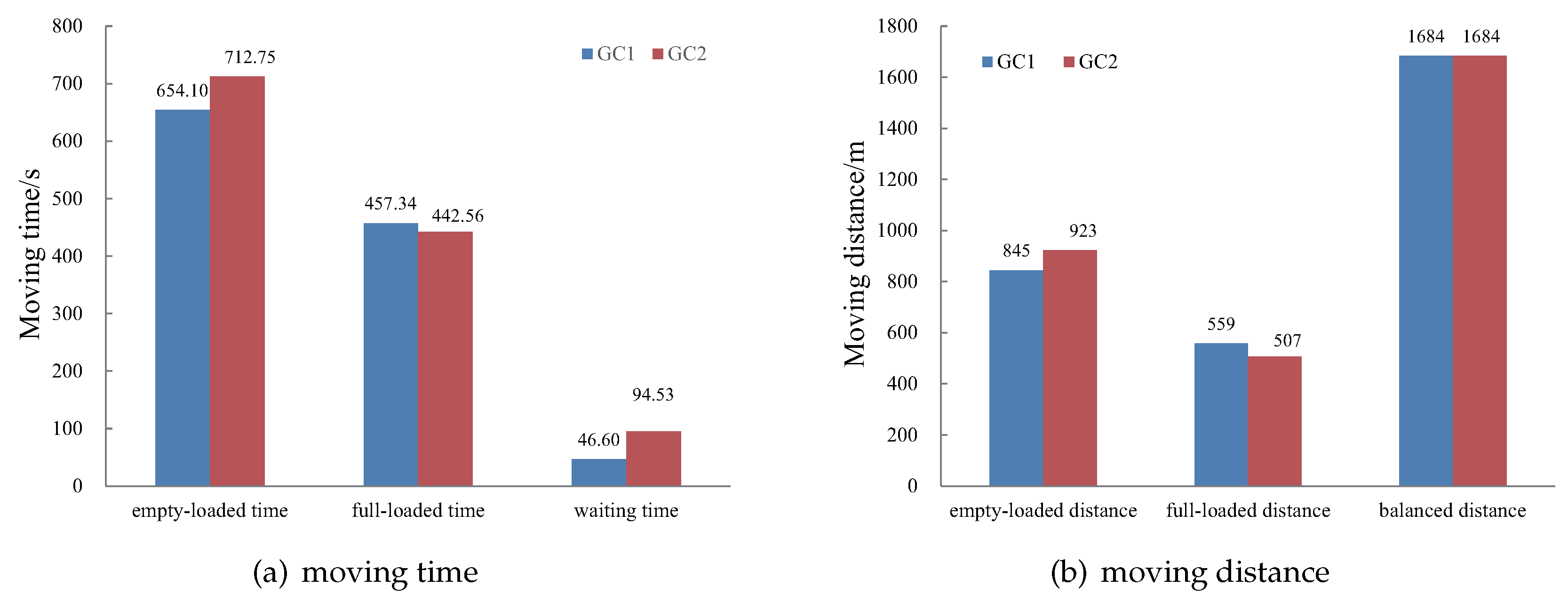
Calculating the test expressed in Table 2, the CPU time of TLHHA is 328.85 s. The best crane area of dual-GC is slot 1-slot 32 and slot 14-slot 45. Therefore, the independent crane areas of GC 1 and GC 2 are slot 1-slot 13 and slot 33-slot 45, respectively, and the crossing crane area is slot 14-slot 32. The balanced rate of dual-GC is 100%. The total moving distance of two GCs after balancing is 1683.5 m. The makespan, handling cost, and energy consumption are 3289.17 s, 1383.77 yuan, and 214.39 kg, respectively. The optimal scheduling scheme is shown in

Table 3. Scheduling scheme of dual-GC and three ITs.

Equipments	Number of Tasks	Scheduling Sequence
GC1	20	11(−1)→20(1)→23(−1)→24(−1)→17(0)→16(0)→15(0)→13(0)→7(0)→4(0)→
		3(0)→1(0)→2(0)→5(0)→14(0)→12(1)→10(1)→9(1)→8(1)→6(0)
GC2	18	19(0)→20(−1)→27(0)→25(0)→21(0)→22(0)→24(1)→29(0)→28(0)→30(0)→
		23(1)→18(0)→9(−1)→12(−1)→11(1)→10(−1)→8(−1)→26(0)
IT1	2	11→10
IT2	4	20→24→12→8
IT3	2	23→9

. Twenty-two tasks need to be operated by the direct move and eight tasks by the split move. Figure 12a,b shows the moving time and moving distance of dual-GC apart. The empty-loaded moving time and distance of each GC are greater than the full-loaded. Therefore, we comprehensively consider the empty-loaded and full-loaded movement of GCs to optimize the balance rate, which has theoretical and practical significance.

4.3. Performance Analysis of the Model and Algorithm

To verify the availability and universality of the proposed model and algorithm, we conducted numerical experiments. Each experiment was operated 10 times to eliminate potential error rooted in the randomness of every single experiment, and the results are the average values of the results of 10 group instances.

Verification of Model Correctness and Algorithm Validity

To test the model correctness and algorithm validity, we compared three TLHHA based on genetic algorithm and CPLEX in terms of solution quality and efficiency.

Table 4. The result of Objectives 1 and 2 and CPU time with different task numbers.

Tasks	HR-ECEGA-SA			HR-CEGA-SA			HR-GA-SA			CPLEX
	${\mathit{Z}}_1$	${\mathit{Z}}_2$	CPU	${\mathit{Z}}_1$	${\mathit{Z}}_2$	CPU	${\mathit{Z}}_1$	${\mathit{Z}}_2$	CPU	${\mathit{Z}}_1$	${\mathit{Z}}_2$	CPU
	(%)	(s)	Time (s)	(%)	(s)	Time (s)	(%)	(s)	Time (s)	(%)	(s)	Time (s)
10	94.06	1054.58	14.94	93.81	1076.69	11.61	92.86	1134.27	11.52	95.88	1043.76	8.97
15	97.48	1672.64	38.72	98.78	1709.44	33.24	95.82	1801.58	31.09	96.17	1656.97	30.21
20	97.18	2261.74	75.40	96.28	2317.51	71.73	91.52	2428.03	76.49	97.39	2233.77	124.55
25	95.27	2881.57	158.16	93.82	2947.55	129.5	92.43	3154.61	132.65	92.84	2824.44	468.39
30	95.90	3368.09	374.12	94.19	3467.65	353.71	95.07	3693.81	336.59	90.58	3324.94	988.51
35	93.68	3775.03	593.25	92.95	3876.8	580.34	92.87	4176.06	525.68	794.30	3725.37	2667.96
40	94.55	4202.75	978.82	94.63	4309.52	969.05	91.93	4579.59	939.36	—	—	>3600
45	94.89	4622.33	1645.14	93.85	4781.65	1623.22	94.37	5134.77	1593.44	—	—	>3600

and

Table 5. The result of Objectives 3 and 4 with different task numbers.

Tasks	HR-ECEGA-SA		HR-CEGA-SA		HR-GA-SA		CPLEX
		${\mathit{Z}}_3$ (yuan)	${\mathit{Z}}_4$ (kg)	${\mathit{Z}}_3$ (yuan)	${\mathit{Z}}_4$ (kg)	${\mathit{Z}}_3$ (yuan)	${\mathit{Z}}_4$ (kg)	${\mathit{Z}}_3$ (yuan)	${\mathit{Z}}_4$ (kg)
10	520.33	53.12	531.73	55.1	563.13	59.02	515.37	51.88
15	817.56	102.59	838.33	107.16	894.89	115.36	803.79	100.47
20	949.53	133.47	980.93	139.02	1052.53	151.09	929.97	131.74
25	1254.79	166.19	1296.35	172.50	1399.35	185.40	1232.77	163.11
30	1459.69	210.1	1513.89	217.65	1626.97	236.34	1436.97	207.79
35	1716.56	216.36	1779.73	226.76	1936.90	245.72	1698.59	212.79
40	1828.46	255.31	1885.77	268.63	2041.27	288.25	—	—
45	1997.44	261.77	2073.97	276.49	2296.93	300.49	—	—

show the results of different task numbers. We can obtain the best solution with the CPLEX solver of small- and medium-size instances within 1 h. Therefore, the validity of our model can be verified. For each instance solved by each method, the balance rate is greater than the satisfactory value of 90%, so the crossing crane area can balance the workload of dual-GC. As to the CPU time of the four methods, HR-GA-SA is the smallest. Elite strategy and co-evolution technology lead to the first two algorithms being slightly more complicated. However, the CPU differences of the first three TLHHA are very tiny in general. The complexity of the problem increases as the task size increases. The CPU time of CPLEX increases sharply. When the number of tasks is greater than 35, CPLEX cannot find an accurate solution in a limited time of 1 h. Therefore, we can prove that HR-ECEGA-SA has good optimization ability.

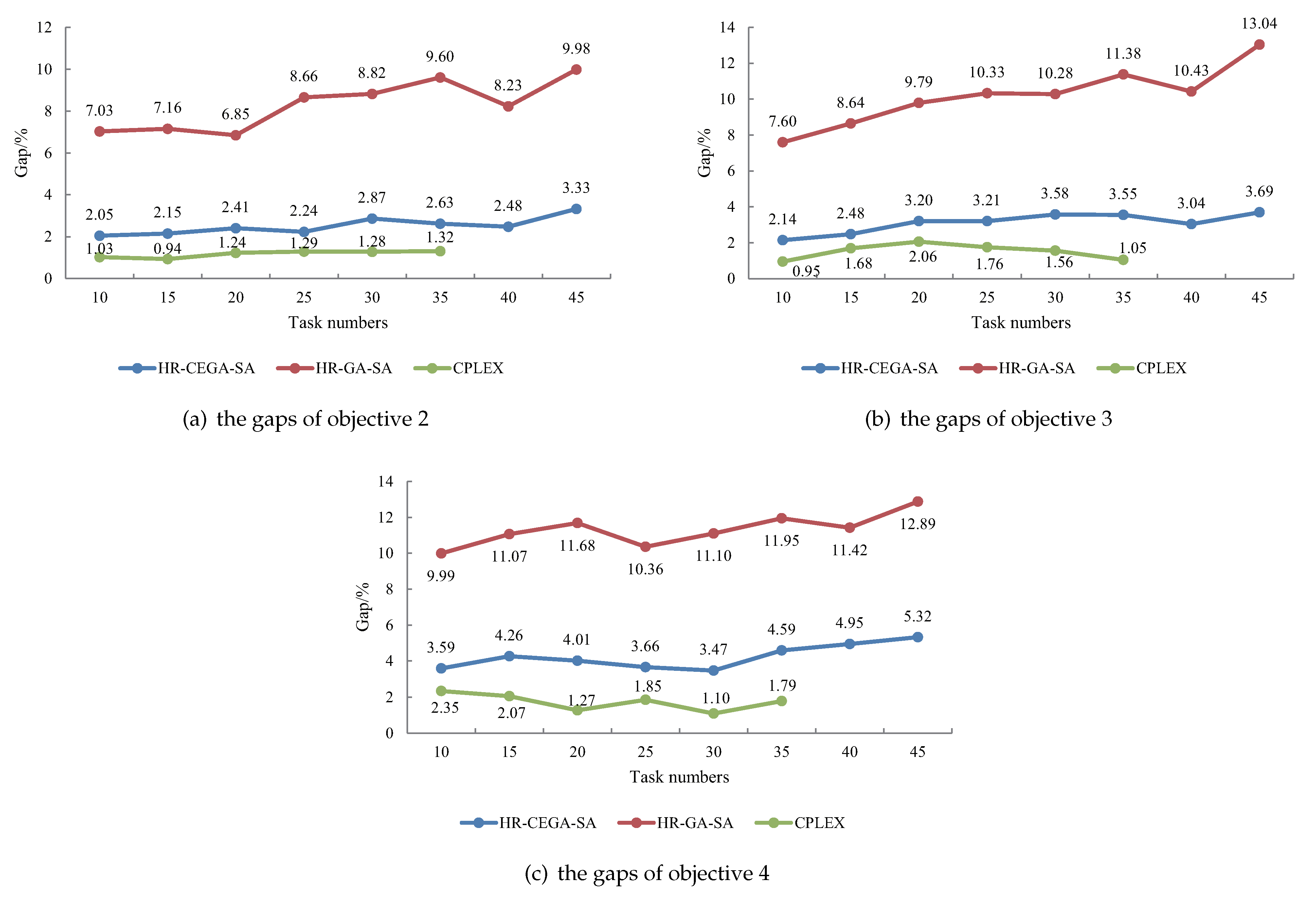
Gap is introduced to evaluate the difference among four algorithms, as shown in Figure 13. The calculation of gap for objectives is shown in Equation (57). The average gaps of Objectives 2–4 obtained from HR-ECEGA-SA and CPLEX are very small: 1.18%, 1.51%, and 1.73%, respectively. The average gaps of Objectives 2–4 obtained from HR-ECEGA-SA and HR-GA-SA are the largest: 8.29%, 10.18%, and 11.31% respectively. Compared to CEGA, EGECA makes full use of the elite individual to improve the average performance of solutions by 2.52%, 3.11%, and 4.23%, respectively. Therefore, the validity of HR-ECEGE-SA is verified.

$$Gap=\frac{\left({\Phi }_{ij}^1-{\Phi }_{i1}^1\right)\ast 100}{{\Phi }_{i1}^1},\forall i=\{2,3,4\},j=\{1,2,3,4\}$$

(57)

where ${\Phi }_{ij}^1$ means $Z_i$, that is, the value of objective i for algorithm j. If the algorithm is HR-ECEGA-SA, $j=1$; if the algorithm is HR-CEGA-SA, $j=2$; if the algorithm is HR-GA-SA, $j=3$; and if the algorithm is CPLEX, $j=4$.

4.4. Numerical Experiments with Different Division Rules of Crane Area

To verify the superiority and universality of the crossing crane area, we compared the results of four division strategies at different task numbers: the dynamic crossing crane area (DM1) that we propose, three-equivalent cross crane area (DM2) used for the initialization described in Section 3.1, disjunctive crane area equally (DM3) [7,8], and static disjunctive crane area (DM4) [30,31,32,36]. In Figure 14, the gaps are the objective differences between the DM1 and DM2, as well as between DM3, and DM4.

In Figure 14, firstly, the balance rates of DM1 of each instance are greater than 90%, and the maximum average value is 97.48%. However, the balance rates of three traditional strategies, that is DM2, DM2, and DM4, do not have satisfactory values. Gap is introduced to evaluate the difference among the four division rules, which is calculation using Equation (58). The gap of four division rules can be observed in Figure 14. Compared to other division rules, the average gaps of Objective 1 obtained from DM1 are 17.05%, 37.25%, and 37.10%, respectively. Then, the average makespan, handling cost, and energy consumption obtained from DM1 are the smallest. In contrast with DM2, DM3, and DM4, DM1 can reduce the average makespan by 4.37%, 9.87%, and 7.54%, respectively; reduce the average handling cost by 5.36%, 9.37%, and 7.40%, respectively; and decrease the average energy consumption by 6.99%, 6.97%, and 6.23%, respectively. DM1 comprehensively considers the flexibility of crane area unlike DM2. The specific location of tasks is ignored in DM3. The empty-loaded movement is ignored in DM4 as well as full-loaded movement of GCs. Besides, DM1 based on the handling plan of “GCs-ITs” reduces energy consumption because the long-distance movement of GCs is replaced by ITs. Therefore, we can prove the effectiveness and excellence of DM1, namely the crossing crane area we proposed.

$$Gap-DMj=\frac{\left({\Phi }_{ij}^2-{\Phi }_{i1}^2\right)\ast 100}{{\Phi }_{i1}^2},\forall i=\{1,2,3,4\},j=\{2,3,4\}$$

(58)

where ${\Phi }_{ij}^2$ means $Z_i$, that is, the value of objective i for the division rule j. If the rule is DM1, $j=1$; if the rule is DM2, $j=2$; if the rule is DM3, $j=3$; and if the rule is DM4, $j=4$.

4.5. Sensitively Analysis

4.5.1. Sensitively Analysis with IT Number

As depicted above, compared with GCs, ITs have higher flexibility, faster speed, lower energy consumption, and lower operating costs. Therefore, deciding the numbers of ITs reasonably is vital for the RCT. We compare the results of one instance shown in Table 2 under various IT configurations.

In

Table 6. The results of different number of the ITs.

IT Numbers	${\mathit{Z}}_1$	${\mathit{Z}}_2$	${\mathit{Z}}_3$	${\mathit{Z}}_4$	GAP of ${\mathit{Z}}_2$	GAP of ${\mathit{Z}}_3$
1	infeasible	infeasible	infeasible	infeasible	—	—
2	94.10	3769.35	1647.62	213.97	—	—
3	95.9	3368.09	1459.69	210.10	10.64%	11.41%
4	97.21	3186.46	1368.71	212.79	5.39%	6.23%
5	97.05	3091.75	1327.65	205.93	2.97%	3.00%
6	94.39	3036.62	1315.21	216.88	1.78%	0.94%
7	97.17	3031.85	1318.05	210.81	0.16%	−0.22%

, the balance rates of each instance meets the satisfaction value of 90%. The number of ITs mainly affects the makespan and handling cost. We calculate the gap of makespan and handling cost using Equation (59).

$$Gapof{Z}_i=\frac{({\Phi }_{ij}^3-{\Phi }_{ij-1}^3)\ast 100}{{\Phi }_{ij-1}^3},\forall i=\{2,4\},j=\{3,4,5,6,7\}$$

(59)

where ${\Phi }_{ij}^3$ means $Z_i$, that is, the value of objective i for the IT number j. If the number is 3, $j=3$; if the number is 4, $j=4$; etc.

In Table 6, the handling requirements cannot be met when the number of ITs is 1, resulting in infeasible for the integrated optimized problem. When the number of ITs is fewer, the operation efficiency is poorer and the handling cost is higher. However, the startup cost of ITs is increasing with the increase in the number of ITs. In general, with the increase in the number of ITs, the improving trend of efficiency and the decreasing trend of cost gradually slows. When the number of ITs increases from 2 to 3, the makespan and cost decreases most obviously, up to 10.64% and 11.41%, respectively. If the value is greater than 6, there may be idle ITs, which would not join in handling operation.

Thus, RCT can rationalize the number of ITs according to operational needs. Table 6 can be used as a reference basis. If RCT pays more attention to operational benefits and efficiency, three ITs can be configured. If it is limited by IT resources and startup cost of the IT, the optional configuration is 4. The results prove that the model and algorithm designed in our paper are effective and stable for different number of ITs.

4.5.2. Sensitively Analysis with Stopping Position of the Train

When the start and target slots of tasks are known, the stopping position of the train affects the moving distance of handling equipment between each task, which in turn affects the division of the crossing crane area and each objective above. Thus, for sensitivity analysis, a comparison experiment with different stopping position of the train was performed. The stopping position corresponds to the first bay of the yard. Therefore, in Figure 15, the value of stopping position equals the serial number of the first bay.

In Figure 15, the average balance rates of each stopping position meet the satisfactory value of 90%, and the largest is 98.64%. As the stopping position varies from 1 to 10, the trend of the makespan, handling cost, and energy consumption are to decrease first and then increase. The lower is the stopping position, the farther away is the rear of the train from the yard. The higher is the parking position, the farther away is the headstock from the yard. In all tests, these objectives are minimum when the stopping position is 5, and the differences with the values of 4 and 6 are small. Hence, the stopping position of the train should be reasonably determined according to the position of the tasks in the train and yard to improve the handling performance. In our case, values of 4–6 are recommended, by which the handling efficiency and cost can be improved, while the energy consumption be reduced.

5. Conclusions

In this paper, the integrated allocation and scheduling of handling resources in the RCT are discussed. To improve the handling efficiency and reduce the handling cost and energy consumption, we propose the new handling scheme of “GCs-ITs”, generating two handling modes: direct move and split move. In the latter, the IT is applied to replace the long-distance, full-loaded movement of GC. We decompose the integrated optimization problem into four sub-problems: yard partition, crane assignment, crane scheduling, and IT scheduling. Considering outbound containers, a multi-objective MIP model is developed. Analyzing the characteristics of the problem, we designed a TLHHA incorporating HR, ECEGA, GA, and SA to obtain the solution. Furthermore, the effectiveness of the model and algorithm is verified by analyzing and comparing the experimental results under different optimization algorithms and division rules for crane area. Besides, we investigate the sensitive analysis considering IT numbers and the stopping position of the train. Our research has the following conclusions.

• The moving distance of GC applied to measure the workload is more reasonable in reflecting the handling performance. Due to the simultaneous consideration of the container’s position, the full-loaded and empty-loaded of dual-GC, and the flexibility of crane area, the principle of dynamic crossing crane area that we propose has the highest balance rate compared to the three traditional principles.
• Based on the “GCs-ITs” scheme, we take advantage of IT to make up for the disadvantage of GC. Therefore, the integrated optimization problem has better efficiency, benefit, and energy-saving.
• The ECEGA that we propose in the second-layer of the TLHHA can speed up the convergence, avoid premature convergence, and ensure the global optimal solution. According to the results of experiments, the solving efficiency and performance of HR-ECEGA-SA can be validated by comparing it to HR-CEGA-SA, HR-GA-SA, and CPPLEX.
• The number of ITs mainly affects the makespan and handling cost of the RCT. Too few ITs cannot meet the handling requirements, and too many will undoubtedly increase the construction cost of RCT. For our case, the optimal configuration is 3.
• The stopping position of the train affects the moving distance of handling equipment. By experiments, we verify that the stopping position should be selected so that the center of the train is close to the center of the yard. For the instance of our research, the optimal stopping position is 5.

This research still has some limitations. We did not consider the congestion of the ITs in the handling area and the storage slot allocation. For future study, these two factors should be further explored. Another challenge is to simultaneously optimize integrated allocation and scheduling problems for the outbound and inbound containers stored in the yard and external trucks of the rail-road railway terminal. Finally, we consider the handling plan of “GCs-ITs”. However, the handling equipment varies different RCT. Therefore, the different handling plans can be evaluated from the perspective of operation cost (including construction cost and handling cost), handling effectively, and environmental protection in future research. The various handling plan includes GCs, “GCs-ITs”, RSs, and “GCs-RSs”.

References

- Boysen, N.; Fliedner, M.; Jaehn, F.; Pesch, E. A survey on container processing in railway yards. Trans. Sci. 2013, 47, 312–329. [Google Scholar] [CrossRef]
- Guo, P.; Cheng, W.; Zhang, Z.; Zhang, M.; Liang, J. Gantry crane scheduling with interference constraints in railway container terminals. Int. J. Comput. Intell. Syst. 2013, 6, 244–260. [Google Scholar] [CrossRef] [Green Version]
- Guo, P.; Cheng, W.; Wang, Y.; Boysen, N. Gantry crane scheduling in intermodal rail—road container terminal. Int. J. Prod. Res. 2018, 56, 5419–5436. [Google Scholar] [CrossRef]
- Chang, Y.; Zhu, X.; Yan, B.; Wang, L. Integrated scheduling of handling operations in railway container terminals. Trans. Lett. Int. J. Trans. Res. 2019, 11, 402–412. [Google Scholar] [CrossRef]
- Chang, Y.; Zhu, X.; Haghani, A. Modeling and solution of joint storage space allocation and handling operation for outbound containers in rail-water intermodal container terminals. IEEE Access 2019, 7, 55142–55158. [Google Scholar] [CrossRef]
- Zeng, M.; Cheng, W.; Guo, P. Modelling and metaheuristic for gantry crane scheduling and storage space allocation problem in railway container terminals. Discrete Dyn. Nat. Soc. 2017, 2017, 1–13. [Google Scholar] [CrossRef] [Green Version]
- Wang, L.; Zhu, X. Rail mounted gantry crane scheduling optimization in railway container terminal based on hybrid handling mode. Comput. Intell. Neurosc. 2014, 2014, 1–8. [Google Scholar] [CrossRef] [PubMed]
- Wang, L.; Zhu, X. Container loading optimization in rail-truck intermodal terminals considering energy consumption. Sustainability 2019, 11, 2383. [Google Scholar] [CrossRef] [Green Version]
- Shi, X.; Voß, S. Container terminal operations under the influence of shipping alliances. In Risk Management in Port Operations, Logistics and Supply Chain Security; Bichou, K., Bell, M.G.H., Evans, A., Eds.; Informa: London, UK, 2007; pp. 135–167. [Google Scholar]
- Boysen, N.; Briskorn, D.; Meisel, F. A generalized classification scheme for crane scheduling with interference. Eur. J. Oper. Res. 2017, 258, 343–357. [Google Scholar] [CrossRef]
- Kizilay, D.; Eliiyi, D.T. A comprehensive review of quay crane scheduling, yard operations and integrations thereof in container terminals. Flexible Serv. Manuf. J. 2020, 2020, 1–42. [Google Scholar] [CrossRef]
- Hu, L.; Shi, X.; Voß, S.; Zhang, W. Application of RFID technology at the entrance gate of container terminals. In International Conference on Computational Logistics; Springer: Berlin/Heidelberg, Germany, 2011; Volume 6971, pp. 209–220. [Google Scholar]
- Shi, X.; Tao, D.; Voß, S. RFID technology and its application to port-based container logistics. J. Organ. Comput. Electr. Commerce 2011, 21, 332–347. [Google Scholar] [CrossRef]
- Shi, X.; Vanelslander, T. Design and evaluation of transportation networks: Constructing transportation networks from perspectives of service integration, infrastructure investment and information system implementation. Netnomics 2010, 11, 1–4. [Google Scholar] [CrossRef] [Green Version]
- Zheng, F.; Man, X.; Chu, F.; Liu, M.; Chu, C. Two yard crane scheduling with dynamic processing time and interference. IEEE Trans. Intell. Transp. Syst. 2018, 19, 3775–3784. [Google Scholar] [CrossRef]
- He, J.; Tan, C.; Zhang, Y. Yard crane scheduling problem in a container terminal considering risk caused by uncertainty. Adv. Eng. Inf. 2019, 39, 14–24. [Google Scholar] [CrossRef]
- Kaveshgar, N.; Huynh, N. Integrated quay crane and yard truck scheduling for unloading inbound containers. Int. J. Prod. Econ. 2015, 159, 168–177. [Google Scholar] [CrossRef]
- Zhen, L.; Yu, S.; Wang, S.; Sun, Z. Scheduling quay cranes and yard trucks for unloading operations in container ports. Ann. Oper. Res. 2019, 273, 455–478. [Google Scholar] [CrossRef]
- Bierwirth, C.; Meisel, F. A fast heuristic for quay crane scheduling with interference constraints. J. Schedul. 2009, 12, 345–360. [Google Scholar] [CrossRef]
- Bian, Z.; Xu, Q.; Li, N.; Jin, Z. Scheduling for yard crane based on two-stage hybrid dynamic programming. Transport 2018, 33, 408–417. [Google Scholar] [CrossRef] [Green Version]
- Chen, L.; Langevin, A.; Lu, Z. Integrated scheduling of crane handling and truck transportation in a maritime container terminal. Eur. J. Oper. Res. 2013, 225, 142–152. [Google Scholar] [CrossRef]
- Yu, K.; Yang, J. MILP model and a rolling horizon algorithm for crane scheduling in a hybrid storage container terminal. Math. Probl. Eng. 2019, 2019, 1–16. [Google Scholar] [CrossRef] [Green Version]
- Facchini, F.; Boenzi, F.; Digiesi, S.; Mummolo, G. A model-based Decision Support System for multiple container terminals hub management. Prod. J. 2018, 28, 1–12. [Google Scholar] [CrossRef]
- Facchini, F.; Digiesi, S.; Mossa, G. Optimal dry port configuration for container terminals: A non-linear model for sustainable decision making. Int. J. Prod. Econ. 2020, 219, 161–178. [Google Scholar] [CrossRef]
- He, J.; Huang, Y.; Yan, W.; Wang, S. Integrated internal truck, yard crane and quay crane scheduling in a container terminal considering energy consumption. Expert Syst. Appl. 2015, 42, 2464–2487. [Google Scholar] [CrossRef]
- Boysen, N.; Scholl, J.; Stephan, K. When road trains supply freight trains: Scheduling the container loading process by gantry crane between multi-trailer trucks and freight trains. OR Spectrum 2017, 39, 137–164. [Google Scholar] [CrossRef]
- Tschoeke, M.; Boysen, N. Container supply with multi-trailer trucks: Parking strategies to speed up the gantry crane-based loading of freight trains in rail yards. OR Spectrum 2018, 40, 319–339. [Google Scholar] [CrossRef]
- Yang, Y.; Zhu, X.; Haghani, A. Multiple equipment integrated scheduling and storage space allocation in rail-water intermodal container terminals considering energy efficiency. Trans. Res. Record 2019, 2673, 199–209. [Google Scholar] [CrossRef]
- Yue, L.; Fan, H.; Zhai, C. Joint configuration and scheduling optimization of a dual-trolley quay crane and automatic guided vehicles with consideration of vessel stability. Sustainability 2020, 12, 1–16. [Google Scholar]
- Boysen, N.; Fliedner, M.; Kellner, M. Determining fixed crane areas in rail-rail transshipment yards. Trans. Res. Part E-Logist. Transp. Rev. 2010, 46, 1005–1016. [Google Scholar] [CrossRef] [Green Version]
- Boysen, N.; Filedner, M. Determining crane areas in intermodal transshipment yards: The yard partition problem. Eur. J. Oper. Res. 2010, 204, 336–342. [Google Scholar] [CrossRef] [Green Version]
- Boysen, N.; Emde, S.; Fliedner, M. Determining crane areas for balancing workload among interfering and noninterfering cranes. Sustainability 2012, 59, 656–662. [Google Scholar] [CrossRef]
- Fan, H.; Yao, Q.; Ma, M. Storage space allocation based on regional workload balance planning of multiple yard cranes in container terminal yard. Control Dec. 2016, 31, 1603–1608. [Google Scholar]
- Fan, H.; Ma, M.; Yao, Q.; Guo, Z. Integrated optimization of storage space allocation and multiple yard cranes scheduling in a container terminal yard. J. Shanghai Jiaotong Univ. 2017, 51, 1367–1373. [Google Scholar]
- Tang, L.; Guo, P. Study of loading/unloading equipment optimization scheduling in railway container terminal. Comput. Eng. Appl. 2012, 48, 211–214. [Google Scholar]
- Fedtke, S.; Boysen, N. Gantry crane and shuttle car scheduling in modern rail–rail transshipment yards. OR Spectrum 2017, 39, 473–503. [Google Scholar] [CrossRef]
- Fedtke, S.; Boysen, N. A comparison of different container sorting systems in modern rail-rail transshipment yards. Trans. Res. Part C-Emerg. Technol. 2017, 82, 63–87. [Google Scholar] [CrossRef]
- Wang, X.; Lian, K.; Zhang, H.; Jin, Z. Dynamic gantry crane allocation and integrated scheduling with truck in the railway container terminal. Comput. Integr. Manuf. Syst. 2020, 2020, 1–18. [Google Scholar]
- Wang, X.; Jia, Y.; Cai, J.; Jin, Z. Integrating optimization of resource allocation and handling scheduling in railway container terminal. Control Dec. 2020, 2020, 1–10. [Google Scholar]
Figure 1.
The layout of RCT.
Figure 2.
An example of the DRCT equipped with GCs.
Figure 3.
Two handling mode in main storage yard.
Figure 4.
Algorithm design for integrated scheduling problem.
Figure 5.
Flowchart of the proposed TLHHA.