
Simulation of Railway Lines with a Simplified Interlocking System


1
Faculty of Transport Engineering, University of Pardubice, 532 10 Pardubice, Czech Republic
2
Faculty of Operation and Economics of Transport and Communications, University of Žilina, 010 26 Žilina, Slovakia
*
Author to whom correspondence should be addressed.
Sustainability 2021, 13(3), 1394; https://0-doi-org.brum.beds.ac.uk/10.3390/su13031394
Submission received: 7 December 2020
/
Revised: 26 January 2021
/
Accepted: 26 January 2021
/
Published: 29 January 2021
(This article belongs to the Special Issue Innovative and Sustainable Management of International Shipment Flow: Opportunities and Challenges)
Abstract
:This paper deals with railway lines with low traffic intensity where trains are operated under simplified conditions. Those conditions are stated in a regulation, and there is no interlocking system on the line. The whole railway operation is organized according to a regulation in cooperation with the train crew. For the calculation of the throughput, we can use analytic or simulation methods. On those lines there is a big problem with the common working methods because of special circumstances on each line, which are influencing the technological times and reliability of the calculation. The simplified conditions are the transforming of regular interlocking systems on the administrative level. Therefore, it is very complicated to use a common simulation model. Most of the simulation tools are not able to work with it. The motivation of this paper is to prove that modern simulation tools are usable for that specific condition as well. The simulation model was built in SW OpenTrack which is able to modify its functions to figure out each technological action to ensure the correct function of the model. This functionality is described in the paper in general and implemented on a case study.
1. Introduction
Simulation modeling is one of the tools for assessing capacity (throughput performance), traffic efficiency, and reliability on railway lines. These indicators can be successfully followed and assessed on lines with actual traffic requirements approaching the capacity limits of the infrastructure. There are national and international regulations [1,2,3,4,5], which contain a mathematic apparatus for the assessment of the capacity of lines, line tracks, station point areas (heads) and station tracks, or for the assessment of the stability of the timetable. These tracks or parts of the infrastructure are also very often successfully simulated in various simulation tools.
On the other hand, there are many regional lines or light rails where the operation is regulated by special traffic regulations without any interlocking system. They are usually simpler, and hence they are called lines with a simplified method of train operation. In the Czech Republic, the SŽDC D3 [6] regulation sets out internal rules for the operation of such lines. The method of operation is usually simplified for cost-saving reasons; certain duties of employees of the railway infrastructure manager are taken over by employees of the railway. A significant disadvantage of that regulation [7] is the fact that we are not able to simulate it using simulation tools in basic settings. A method needs to be discovered to simulate the conditions of regional lines in a simulation tool. The authors use the simulation tool OpenTrack, but the method should be applicable universally.
This modified method should calculate operating intervals, headways, or capacity indicators as required by the main regulations for capacity assessment, but considering specific local requirements. On the other hand, the users should consider local specifics, because each system of simplified interlocking and means of operation can possibly be specific (especially if the simulated railway lines are located in different countries). Some differences can also be found between lines with simplified operations within one railway network (country).
The customary examples of differences between classic and simplified lines are the different methods of communication between traffic crew and the different methods of manipulation with points. This leads to specific situations in train operation, e.g., trains must sometimes also stop at station point areas due to manipulation with points, or some technological times can be extended due to the specific obligations of a crew. These effects are usually impossible to simulate.
The advantage of simulation is the fact that the model can fully include all specific operating intervals for each variant of the possible routes of all trains. If designed correctly, such a model can provide a truly sound examination of all possible operating scenarios on the line. This approach can help make these lines more attractive for passengers as well as freight transport.
The last section of this paper also compares different interlocking systems on one line from the period and timetable stability points of view.
2. Literature Review
The capacity problem of the lines with low traffic intensity are only solved by scientific teams rarely. The reason is that the capacity of such lines is not often a bottleneck from the quantitative point of view; however, qualitative aspects of capacity are also taken into consideration these days. Additionally, lines without any interlocking are not a frequent subject of scientific papers, but the significance of those lines for public service might be high. This is the reason why it is necessary to also provide for the simulation of such lines, making it possible to assess the operational stability, the application of a periodic timetable, and similar qualitative effects.
There are some articles which solve this problem from the capacity point of view [8,9,10,11], the economic point of view [12,13], or the strategic point of view [14,15]. But none of those articles addresses the possibility of simulating those regional lines with simplified train operational control in a simulation tool. Simulation is a very modern and progressive method for timetable preparation or stability evaluation. Railway infrastructure capacity is currently mostly assessed using the UIC code 406 [3,4]; in the Czech Republic, capacity is also calculated based on the SŽDC SM 124 [7] guideline or the SŽDC (ČD) D24 [2] methodology regulation (this methodology is generally used in Slovakia as well) [1,2]. The new regulation SŽDC SM 124 [7] is basically a genesis of the original guideline SŽDC (ČD) D24 [2], which implements some parts of the UIC 406 [3] in Czech conditions. The following Equation (1) is used to determine capacity in the Czech Republic:
where
- n = number of trains (trains)
- s = occupancy ratio (–)
- T = calculation time (1440 min or a peak period) (min)
- b = average time of occupation (min)
The maximum value of the occupancy ratio is 0.62 [7]. Above this value, a system is overloaded. From Equations (1) and (2) can be derived for the maximum transportation capacity. This method primarily uses the number of trains during a calculation period.
where
- nopt = optimal value of transportation capacity (–)
- smax = maximum value of occupancy ratio (–)
The degree of occupancy (S) is also a very important index used for scoring the quality [Sm 124]. It can be calculated using Equation (3).
where
- S = occupancy ratio (–)
- bi = occupation time for train i (min)
The UIC 406 methodology uses capacity consumption expressed as a percentage, assuming that capacity as such does not exist. Capacity consumption is calculated using Equation (4).
where
- CC = capacity consumption (%)
- OT = occupancy time (min)
- AT = additional time (min)
- ATR = additional time rate (%)
- DTP = defined time period (min)
Each methodology has its advantages and disadvantages. The regulation UIC 406 methodology is for instance more suitable for line sections with essentially stable transport intensity and traffic volume [3]. By contrast, the SŽDC SM 124 guideline is more precise in expressing the used capacity as a percentage of the total daily calculation time for each block section (interstation section). Both of those methods are usable also for lines with low traffic intensity.
Another group of scientific papers deals with determining traffic efficiency [8,16,17]. However, these only compare the railway line capacity indicators before and after the modernization of railway infrastructure. The actual process of traffic optimization on these lines is not described anywhere and the possibilities of train operation simulation are only described briefly [18,19]. It is only the demographic factors influencing the demand for public transport that are mostly considered [20]. Another paper deals with the technology providing for a comprehensive assessment of the quality of services provided in regional rail passenger transport. The proposed quality assessment methodology can be used for comparing integrated transport systems based on their quality, and it can serve to assess the services provided in relation to either the contracting authority or the provider. The methodology adopts the EU transport policy in full [11]. The increase in the performance of rail passenger and freight transport increases the efficiency of a regional railway line, but the ratio between the passenger and freight transport on a regional railway line influences the government budget requirements [21]. Ref. [12] compares the development in the performance of freight and passenger transport on a regional railway line, proposing measures for regional rail transport in a region with different suspected economic potential, which would be reflected in the efficient use of public funds. The authors [22] deal with connecting regional, national, and local railways. For the purposes of that research, a model of the current and future situations was created. Based on the simulation model, several variants of the operation of new passenger trains under new conditions were proposed and analyzed. This study served as a basis for connecting national and regional lines in Croatia. The same was true for Ref. [23], which dealt with setting railway infrastructure fees on regional railways.
Additionally, Ref. [12] deals with transport planning on regional railways. The authors assume that successful transport planning must be based on as accurate as possible a description of passenger flows, including parameters influencing the choice of the mode of transport. These inputs represent a substantial base for the following steps: creating a track network, proposing a timetable, managing vehicle rosters and employee courses, managing infrastructure improvements and related requests. There are currently only a few transport models in the Czech Republic providing for relevant outputs for public service transport planning. That is why the authors used different heuristics, one of which is illustrated by a practical example: transforming the timetable concept on a selected railway network, including the effects of changes in the number of passengers.
The authors [24,25,26] deal with the quality assurance of traffic on regional railway lines from the perspectives of passengers, railway undertakings and transport operators. Their papers focus on assessing the quality of performance in regional rail passenger transport compared to other public transport modes. In this respect, it is necessary to examine the perception of the quality of the services and their value for clients (passengers) in scientific terms as well. The main aspects of the quality of transport services in this sense are the vehicles and the transport infrastructure. It is therefore necessary to establish a permanent process of quality assessment for the transport services provided. The papers assume that the interests of customers are represented by the public contracting authority in public transport services.
Traffic modeling on railway lines with different traffic volumes is described in Refs. [27,28]. This literature uses a simulation as an intermediate step to view the characteristics of the whole transport system. The methods mentioned therein are aiming at goals such as use of transport infrastructure, traffic simulation for considering energy consumption, or the creation of a timetable and assessing its stability. All the above-mentioned models consider technological, technical, or economic perspectives. However, as for the transport volume, the respective lines correspond to national or regional railway lines. A complex solution for railway lines with low and specific traffic, as presented in our paper, is only touched upon there very briefly.
The model in this study is focused on a more detailed microscopic model of traffic on lines with low traffic intensity. Unlike the above-mentioned scientific studies, it discusses the individual steps of model creation, simulation and evaluation.
The objective of this paper is different. The method fills in the gap in the research, because it is focused on the comparison of different transport technologies on the lines with low intensity. It is a scientific challenge to set up a simulation tool to simulate lines with low traffic intensity faithfully.
3. General Simulation Model
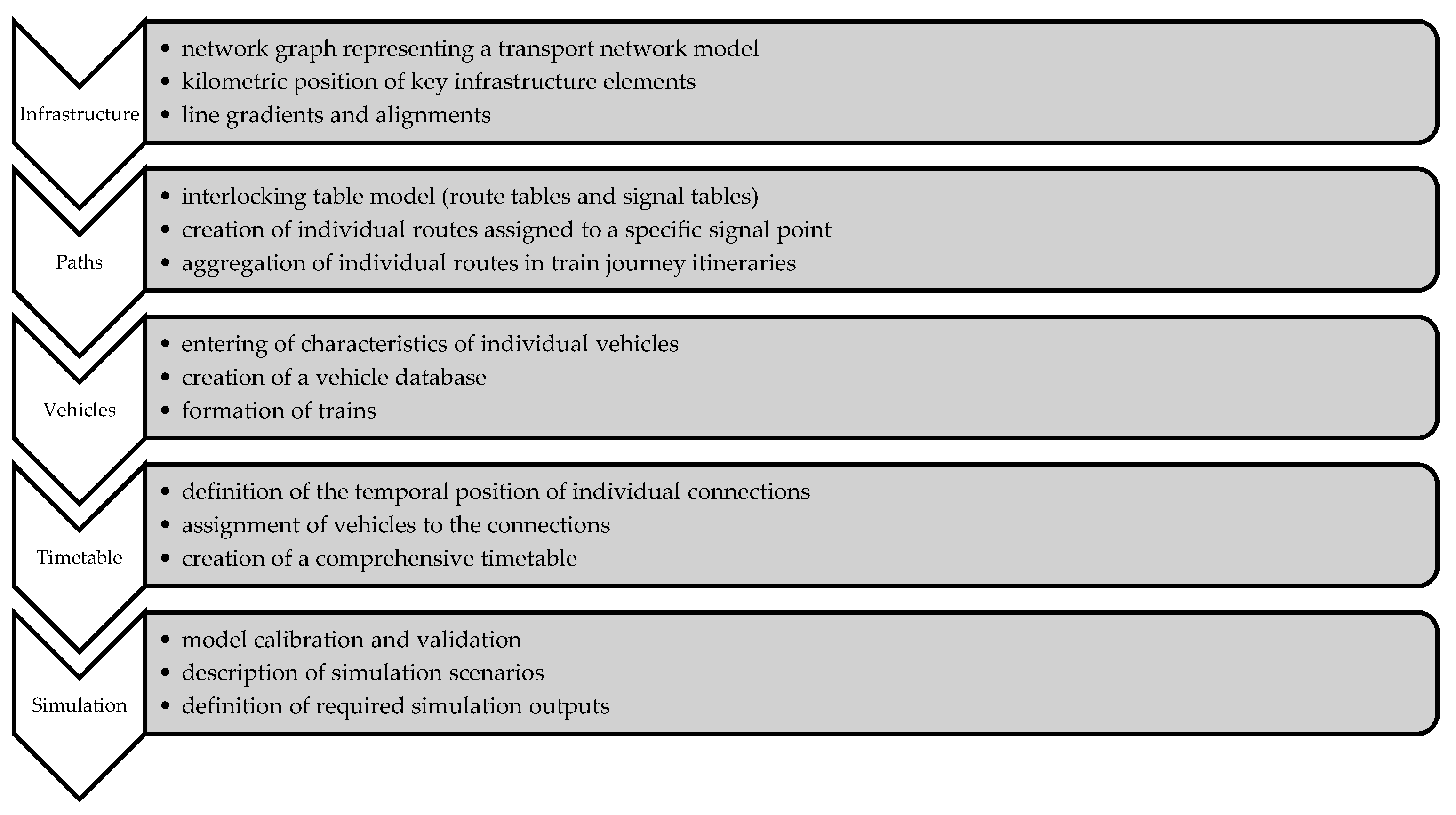
This section describes a general procedure for creating a simulation model in OpenTrack, which authors use as a simulation tool. The model is prepared in five distinct stages, as described in Figure 1. This general procedure is further modified to reflect a model of a line with low traffic intensity and simplified transport control.
The network graph representing a transport network model is based on the known gradient and alignment characteristics of the railway line. Furthermore, all permitted routes must be entered in the transport network model. A route always begins and ends at a signal point. In the standard simulation model, the line section is released after releasing the last point on the route. The releasing time depends on the interlocking or signaling systems in the station. On lines with low traffic intensity with no signaling systems, it is necessary to come up with a different solution, because signals are replaced by a system of communication between the train crew and a dispatcher.
3.1. Basic Idea of the Research
The authors used a regulation [6] which is applied on lines with low traffic intensity, and invented a procedure for the software model adjustment. The idea is to create fictitious signal points on both station heads, so that one station will be split into three substations. Where there is no signaling system and all routes are set by a member of the train crew manually, it is necessary to ensure that a train heading to another track than the one given by the primary position of the point stops before the outer point. This condition also needs to be met when a train enters an unoccupied operating area as second [29,30]. Before the outer points in the model, it is therefore necessary to insert a fictitious operating point where the train would stop for a specified time period, simulating the time necessary for route preparation in actual traffic. Furthermore, it is to be ensured that the block condition is met [31,32]. This means that a train cannot leave the previous operating point until the dispatcher controlling the line traffic is notified of the arrival of the first train. That is why, as in reality, the model does not include home signals [33]. In these cases, the route is defined by the exit signal of the first operating point and the starting signal of the second operating point. For every route, the time periods for route preparation and releasing need to be defined. These periods are specific for each operating point and are calculated based on defined technological times. Figure 2 shows a diagram of route creation on railway lines with low traffic intensity. This idea is also applicable for stations with group signal points [34]. In such cases, one signal is valid for all the station tracks, and train drivers must also follow the additional information provided by the dispatcher when there are more trains at the same time.
3.2. Theoretic Example
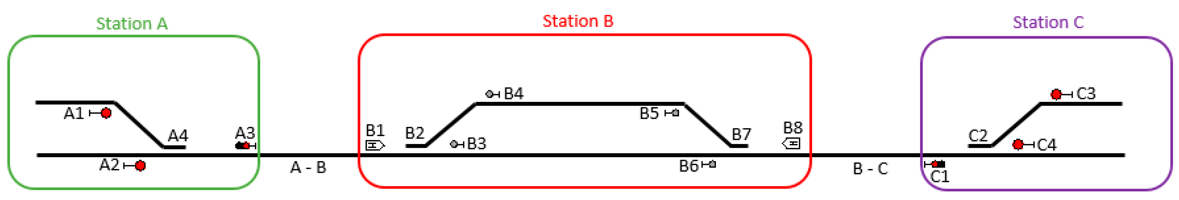
Figure 2 shows three stations, with stations A and C being controlled by a dispatcher directly operating the signaling systems. Station B and adjacent interstation sections are not equipped with a signaling system and are not directly controlled by an employee controlling the rail transport. A member of the train crew is directly involved in the preparation, informing the dispatcher of the position of their train, its integrity, and the position of the points. That is why, for instance, the route from signal A2 to signal B6 can be released once the locomotive driver announces their arrival by telephone. In the route from signal C3 to signal B4, it is necessary to stop at point B8 and reset point B7. The subsequent notification process is the same. In general, a point is reset by a member of the train crew crossing it first, who then sets it back to the primary position after the train ride. This means that if the route goes from signal B4 or B5, the time needed for manual point resetting is included in the route preparation time. The train then must stop at fictitious operating points B1 or B8, and its stay there simulates the time needed for manual point resetting by a member of the train crew. As for routes from station B to stations A or C, a route can be released once the locomotive driver stops and announces the integrity of the train and their leaving the railway line. These time periods again need to be calculated individually for each station. A precise setting of routes and their mutual dependencies is vital for observing station and line intervals. The routes created are then used to compile a train journey itinerary defining all routes that the respective train or group of trains can use.
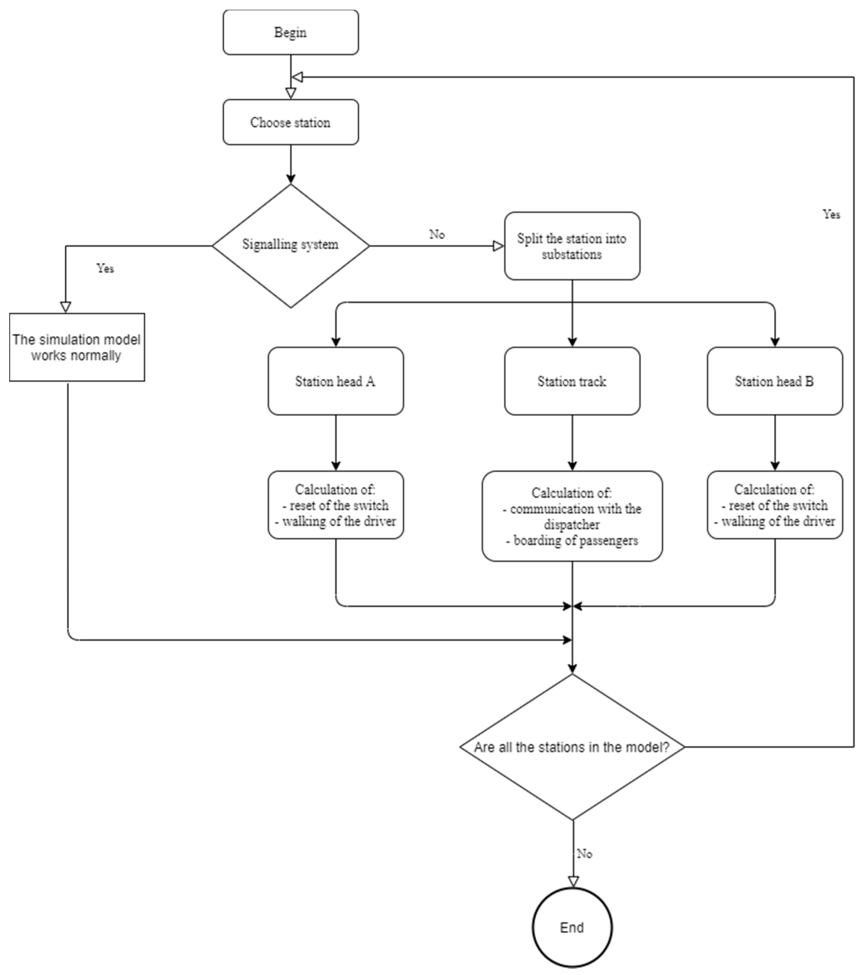
Another difference compared to a conventional rail traffic model lies in the different lengths of journey times for the same train types, depending on whether a member of the train crew must prepare the route. These journey time extensions need to be calculated and considered in creating the timetable. The process of the model preparation suggested within our research is shown in Figure 3.
4. Case Studies on the Moravany–Borohrádek Line
This paper includes a case study of operation on the line Moravany–Holice–Borohrádek on the border of the Hradec Králové and Pardubice Regions. Based on the model of this line, the principles of simplified train operation control in the Czech Republic are explained. Furthermore, the traffic is simulated, and the simulation is calibrated and validated.
The same line section of Moravany–Holice–Borohrádek was also selected for a parallel case study to test the influence of the signaling system on the timetable stability and its ability to compensate for delay. The investigated line section is 17.137 km long. The maximum line speed is 60 km·h−1 (with local speed limitations). There are three stations located in this section, as can be seen from the simplified presentation in Figure 2. The Moravany station (Station A) is controlled using a remotely controlled electronic signaling system. The Borohrádek station (Station C) is equipped with a mechanical interlocking machine controlled locally. The Holice station (Station B) located in the middle of the section considered is not equipped with a station signaling system and the adjacent sections are not equipped with any trackside signaling system. In the Holice station and the adjacent line sections, the traffic is controlled in accordance with a special transport regulation [6] governing lines with simplified train operation control. Train and shunting routes are prepared manually by a member of the train crew based on the instructions of the dispatcher communicated through the radio network.
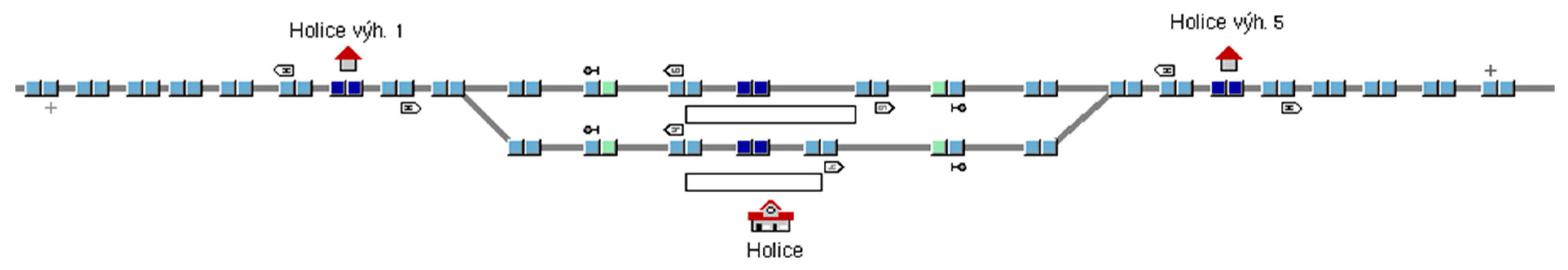
The first part of the case study uses simulation to focus on establishing operating intervals (crossing of trains or successive intervals), headways, and other indicators. Figure 4 shows part of a worksheet used to simulate the Holice station. The study first assesses the present state and then the impact of the proposed measures. Proposed are modifications from the non-existent interlocking system to the modern signaling system. In the first case, points at the Holice station are replaced by resetting trailable points. In the second case, the Holice station and the adjacent interstation sections are equipped with an electronic trackside and station signaling system, so that the most important task is to determine if the points are operated locally or remotely.
Currently (as of timeTable 2019/2020), the line is served by two types of passenger diesel motor units, Class ČD 810 or 814. Locomotive Class 742 is used for freight trains. The parameters of the individual vehicles are provided for in Table 1.
4.1. Journey Times and Model Calibration
An integral part of the preparation of a simulation model is its calibration and the verification of its functioning. The first step in creating the main part of the infrastructure model, a partial database of routes, and transit itineraries is the verification of journey times. Ideally, these are verified using a tachograph from an actual traction railway vehicle. This was explored, for instance by the author of Ref. [29], who in his paper establishes vehicle running resistance using statistical examination to validate the model’s values. Where no data are available, it is possible to compare the journey times to known journey times established in creating the train diagram. A comparison of journey times is provided in Table 2. For the purposes of comparison with actual traffic data, it will be necessary to obtain data from the on-board unit of a vehicle on the railway line considered, which will allow for the even more precise comparison and calibration of the simulation model. Journey times which could not be established from the timetable created were calculated based on the simulation results, and rounded to the nearest half minute. These are the journey times of passenger trains between Holice and Borohrádek. The journey times established using simulation correspond to values taken from the train diagram created with a maximum variation of 46 s for passenger trains. As for freight trains, these differences can be as much as 227 s; however, journey times for freight trains are calculated for maximum standard weight.
Another method of verifying the correctness of the model is creating a tachograph reflecting the train journey and the speed profiles used. It can show potential errors in the model which could affect the accuracy of the simulation. Figure 5 shows an example of a tachograph created for the section Moravany–Borohrádek.
4.2. Establishing Operating Intervals and Headways and Their Verification Using Simulation
For the model to function correctly, it is necessary to establish the partial operating intervals. In general, operating intervals express the minimum time needed between the rides of two successive trains. There are two types of operating intervals—in the station and on the line. On railway lines with simplified transport control, these are mainly station intervals serving as a base for establishing partial technological times for creating a train diagram. The calculated operating intervals need to be correctly implemented in the OpenTrack model. The difference lies mainly in the fact that the partial route release times must be in line with the principle of the gradual releasing of routes in OpenTrack. At the same time, the dynamic component of operating intervals is not included as it is apparent from the train journey simulation.
In the Czech Republic, establishing operating intervals is governed by the SŽDC SM104 regulation [35]. The regulation contains the basic relationships and partial technological times prescribed for each transport operation. The value of each operating interval is composed of five partial times. Equation (5) shows how to calculate operating intervals and headways.
where
- j1 = dynamic component of the first train (its journey to the point of reference point clearing) (s)
- r = releasing of the route after the first train (s)
- p = preparation of the route for the second train (s)
- j2 = dynamic component of the second train (s)
- d = signal visibility or second train departure (s)
Considering the traffic characteristics expected on the railway line, assuming all the trains would stop at all operating points, it was only necessary to calculate some operating intervals. Their overview is provided in Table 2. All these values are rounded to the nearest half minute, as follows: values between 0.05 and 0.55 are rounded to 0.5, and values between 0.55 and 1.05 are rounded to 1.0. In Table 3, these rounded values are expressed in seconds.
The values contained in Table 3 are decisive for creating the timetable. They also include reserve time for potential delay compensation. However, in OpenTrack, these time periods had to be included in each individual route and divided into values pertaining to route preparation (“reserve time”) and values pertaining to route releasing (“release time”). As can be seen from the values, the limiting section is the section Moravany–Holice, as the INJ interval (operating interval of subsequent journeys) reaches its maximum value there. In this section, INJ was also simulated using the “Headway Calculator” tool. The resulting INJ value obtained in the simulation was 939 s for the direction Moravany–Holice and 908 s for the direction Holice–Moravany. This value is the actual headway without technological reserve times.
4.3. Operational Scenarios and Their Simulation
A total of three operational scenarios were selected to simulate the traffic on the Moravany–Borohrádek railway line, which served as a basis for the evaluation of possible operational changes on this line. All traffic diagrams for operational scenarios are designed to allow for the regular passing (crossing) of trains traveling in opposite directions at the intermediate station Holice. The first operational scenario is based on the current technical equipment of the railway line, which is not equipped with any signaling system, and the points in the Holice station are reset manually by a member of the train crew. The second operational scenario foresees the Holice station being equipped with resetting trailable points, which, while not allowing for shortening the operating intervals, makes it possible to shorten the journey times by the reserve time needed for the resetting of manual signal points. The third operational scenario assumes the railway line being equipped with a track-side signaling system, such as an automatic signal block without a signal point (a device for establishing the train integrity, for automatic answer-back signals and changing track permission). In this operational scenario, an AŽD ESA 44 electronic station signaling system is foreseen for the Holice station. For all three operational scenarios, a “maximum train diagram” was created using the maximum railway line parameters, and was one of the tools for establishing throughput. For the second and third scenarios, an additional train diagram was created with a uniform interval of 30 min between the individual trains. All the train diagrams created were simulated with input delays of 300 and 600 s, and were evaluated.
4.4. Results of Delay Simulation
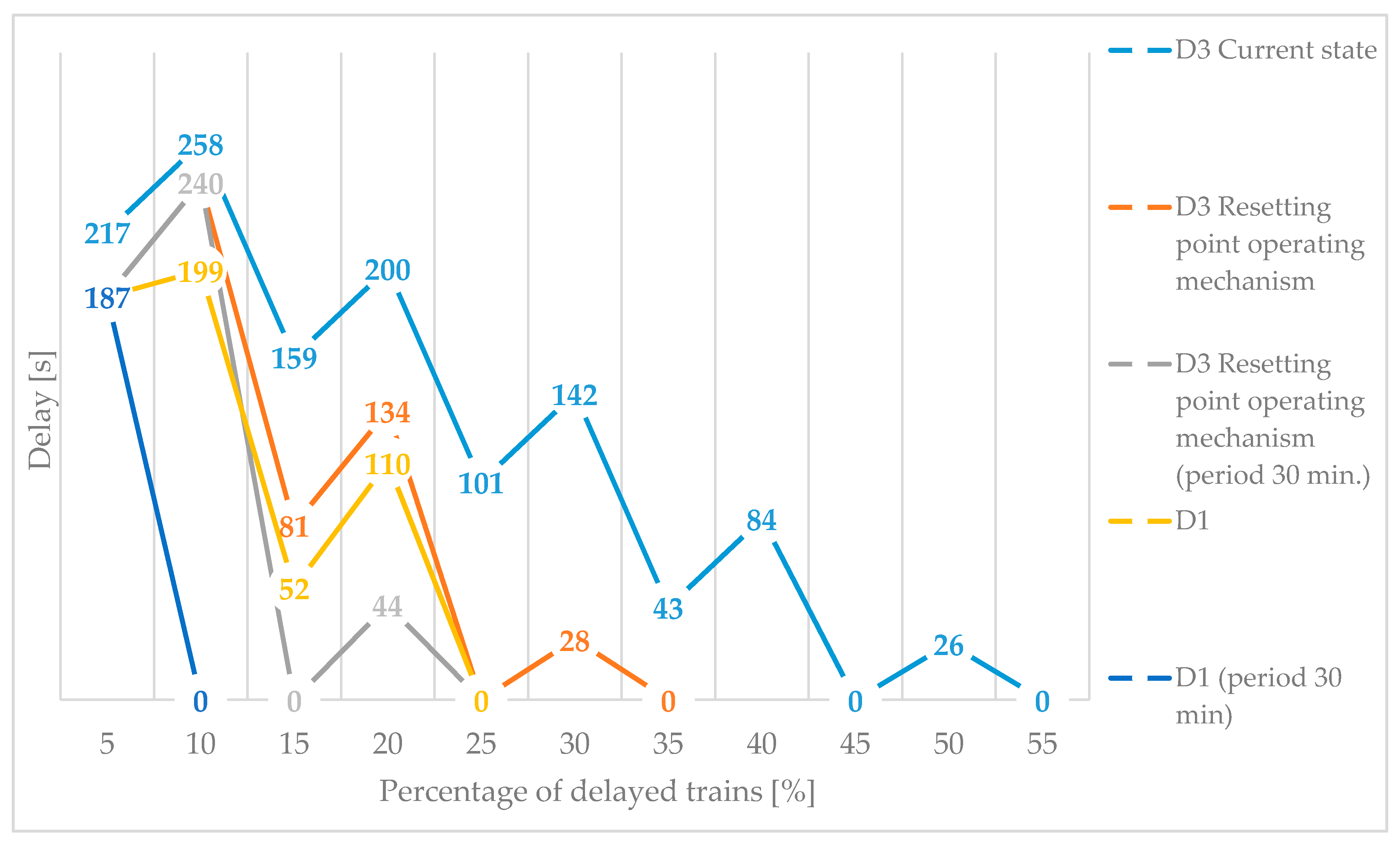
In the first stage of the simulation of the individual operational scenarios, an input delay of 300 s was considered for the first departing train from the Moravany station. Subsequently, the development of output delay was measured for individual trains up to the delay compensation point. Figure 6 shows the delay development in relation to the percentage of delayed trains. For objective comparison of the possible delays, 20 routes were created, i.e., 10 for each direction. We can see that the compensation point of the current state is after approx. 10 trains. If we add some technical equipment, such as resetting trailable points, the timetable can compensate for the delay after five trains (variant D3). A modern signaling system is the fastest (variant D1).
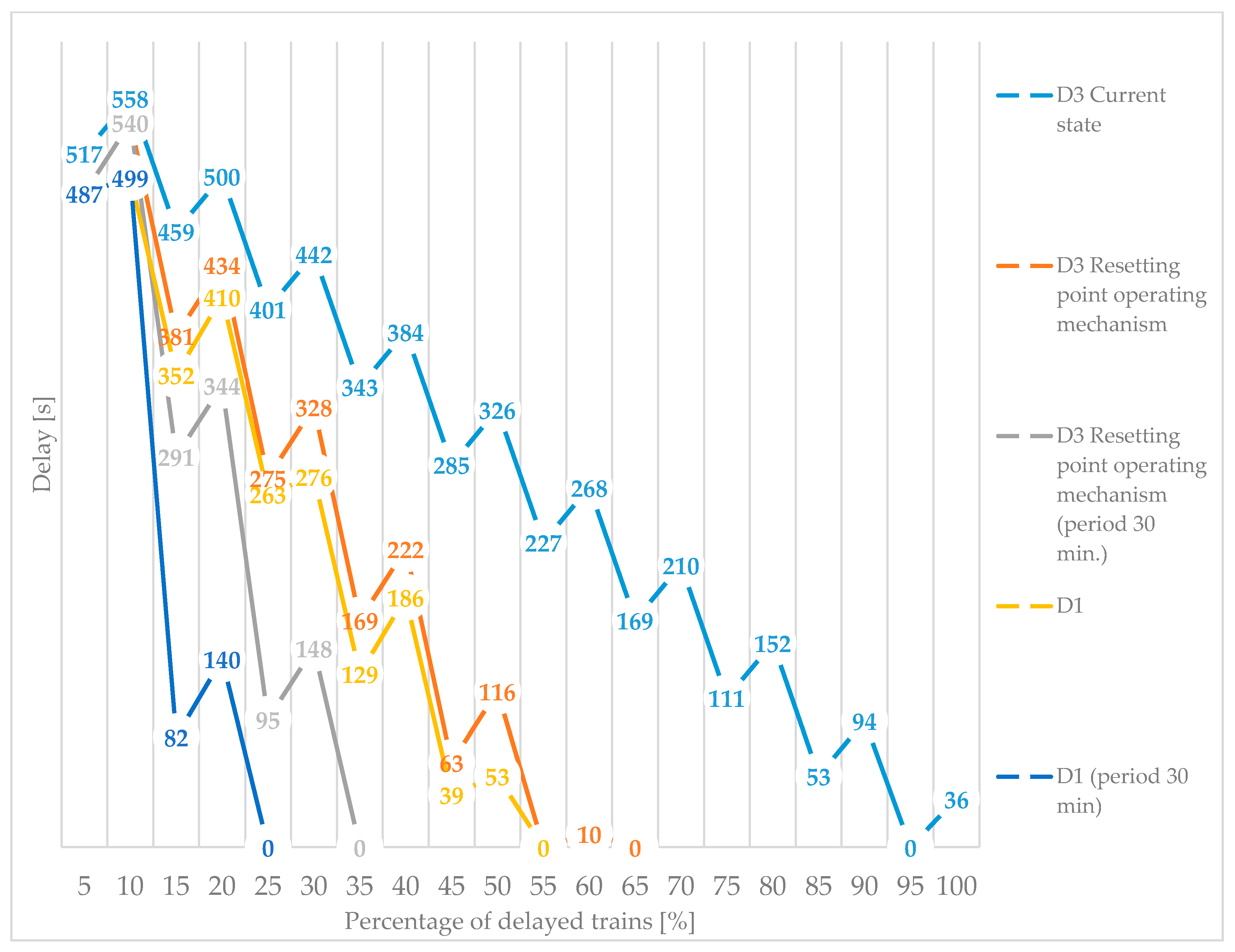
In the second stage, the input delay was increased to 600 s. The results are shown in Figure 6. As can be seen from the graph, the delay cannot be compensated in the calculation period (5 h) when simulating the maximum train diagram under existing conditions. The delay development reflects a trend already seen in Figure 7. Important is the fact that in all cases, there is a negative delay increment, and the delay is gradually compensated. The delay of 600 s shows similar results as in the previous simulation. We can see that even a minor investment in resetting trailable points has a huge effect on the delay compensation.
Another important step was to establish the delay compensation point Tx. This point is a specific temporal position in the train diagram created at which the input delay is compensated, and at the same time, from this point onwards, there are no more delays. To ensure the stability of the timetable, it is also important to follow the average delay increment (∆d) indicator, the values of which should lie within the optimum range established by the SŽDC SM 124 regulation. The average delay increment is calculated based on Equation 6. The disadvantage of this approach lies in the fact that it is primarily meant for railway lines with mixed traffic. To properly assess the quality and stability of a timetable using this method, the simulation would need to be replicated several dozen times.
where
- ∆d = average delay increment (min)
- dout = train output delay (min)
- din = train input delay (min)
- n = number of all trains included in the simulation (trains)
Table 4 shows the values of selected timetable (operational scenario) quality indicators. These include the percentage of delayed trains in the simulated time period D, the average delay increment ∆d and the delay compensation point Tx.
4.5. Evaluation of the Case Study and Proposed Changes
To select the acceptable variants, the following acceptance criteria were established based on the proposed timetable (operational scenario) quality indicators:
- Percentage of delayed trains D ≤ 30% with an input delay of 300 s, and D ≤ 35% with an input delay of 600 s;
- Peak period delay increment in accordance with the SŽDC SM 124 regulation must be in the optimum range, i.e., ∆d ≤ 30 s;
- Delay compensation point Tx ≤ 100 min.
Two acceptable variants were selected based on these criteria. The analysis of results showed that the highest quality is ensured by the operational concept, assuming equipping the line with a remotely controlled signaling system according to conventional rail regulations with a period of Tper = 30 min. This solution is included in variant D1 (period 30 min). This variant is also advantageous due to increasing traffic safety. Unfortunately, it could only be applied upon a complete reconstruction of the railway line, which would be very costly.
Another acceptable variant is the one considering the installation of resetting trailable points and a period of Tper = 30 min. This solution is included in variant D3 Resetting trailable points (period 30 min). This variant is mainly beneficial thanks to its simplicity and the possibility of rapid implementation without high investment costs. Its main advantage is the prevention of the undesirable extension of journey times and increasing the time loss due to the need for a member of the train crew to manually reset the points. For this reason, this variant seems to be the most advantageous one to be applied on the railway line under the current operational and technical conditions. Equipping the Holice station with resetting trailable points, with points in a priority position reset in every direction to another track, represents the simplest applicable system for the respective transport technology used.
5. Discussion
The aim of the paper was to invent a method for the simulation of traffic on lines with low traffic intensity and simplified interlocking, as well as a method of operation in the OpenTrack simulation software. This aim has been fulfilled. The conditions of the SŽ D3 regulation were arranged on the regional line Moravany—Holice—Borohrádek and the traffic was simulated and evaluated. This case study illustrates how such models can also be used for the assessment of changes in transport infrastructure. The assessment of the quality, throughput and stability of a timetable is a complex matter. On railway lines with low traffic intensity, there is almost no point in assessing throughput using conventional methods. Even though the results of these methods obtain accurate values, their significant use for these lines is not foreseen. The case study assessed different proposals using the following indicators: percentage of delayed trains, average delay increment, and delay compensation point. These indicators allow for the mutual comparison of the timetable variants proposed. There can be other limiting conditions added to these indicators to make the results even more accurate. What is also new is the conclusion about the relationship between the delay compensation and the signaling system. Small investments in infrastructure can bring much better values to the delay compensation.
In the future, based on the experience gained, and maintaining the close monitoring and assessing of the values obtained, it will be possible to establish recommended values as well, which will be applicable for assessing different traffic on different railway lines with low traffic intensity and simplified rail transport control. In this case, simulation is an ideal tool for assessing traffic, as it allows for the rapid and accurate evaluation of results. Another advantage is the fact that input parameters can be changed easily, which will be immediately reflected in the resulting journeys of the individual trains. Railway lines with low transport intensity remain an integral part of the transport systems of many countries. Quality traffic technologies and potential modifications leading to an improvement in traffic parameters and an increase in traffic quality can serve as a tool for economically viable traffic on these lines. Research in this area is therefore clearly desirable, and can potentially come up with new advantageous elements, which can help increase the attractiveness of these railway lines.
6. Conclusions
The main benefit of this article is its detailed functional simulation model carried out in SW OpenTrack. The article describes the possibility of the assessment of throughput on lines organized under simplified conditions. The analytical methods described in this article serve primarily as a guide for the preparation of the simulation model. By figuring out each part of the simulation model, we can find the decisive elements of a microscopic model of traffic organization. This principle is one possibility for how to solve that problem. The functionality of the model is proven by a case study applied together with an appropriate evaluation method. Due to the dispositions of the operation, whereby the degree of occupancy almost always exceeds the recommended values, a modified delay increment method is used for the calculation. This method helps us, within the simulation models, to verify the stability of the proposed maximum timetables, when we are coming close to the limits of the theoretical throughput of the track. In comparison with the available literature sources, the methodology used in this article brings a certain progressive element.
Author Contributions
P.N. and E.T. conceived and designed the simulation; J.Š. and J.G. analysed the data; P.N. and E.T. wrote the manuscript. All authors have read and agreed to the published version of the manuscript.
Funding
This article is published within the “Cooperation in Applied Research between the University of Pardubice and companies in the Field of Positioning, Detection and Simulation Technology for Transport Systems (PosiTrans)” project, registration No.: CZ.02.1.01/0.0/0.0/17_049/0008394.
Institutional Review Board Statement
Not applicable.
Informed Consent Statement
Not applicable.
Data Availability Statement
Not applicable.
Conflicts of Interest
The authors declare no conflict of interest. The funders had no role in the design of the study; in the collection, analyses, or interpretation of data; in the writing of the manuscript, or in the decision to publish the results.
References
- SŽDC (ČD). Služební Předpis Pro Stanovení Provozních Intervalů a Následného Mezidobí; D23; ČD: Praha, Czech Republic, 2002. [Google Scholar]
- SŽDC (ČD). Předpisy Pro Zjišťování Propustnosti Železničních Trait; D24; ČD: Praha, Czech Republic, 1966. [Google Scholar]
- International Union of Railways. UIC CODE, 2nd ed.; 406; International Union of Railways: Paris, France, 2013; Available online: https://tamannaei.iut.ac.ir/sites/tamannaei.iut.ac.ir/files//files_course/uic406_2013.pdf (accessed on 20 April 2020).
- Rotoli, F.; Navajas Cawood, E.; Soria, A. Capacity Assessment of Railway Infrastructure: Tools, Methodologies and Policy Relevance in the EU Context; EUR 27835 EN; Publications Office of the European Union: Brussels, Belgium, 2016. [Google Scholar] [CrossRef]
- International Union of Railways. Brakes—Braking Performance, 6th ed.; UIC CODE 544-1; International Union of Railways: Paris, France, 2020. [Google Scholar]
- SŽDC (ČD). Předpis pro Zjednodušené Řízení Drážní Dopravy; D3; ČD: Praha, Czech Republic, 2015. [Google Scholar]
- SŽDC SM 124. Zjišťování Kapacity Dráhy; SŽDC: Prague, Czech Republic, 2013; pp. 7–86. [Google Scholar]
- Taczanowski, J. A comparative study of local railway networks in Poland and the Czech Republic. Bull. Geogr. 2012, 18, 125–138. [Google Scholar] [CrossRef] [Green Version]
- Ljubaj, I.; Mikulčić, M.; Mlinarić, T.J. Possibility of Increasing the Railway Capacity of the R106 Regional Line by Using a Simulation Tool. Transp. Res. Procedia 2019, 44, 137–144. [Google Scholar] [CrossRef]
- Černá, L.; Ľupták, V.; Šulko, P.; Blaho, P. Capacity of main railway lines—Analysis of methodologies for its calculation. Naše More Int. J. Marit. Sci. Technol. 2018, 65. [Google Scholar] [CrossRef]
- Gašparík, J.; Stopka, O.; Pečený, L. Quality evaluation in regional passenger rail transport. Nase More 2015, 62, 114–118. [Google Scholar] [CrossRef]
- Dolinayova, A.; Danis, J.; Cerna, L. Regional railways transport-effectiveness of the regional railway line. In Sustainable Rail Transport: Proceedings of Rail Newcastle 2017; Springer: Cham, Switzerland, 2017; pp. 181–200. [Google Scholar]
- Wegelin, P.; von Arx, W. The impact of alternative governance forms of regional public rail transport on transaction costs. Case evidence from Germany and Switzerland. Res. Transp. Econ. 2016, 59, 133–142. [Google Scholar] [CrossRef]
- Zitrický, V.; Gašparík, J.; Pečený, L. The methodology of rating quality standards in the regional passenger transport. Transp. Probl. 2015, 10, 59–72. [Google Scholar] [CrossRef] [Green Version]
- Maulat, J.; Krauss, A. Using contrats d’axe to coordinate regional rail transport, stations and urban development: From concept to practice. Town Plan. Rev. 2014, 85, 287–311. [Google Scholar] [CrossRef]
- Lalinska, J.; Camaj, J.; Mašek, J.; Nedeliaková, E. Possibilities and solutions of compensation for delay of passenger trains and their economic impacts. In Proceedings of the 19th International Scientific Conference on Transport Means, Kaunas, Lithuania, 22–23 October 2015. [Google Scholar]
- Mašek, J.; Kendra, M.; Milinkovič, S.; Veskovič, S.; Bárta, D. Proposal and Application of Methodology of Revitalisation of Regional Railway Track in Slovakia and Serbia. Part 1: Theoretical Approach and Proposal of Methodology for Revitalisation of Regional Rail. Transp. Probl. 2015, 10, 85–95. [Google Scholar] [CrossRef] [Green Version]
- Dolinayová, A. Factors and determinants of modal split in passenger transport. Horiz. Railw. Transp. Sci. Pap. 2011, 1, 13–21. [Google Scholar]
- Liudvinavičius, L.; Dailydka, S.; Sładkowski, A. New Possibilities of Railway Traffic Control Systems. Transp. Probl. 2016, 11, 133–142. [Google Scholar] [CrossRef]
- Sipus, D.; Abramovic, B. The possibility of using public transport in rural area. Procedia Eng. 2017, 192, 788–793. [Google Scholar] [CrossRef]
- Dolinayova, A.; Cerna, L. Passenger and freight transport performances in the regional railway line and their impact to the state budget requirements—Case study in Slovakia. In Proceedings of the 23rd International Scientific Conference on Transport Means 2019, Palanga, Lithuania, 2–4 October 2019; Volume 2019, pp. 148–152. [Google Scholar]
- Mikulčić, M.; Petrović, M.; Ljubaj, I. Analysing the Railway Passenger Train Operation Using a Simulation Model. Horizons of Railway Transport. Strečno 2017, 9, 122–128. [Google Scholar]
- Abramović, B.; Pagasić Skrinjar, J.; Sipus, D. Analysis of railway infrastructure charges fees on the local passenger lines in Croatia. In Proceedings of the Third International Conference on The Traffic and Transport Engineering (ICTTE), Belgrade, Serbia, 24–25 November 2016; pp. 918–923. [Google Scholar]
- Janos, V.; Kriz, M. Pragmatic approach in regional rail transport planning. Sci. J. Sil. Univ. Technol. Ser. Transp. 2018, 100, 35–43. [Google Scholar]
- Fraszczyk, A.; Marinov, M. Sustainable Rail Transport: Proceedings of Rail Newcastle 2017; Springer: Cham, Switzerland, 2018; 307p, ISBN 9783319785448. [Google Scholar]
- Rybicka, I.; Stopka, O.; Ľupták, V.; Chovancová, M.; Droździel, P. Application of the methodology related to the emission standard to specific railway line in comparison with parallel road transport: A case study. MATEC Web Conf. 2018, 244. [Google Scholar] [CrossRef]
- Sładkowski, A.; Bizoń, K. The use of semi-automatic technique of finite elements mesh generation for solutions of some railway transport problems. J. Mech. Solid Bodies 2017, 23. [Google Scholar] [CrossRef] [Green Version]
- Yong, C.; Ullrich, M.; Weiting, Z. Calibration of disturbance parameters in railway operational simulation based on reinforcement learning. J. Rail Transp. Plan. Manag. 2016, 6, 1–12. [Google Scholar] [CrossRef]
- Bulíček, J.; Bažant, M. Selection of railway line segments that allow occupation by more trains based on simulation. In Proceedings of the 32nd European Modeling and Simulation Symposium, Athens, Greece, 16–18 September 2020. [Google Scholar] [CrossRef]
- Bešinović, N.; Quaglietta, E.; Goverde, R.M.P. A simulation-based optimization approach for the calibration of dynamic train speed profiles. J. Rail Transp. Plan. Manag. 2013, 3, 126–136. [Google Scholar] [CrossRef] [Green Version]
- Burdett, R.L. Optimisation models for expanding a railway’s theoretical capacity. Eur. J. Oper. Res. 2016, 251, 783–797. [Google Scholar] [CrossRef]
- Straka, M.; Saderova, J.; Bindzar, P.; Malkus, T.; Lis, M. Computer simulation as a means of efficiency of transport processes of raw materials in relation to a cargo rail terminal: A case study. ACTA Montan. SLOVACA 2019, 24, 307–317. [Google Scholar]
- De Martinis, V.; Corman, F. Online microscopic calibration of train motion models Towards the era of customized control solutions. In Proceedings of the 8th International Conference on Railway Operations Modelling and Analysis—Rail Norrköping 2019, Norrköping, Sweden, 17–20 June 2019; pp. 917–932. [Google Scholar] [CrossRef]
- Marinov, M.; Viegas, J.A. Mesoscopic simulation modelling methodology for analyzing and evaluating freight train operations in a rail network. Simul. Model. Pract. Theory 2011, 19, 516–539. [Google Scholar] [CrossRef]
- SŽDC SM 104. Provozní Intervaly a Následná Mezidobí; SŽDC: Prague, Czech Republic, 2019; pp. 23–90. [Google Scholar]
Figure 1.
Schematic representation of the different stages of simulation model preparation. Source: Authors, based on Ref. [29].
Figure 1.
Schematic representation of the different stages of simulation model preparation. Source: Authors, based on Ref. [29].

Figure 2.
Diagram of route creation. Source: Authors.

| A1 | Exit signal from third station track |
| A2 | Exit signal from first station track |
| A3 | Home signal |
| A4 | Remotely controlled point |
| A–B | Interstation section between stations A and B |
| B1 | Fictitious stopping point before outer point (fictitious operating point) |
| B2 | Locally controlled point |
| B3 | Fictitious exit signal from first station track |
| B4 | Fictitious exit signal from third station track |
| B5 | Fictitious exit signal from third station track |
| B6 | Fictitious exit signal from first station track |
| B7 | Locally controlled point |
| B8 | Fictitious stopping point before outer point (fictitious operating point) |
| B–C | Interstation section between stations B and C |
| C1 | Home signal |
| C2 | Remotely controlled point |
| C3 | Starting signal from third station track |
| C4 | Starting signal from first station track |
Figure 3.
Flowchart of the modified method of model preparation. Source: Authors.

Figure 4.
Holice station model in an OpenTrack worksheet. Source: Authors, based on SW OpenTrack.

Figure 5.
Tachograph for freight (top) and passenger (bottom) trains in the section Moravany–Borohrádek. Source: Authors, based on SW OpenTrack.
Figure 5.
Tachograph for freight (top) and passenger (bottom) trains in the section Moravany–Borohrádek. Source: Authors, based on SW OpenTrack.

Figure 6.
Graph representing the delay development with an input delay of 5 min. Source: Authors, based on SW OpenTrack.
Figure 6.
Graph representing the delay development with an input delay of 5 min. Source: Authors, based on SW OpenTrack.

Figure 7.
Graph representing the delay development with an input delay of 10 min. Source: Authors, based on SW OpenTrack.
Figure 7.
Graph representing the delay development with an input delay of 10 min. Source: Authors, based on SW OpenTrack.


Table 1.
Parameters of reference trainsets. Source: Authors, based on OpenTrack.
| Reference Trainset | Maximum Speed (km/h) | Weight (t) | Length (m) | Maximum Tractive Force (kN) | Maximum Power (kW) | Maximum Deceleration (m.s−2) |
|---|---|---|---|---|---|---|
| ČD 810 | 80 | 24 | 14 | 29 | 155 | −0.6 |
| ČD 814 | 80 | 54.8 | 28.5 | 54 | 242 | −0.6 |
| ČDC 742 + trainset | 80 | 500 | 200 | 192 | 883 | −0.6 |
Table 2.
Comparison of journey times. Source: Authors, based on SW OpenTrack.
| Moravany–Holice | Holice–Moravany | Holice–Borohrádek | Borohrádek–Holice | |||||||||
|---|---|---|---|---|---|---|---|---|---|---|---|---|
| Trainset | GVD | OT | ∆ | GVD | OT | ∆ | GVD | OT | ∆ | GVD | OT | ∆ |
| ČD 814 | 720 | 698 | 22 | 720 | 712 | 8 | 720 | 674 | 46 | 660 | 644 | 16 |
| ČD 814 (p) | 870 | 865 | 5 | 900 | 879 | 21 | 870 | 857 | 13 | 840 | 812 | 28 |
| ČDC 742 | 900 | 703 | 197 | 900 | 673 | 227 | 960 | 912 | 48 | 900 | 696 | 204 |
GVD—journey time taken from the traffic diagram created (s); OT—actual journey time established through simulation (s); ∆—difference between both journey times (s); ČD 814 (p)—journey times for ČD 814 extended by the time needed for point resetting.
Table 3.
Comparison of journey times. All values in seconds. Source: Authors, based on SW OpenTrack.
Table 3.
Comparison of journey times. All values in seconds. Source: Authors, based on SW OpenTrack.
| Operating Interval | M (H) | H (M) | H (B) | B (H) |
|---|---|---|---|---|
| Ivv (of successive arrivals) | 810 (960) | 840 (990) | 810 (960) | 810 (960) |
| Iov (of departure and arrival) | 1530 (1680) | 1560 (1710) | 1470 (1620) | 1470 (1620) |
| Ivo (of arrival and departure) | 60 | 150 | 150 | 120 |
| Ioo (of successive departures) | 840 (990) | 810 (960) | 810 (960) | 810 (960) |
| INJ (of subsequent journeys) | 840 (990) | 810 (960) | 810 (960) | 810 (960) |
Ivv—operating interval of successive arrivals; Iov—operating interval of departure and arrival; Ivo—operating interval of arrival and departure; Ioo—operating interval of successive departures; INJ—operating interval of subsequent journeys; M (H)—Moravany station (direction Holice); H (M)—Holice station (direction Moravany); H (B)—Holice station (direction Borohrádek); B (H)—Borohrádek station (direction Holice); The values in brackets stand for the interval value in case the second train stops in Holice for point resetting (extension of the journey time by 150 s).
Table 4.
Selected timetable quality indicators. Source: Authors, based on SW OpenTrack.
| Operational Scenario | Input Delay of 300 s | Input Delay of 600 s | ||||
|---|---|---|---|---|---|---|
| D (%) | ∆d (min) | Tx (min) | D (%) | ∆d (min) | Tx (min) | |
| D3 Current state | 55 | −0.28 | 186 | 100 | −0.49 | >300 |
| D3 Resetting trailable points | 30 | −0.04 | 80.5 | 60 | −0.08 | 161 |
| D3 Resetting trailable points (period 30 min.) | 25 | 0.16 | 55 | 35 | 0.16 | 94.5 |
| D1 | 30 | −0.20 | 61 | 60 | −0.40 | 70.5 |
| D1 (period 30 min.) | 10 | 0.07 | 30 | 20 | 0.13 | 60 |
Publisher’s Note: MDPI stays neutral with regard to jurisdictional claims in published maps and institutional affiliations. |
© 2021 by the authors. Licensee MDPI, Basel, Switzerland. This article is an open access article distributed under the terms and conditions of the Creative Commons Attribution (CC BY) license (http://creativecommons.org/licenses/by/4.0/).
Share and Cite
MDPI and ACS Style
Široký, J.; Nachtigall, P.; Tischer, E.; Gašparík, J. Simulation of Railway Lines with a Simplified Interlocking System. Sustainability 2021, 13, 1394. https://0-doi-org.brum.beds.ac.uk/10.3390/su13031394
AMA Style
Široký J, Nachtigall P, Tischer E, Gašparík J. Simulation of Railway Lines with a Simplified Interlocking System. Sustainability. 2021; 13(3):1394. https://0-doi-org.brum.beds.ac.uk/10.3390/su13031394
Chicago/Turabian StyleŠiroký, Jaromír, Petr Nachtigall, Erik Tischer, and Jozef Gašparík. 2021. "Simulation of Railway Lines with a Simplified Interlocking System" Sustainability 13, no. 3: 1394. https://0-doi-org.brum.beds.ac.uk/10.3390/su13031394
Note that from the first issue of 2016, this journal uses article numbers instead of page numbers. See further details here.