Comprehensive Measurement and Regional Imbalance of China’s Green Development Performance


1
Research Center of the Central China for Economic and Social Development, Nanchang University, Nanchang 330031, China
2
School of Economics and Management, Nanchang University, Nanchang 330031, China
*
Author to whom correspondence should be addressed.
Sustainability 2021, 13(3), 1409; https://0-doi-org.brum.beds.ac.uk/10.3390/su13031409
Submission received: 8 January 2021
/
Revised: 24 January 2021
/
Accepted: 25 January 2021
/
Published: 29 January 2021
(This article belongs to the Section Economic and Business Aspects of Sustainability)
Abstract
:This study adopted the two-stage super-efficiency network slack-based model (SBM) to measure the green development performance index (GDPI) of 30 provinces in China. The Dagum Gini coefficient decomposition was used to analyze the regional differences and their sources in China’s green development performance. The results are as follows: first, the green development performance showed a declining trend from 1997 to 2017. The improvement of environmental governance efficiency was the key to achieving green development progress. The green development levels of coastal areas were significantly higher than those of inland provinces. Second, the regional imbalance in China’s green development performance was gradually worsening. The inter-regional differences were the primary source of the overall differences. The intra-regional difference of green development within the northwest was the largest. Third, among the eight regions, only the southwest region had σ convergence in green development performance; in addition, absolute β convergence and conditional β convergence were divergent, thereby confirming the regional imbalance of the widening regional differences in China’s green development performance. This study aimed to provide a scientific basis and effective reference for further advancing China’s regional coordinated development strategy.
1. Introduction
Harmony between economic growth, environmental protection, and sustainable development after industrialization are global concerns. The green development model emphasizes the improvement of resource use efficiency and environmental damage avoidance. Moreover, the improvement of green development performance is in line with the sustainable development goals (SDGs). Green development performance integrates two constraints in economic development. It reduces resource consumption and improves environmental quality [1]. The higher the value, the higher the level of green development.
China exhibited an economic growth miracle as its GDP grew by almost 230 times from 1978 to 2019. However, its economy still follows an extensive development model driven by resources and energy [2], resulting in severe ecological pressure on economic and social development. Urbanization and industrialization have intensified the effects of such an economic model [3]. China ranked 120th in the Global Environmental Performance Index Report (2020) released by Yale University, indicating that its environmental performance is still far behind that of the rest of the world. As the world’s largest developing country and energy user [4], assessing China’s green development status can help policymakers formulate policies to improve its green development. At the same time, other countries may take this resource-saving, environmentally friendly green development path as a reference.
Research on green development performance has received extensive attention since the 1990s. Kortelainen [5] conducted a comparative analysis of 20 European Union member states’ environmental performance from 1990 to 2003 using data envelopment analysis (DEA). Jena [6] used the Luenberger productivity index to assess the environmental efficiency of 19 states in India from 1991 to 2003. The result showed that India’s rapid economic growth poses severe environmental problems. Chinese studies on green development performance are also gradually increasing. Some scholars have quantitatively analyzed China’s three major regions’ green development levels, using the east, central, and west regions as research units [7]. Still, this method can neither accurately reflect China’s regional green development performance nor reveal the spatial imbalance of China’s regional green development performance in more detail [8]. Compared with China’s traditional division of the three regions, the eight economic regions divided by the State Council’s Development Research Center based on nine principles are more specific. China’s eight economic regions have significant regional differences in many respects [9,10,11]. Using these eight major economic regions as research units to study China’s green development performance and revealing in detail the spatial imbalance in the country’s regional green development performance, the analysis is theoretically richer and of more practical significance for future policy formulation.
Research on green development mainly focuses on efficiency measurement [12,13], exploration of influencing factors [14,15], and testing of convergence mechanisms [16,17]. In terms of the measurement of green development performance, most scholars mainly use efficiency measurement methods such as the stochastic frontier approach [18], data envelopment analysis (DEA) [19,20], and total factor productivity (TFP) [21] to measure the green development performance of specific industries, city groups, and three or four major regions in China. Data envelopment analysis (DEA), proposed by Charnes [22], is widely used to measure efficiency because it eliminates the need to set a production function and avoids a subjective assignment of input and output indicators. Traditional DEA models, such as CCR and BCC models, have radial or angular defects, leading to low measure efficiency and accuracy. Tone [23] proposed a slack-based model (SBM) on the basis of slack variables. The SBM model solves radial and angular problems. However, it cannot sort effective decision units when the decision-making unit has an efficiency value of 1. Therefore, Tone [24] proposed the super-efficiency SBM model, which is a total revamp of the simple SBM model. Subsequent studies have extensively used the super-efficiency SBM model. The super-efficiency SBM model is one of the most common models used by scholars to study green development performance. Loikkanen and Susiluoto [25] used a DEA model to assess the private sector’s economic efficiency in 83 regions of Finland from 1988 to 1999. Zhao et al. [15] used the super-efficiency SBM model, considering undesirable outputs, to measure and analyze eight economic regions’ green economic efficiency in China. Moreover, they used the spatial Durbin model considering the geographical distance to analyze the influencing factors affecting green economic efficiency. Yang et al. [12] used the super-efficiency DEA model to measure the green sustainable development efficiency and TFP of 31 provinces in China. The measurement of green development performance must consider economic growth and environmental governance [1]. The above studies treat the green development process as achieving economic growth while causing environmental pollution; however, such a process ignores the positive role of environmental governance on green development. Given this factor, the present study innovatively applied the network DEA model proposed by Fare (1991) [26] and Fare and Grosskopf (1996) [27] to construct a comprehensive evaluation index system for green development in economic production and environmental governance. It conducted a comparative analysis of China’s eight major economic regions’ green development levels to put forward feasible suggestions for improving the green development levels of each region.
Significant regional differences exist in China’s green development performance at the provincial [28] and regional levels [29]. Scholars use the intuitive comparison of efficiency [15,20] and Thiel index [30] to study regional green development performance differences. Intuitive comparisons of efficiency do not reveal the sources of regional differences. Although Theil index solves the problem of revealing the sources of regional differences, it is sensitive to the probability distribution of the data [31]. The Gini coefficient by the subgroup decomposition method proposed by Dagum [32] in 1997 overcomes these problems and more effectively identifies the sources of regional differences. The Dagum Gini coefficient decomposition is currently widely applied to the regional difference in PM2.5 concentration [33], agricultural eco-efficiency [34], urban land-use efficiency [35], and carbon emission [36]. However, such studies are rare in terms of differences in green development performance, especially when the eight economic regions are used as research units. To well promote coordinated regional development and reduce regional disparities in green development levels, identifying the sources of regional disparities using the Dagum Gini coefficient decomposition is necessary.
The current study aims to construct an evaluation index system of green development performance to examine China’s green development performance status. We find differences in green development performance in eight economic regions, which prove the unbalanced regional green development pattern in the country. We use Dagum’s decomposition of the Gini coefficient to answer whether the gap between the regional green development levels of China’s eight economic regions is widening or narrowing. We also test whether inter-regional differences or intra-regional differences are responsible for this result. The results can help policymakers formulate targeted policies to narrow the regional green development gap and promote regional green and coordinated development.
Compared with previous studies, the marginal contributions of this research are in the following two aspects. First is the innovation of the research scale. Using the eight economic regions as research units, we can realistically reflect the changing characteristics of each economic region’s green development performance and accurately reveal the uneven pattern of regional development, laying a solid foundation for policies to improve green development levels and promote coordinated regional development. Second is the innovation of research content. Existing studies mostly focus on analyzing regional imbalance laws, and the deconstruction of regional differences in the eight major economic regions is insufficient. This study measures the green development performance index (GDPI) of China’s 30 provinces (city and autonomous regions), considering economic production and environmental governance. It identifies the sources of regional differences by using the Dagum Gini coefficient decomposition, which provides essential references for promoting the coordinated development of China’s eight major economic regions and improving regional imbalances in the new period.
2. Materials and Methods
2.1. Materials
2.1.1. Division of Economic Regions
This study comprehensively measures the GDPI of 30 provinces in China and explores its regional differences. To identify the effects of inter-regional and intra-regional differences further on the overall regional differences, we use eight economic regions by the Development Research Center of the State Council of China as the study units (Table 1).
2.1.2. Analytical Framework of Green Development Performance
Following previous studies, this research decomposes the whole process of green development into economic production and environmental governance, both of which are measured using the two-stage super-efficiency network SBM model. Figure 1 decomposes the green development performance transformation system into two transformation subsystems: economic production and environmental governance efficiency. It comprehensively measures the green development performance of 30 provinces in China from 1997 to 2017.
In the first stage, the inputs of energy consumption, capital, water resources, labor, and land resources bring economic growth and environmental pollution through the transformation subsystem of economic production efficiency (GPE). In the intermediate link of the first and second stages, the environmental governance investment as the intermediate input obtains the environmental governance effect through the environmental governance efficiency (GEE) transformation subsystem.
2.1.3. Index Selection and Data Source
On the basis of the two-stage network super-efficiency SBM model, the evaluation index system of China’s GDPI is constructed (Table 2). According to existing research, this study selects five elements of capital, labor, energy, water resources, and land resources as input variables in the stage of economic production. Existing studies commonly use GDP as an expected output. In this study, the GDP of 30 provinces in China from 1997 to 2017 is selected as the expected output and is converted into a constant price on the basis of the year 2000. Considering data integrity and accessibility, this study sets wastewater, SO2, and industrial solid waste discharge as the undesirable outputs of economic production and the input variables in environmental governance. In the stage of environmental governance, the investment in the treatment of environmental pollution is added as an intermediate variable.
In the stage of economic production, capital investment is characterized by capital stock. Most existing literature uses a perpetual inventory method to calculate capital stock and formula to calculate capital stock. The base period capital stock uses the formula , , and respectively represent i province’s capital stock in t period, the total investment in fixed assets, and the capital depreciation rate. is the geometric average growth rate of total investment in fixed assets in i region. Before estimating the capital stock, society’s fixed asset investment has converted to a constant price on the basis of the year 2000. Energy consumption, coal, and other eight kinds of energy (The eight energy sources are coal, coke, kerosene, gasoline, crude oil, diesel oil, fuel oil, and natural gas. The corresponding conversion standard coal coefficient comes from China Energy Statistics Yearbook 2018) consumption are converted into standard coal to represent energy input.
The total number of employed persons in each province comes from China Provincial Statistical Yearbook. The total investment in fixed assets, per capita water consumption data, regional GDP, and area of built districts of each province come from China Statistical Yearbook (1998–2018) [37]. Data on the consumption of eight kinds of energy come from China Energy Statistical Yearbook (1998–2018) [38]. The data of wastewater, SO2 emissions, industrial solid waste, investment in the treatment of environmental pollution, wastewater and waste gas treatment facilities, treatment of industrial wastewater, and comprehensive utilization of solid waste are all from China Environmental Statistics Yearbook (1998–2018) [39].
We calculate the green development performance of 30 Chinese provinces by using MAXDEA software. Then, we employ Stata 15.0 software to determine the σ convergence and β convergence results for the eight economic regions in China.
2.2. Methods
2.2.1. Two-Stage Super-Efficiency Network SBM Model
To comprehensively investigate the green development level of each province in China, we used the two-stage super-efficiency network SBM. represents green development performance. The formula for calculating the green development performance can be expressed as Equation (1).
In Equation (1), mk and vk respectively denote the numbers of inputs and outputs of stage k, and denotes the number of intermediate indicators. (k, h) denotes the connection from stage k to stage h. x represents the input, y represents the output, z represents the intermediate output, denotes the model weight for stage k, and wk denotes the weight for stage k. denotes the input indicators’ slack variables. and represent the slack variables for the desired and undesiredutputs, respectively.
2.2.2. Dagum Gini Coefficient Decomposition
Gini coefficient is an important index to measure the degree of regional imbalance. The Dagum Gini coefficient decomposition proposed by Dagum in 1997 can measure the degree of regional imbalance and find regional difference sources. According to the Dagum Gini coefficient decomposition, the overall Gini coefficient (G) is decomposed into three parts: contribution of intra-regional difference (), contribution of inter-regional difference (), and contribution of super-variable intensity (). The components satisfy Formula (5): . G is calculated using Formula (2), revealing differences in green development performance in all provinces.
where represents the GDPI of j(r) provinces in the i(m) economic region. n, k, and . are the number of provinces, the number of regions, and the number of provinces in the i(m) economic region, respectively. μ is the average GDPI of each economic region and is sorted according to the average GDPI of the region.
Formulas (3) and (4) represent the Gini coefficient of i economic region and the inter-regional Gini coefficients of i and m economic regions, respectively. In Formula (9), represents the relative influence of GDPI between i and m economic regions. in Formula (10) represents the difference in GDPI between economic regions, that is, all is the mathematical expectation of the sum of the sample values in i and m economic regions; is the mathematical expectation of the sum of the sample values of all in i and m economic regions, and Fi (Fm) is the cumulative density distribution function of the i(m) economic region.
2.2.3. Analysis of Convergence
To investigate the levels of GDPI changes overtime in eight economic regions, σ convergence, and β convergence methods were used. The coefficient of variation [40,41] is usually used to measure the σ coefficient and use it to determine whether σ convergence exists or not. The model is as follows:
where σt denotes the coefficient of variation, ni is the number of regions, GDPIit represents the green development performance of region i in year t, and ()¯ refers to the average value of green development performance of all provinces in t year.
β convergence is divided into absolute β convergence and conditional β convergence. Absolute β convergence means that the green development performance of each economic regions will gradually converge at the same level over time. Regions with lower green development levels have higher growth rates compared with economic regions with higher green development levels. Conditional β convergence means that the green development performance of each economic region will converge at their steady state level under the action of a series of influencing factors. Referencing the studies of Lu and Xu [41], Cui et al. [16], and Xu et al. [17], this research sets the absolute β convergence model and conditional β model of GDPI growth on the basis of panel data as follows:
Equations (13) and (14) are the absolute β convergence model and the conditional β convergence model, respectively. ln(GDPIi,t+1/GDPIi,t) indicates the growth rate of the green development performance of regional i from t period to t+1 period. lnGDPIi,t represents the logarithm of the green development performance of region i in period t. μi is individual fixed effect, and vt is the time fixed effect. Using robust standard errors clustered at the provincial level, X denotes the control variable. In this study, technology level (tec), industrial structure (ind), energy structure (est), and openness (open) are selected as control variables.
In Equation (13), if β is significantly negative, then it indicates that the absolute β convergence exists in China’s green development performance. Regions with low green development performance levels have a catch-up effect on regions with high green development performance levels that regional differences in green development performance are gradually narrowing. The opposite is divergence, and regional differences in green development performance are widening. In the regression process, each control variable is processed in logarithm, and a two-way fixed-effect model, which simultaneously controls individual fixed effects and time fixed effects, is adopted.
3. Results
3.1. Green Development Performance and the Efficiency of Sub-Links
3.1.1. Comprehensive Evaluation of Green Development Performance
According to the calculation, the green development performance in China varies greatly between provinces. Figure 2 reveals the difference in the average green development performance (GDPI) of 30 provinces (city and autonomous regions) in China from 1997 to 2017. The map shows that the GDPI of the 30 provinces of China presents the characteristics of high in eastern and low in western, and the GDPI of both sides of China is quite different from that of Hu Line as the boundary. According to the GDPI of provinces, when environmental pollution and environmental governance factors are included in the evaluation index system of green development, the average annual GDPI of more than half of provinces is less than 1. From the green development level of each economic region, the GDPI from high to low are followed by the southern coast (1.1989), the northern coast (1.1973), the eastern coast (1.1378), the middle Yangtze River (0.9007), the middle Yellow River (0.8750), the southwest (0.7890), the northeast (0.7626), and the northwest (0.4857). By comparing green development performance between provinces and between economic regions, we find that the areas with high green development performance mostly concentrate in economically developed coast areas where the energy-saving and emission reduction standards are stringent, and the pollution treatment technology is advanced. However, the middle Yangtze River and the middle Yellow River, the southwest, and the northeast areas pay too much attention to the economic growth under the policies of the rise of central China, the significant development of the western part, and the revitalization of the northeast, respectively. They ignore the negative impact on the environment. Meanwhile, under the combined action of the backward economy and bad ecological environment, the performance value of green development in northwest China is at the end of the eight economic regions.
3.1.2. Comparative Analysis of Green Development Performance and Sub-Link Efficiency
Figure 3 illustrates that GDPI lies between economic production efficiency and environmental governance efficiency that shows a downward trend from 1997 to 2017, and the direction of the three lines is the same. From 1997 to 2017, the contribution of economic production efficiency to GDPI was always higher than that of environmental governance efficiency to GDPI. China’s traditional extensive mode of economic development depends too much on the input of resources. Although this mode keeps the economy growing at high speed, the damage to the environment makes China’s environment governance efficiency lower than the economic production efficiency from 1997 to 2017. From 1997 to 2010, the contribution of environmental governance efficiency to green development was relatively stable. After 2010, the contribution of environmental governance efficiency to green development performance increased year by year. However, environmental governance efficiency is still lower than economic production efficiency. At the current stage, the improvement of environmental governance efficiency is still the key to enhance the level of green development in China. We also conduct Pearson correlation tests for GDPI, GPE, and GEE (Table 3).
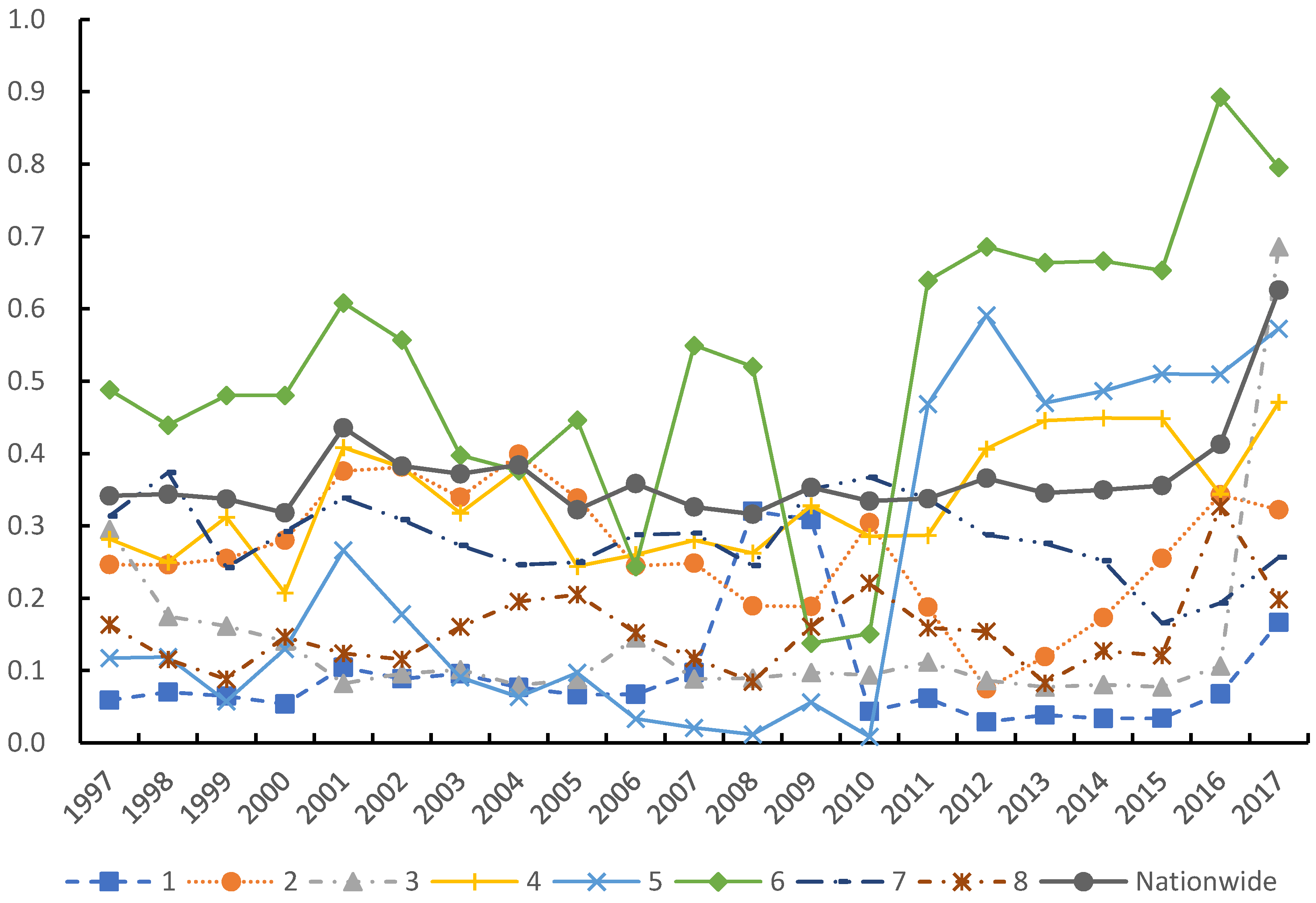
The GDPI of the eight economic regions is analyzed. The GDPI of the eight economic regions has an average annual score of 0.9026 in 21 years, and the overall DEA is inefficient. Figure 4 reflects the evolution trend of green development performance in China’s eight economic regions from 1997 to 2017. The GDPIs of the southern coast, northern coast, and eastern coast were located at the top of the eight economic regions in 1997–2009, 2010–2016, and 2017, respectively. The GDPI of the northwest region was at the end of the eight economic regions, except in 2014 and 2015. The GDPI of the southern coast region showed a continuous downward trend from 1997 to 2017 with a significant decrease in 2011. Fujian and Guangdong provinces’ GDPIs in southern coastal areas have always been effective. Hainan province’s GDPI showed a significant decline after 2011, which is the main reason the southern coastal areas’ GDPI exhibited a downward trend after 2011. The continuous increase of industrial solid waste in Hainan Province after 2011 and its comprehensive utilization rate are far lower than the average levels in other provinces, which is an important reason for the inefficiency and continuous decline of green development performance in Hainan after 2011. The GDPI of northern coastal region is relatively stable and is in the highest position of the eight economic regions. From 1997 to 2017, the eastern coast’s GDPI showed an upward trend and was the average value above 1. The GDPI of Shanghai directly affects the overall efficiency of green development in the eastern coastal region. In 2017, Shanghai significantly reduced pollutant emissions by developing green low-carbon clean energy, promoting clean production by industrial enterprises in the region, and developing green transportation. These measures made the GDPI of eastern coastal region in 2017 appear as a warp tail phenomenon. The middle Yangtze River and the middle Yellow River’s GDPIs showed fluctuating downward trends. The GDPI of northeast China exhibited a downward trend before 2009 and an upward trend after 2009. The southwest region’s GDPI is bounded by the year 2008, with an upward trend before 2008 and a downward trend after 2008. Northwest China’s GDPI exhibited a downward trend from 1997 to 2003 and a fluctuating upward trend from 2004 to 2017. The backwardness of water conservancy and telecommunication infrastructures in the northwest economic region hinders economic development. Moreover, large water conservancy, telecommunication, and industrial projects aggravate soil erosion and land desertification in the region. This contradiction creates great difficulties for local governments to carry out environmental governance. Especially after 1999, severe environmental problems emerged in the process of infrastructure construction and foreign investment attraction.
From 1997 to 2017, the southern coastal region and the northwest region recorded the highest and lowest mean values of GDPI. The decline of green development performance in Hainan Province after 2011 is the main reason for the decline of green development performance in southern coastal areas after 2011. The rise of green development performance in Shanghai in 2017 is the reason for the significant improvement of green development performance in eastern coastal areas in 2017. The green development performance of northern coast, eastern coast, and northwest regions improved from 1997 to 2017, whereas that of the remaining economic regions declined to various degrees (Figure 5). Green development performance becomes progressively smaller from east to west, and significant regional disparities are observed in the green development levels.
To analyze economic productivity and environmental governance efficiency, the two-stage super-efficiency network SBM model is applied for deconstructing green development performance into economic production efficiency and environmental governance efficiency. Figure 6 illustrates that Beijing, Hebei, Tianjin, Shanghai, Zhejiang, Jiangsu, and Fujian Provinces (cities) have performed well in the two sub-links of green development, basically realizing the coordinated development of economy and environment. Their advantages in economic production and environmental governance should be further consolidated in future development and provide a reference for other regions’ development. Provinces such as Shandong, Guangdong, and Hainan have performed well in economic production in green development. Environmental governance efficiency is a constraint to improve green development performance, which should further increase environmental governance, implement energy conservation and emission reduction targets. The provinces of Anhui, Hunan, and Yunnan have high environmental governance efficiency. Inadequate economic growth is a significant constraint on their green development performance. Regions represented by fragile natural environments such as Ningxia, Gansu, and Qinghai have relatively low economic production efficiency and environmental governance efficiency, both of which do not meet green development requirements. Therefore, efforts should be made to increase environmental governance investment while working for economic growth. The path in line with its green development must be explored, whereas economic and environment coordinated development should be promoted.
Figure 7 presents that regions with high economic production efficiency in China are distributed in the northern coast, eastern coast, and the southern coast. Environment governance efficiency shows a decreasing feature extending from the southeast to the northwest.
From the above analysis, a regional imbalance is observed in the green development levels in China. Reducing regional differences in the new period is of great practical significance for constructing the regional cooperative development mechanism in the country. The next part of this paper measures and analyzes the regional differences of green development performance between regions.
3.2. Analysis of Regional Differences in Green Development Performance
3.2.1. Overall Difference
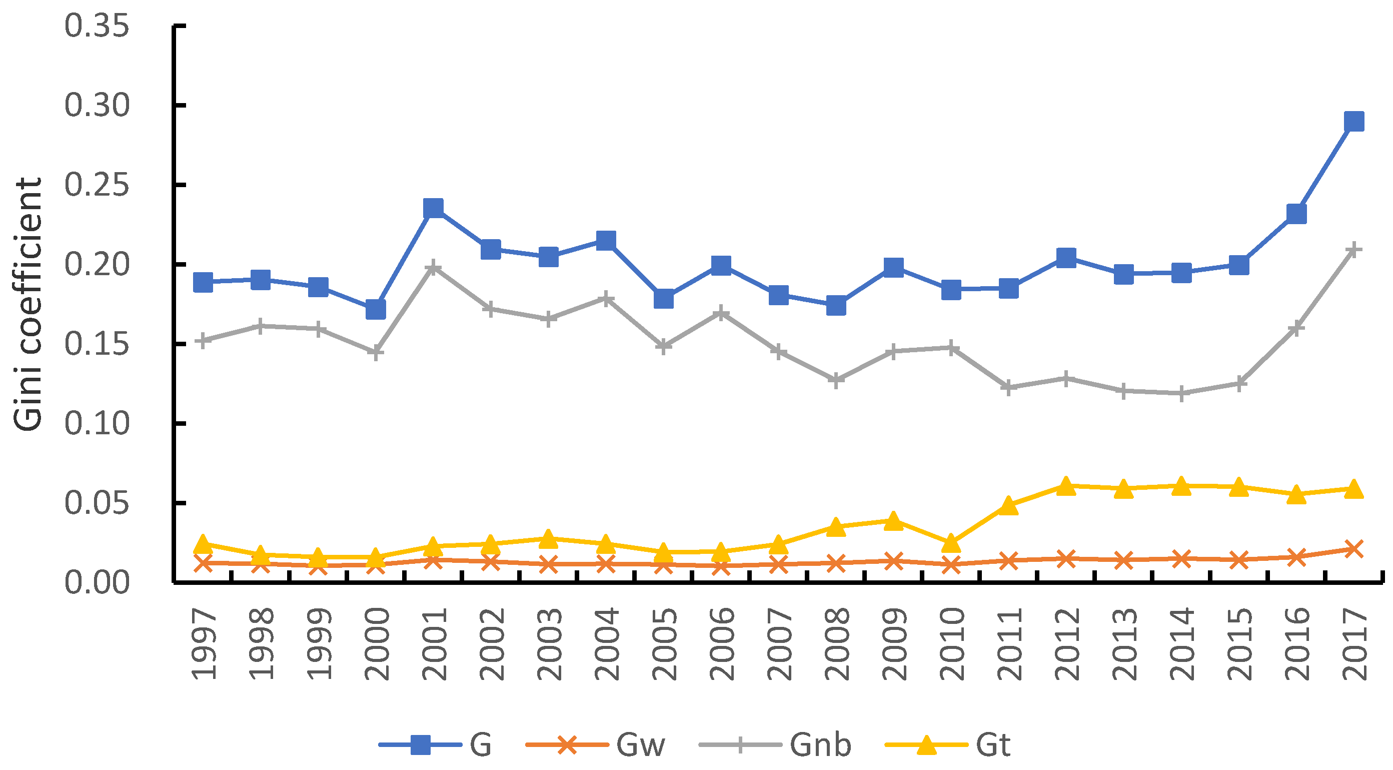
In terms of the total Gini coefficient, over the past 21 years, the total Gini coefficient of GDPI has shown a W shape. The total Gini coefficient of green development performance showed a downward trend from 1997 to 2000 and from 2001 to 2008. It indicates that the regional differences in China’s GDPI gradually became smaller during these two periods. The total Gini coefficient increased significantly in 2000–2001 and 2009–2017. In 2000 and 2001, the total Gini coefficient increased from 0.172 to 0.236. From 2009 to 2017, the total Gini coefficient increased from 0.198 to 0.290, indicating that the regional differences of green development performance in China gradually enlarged during these two periods. The year 2001 was the opening year of the Tenth Five-Year Plan. China focused on deepening the prevention and control of industrial pollution, and new or forthcoming environmental policies influenced the decisions of local industrial enterprises, resulting in a significant widening of regional differences in green development performance during the year. During the Tenth and Eleventh Five-Year Plan periods, China achieved remarkable energy conservation and emission reduction results. During the Twelfth Five-Year Plan period, China implemented a stringent environmental protection system, promulgating different policies and measures for different regions and industries. Differences in economic development levels and investments in environmental governance in different regions were observed, which led to a widening trend in the total Gini coefficient during this period. The regional differences in green development performance gradually became greater than before.
As shown in Figure 8, the evolution trend of inter-regional differences is basically consistent with that of the overall regional differences. The inter-regional differences exhibited a downward trend from 1997 to 2000, a significant increase from 2000 to 2001 and a fluctuating downward trend since 2001. Since 2000, China has been implementing an overall regional development strategy; that is, the full-scale development of the western region starting in 2000, the revitalization of the old industrial bases in the northeast in 2003, the rise of the central region in 2005, and the transformation and upgrading of the eastern region in 2008. These strategies have contributed to the narrowing of regional disparities in China since 2000. From 1997 to 2017, the super-variable density showed a characteristic of “rising–falling–rising.” The Gini coefficient for intra-regional differences was relatively small, ranging from 0.010 to 0.022. The widening inter-regional differences are the primary reason for the widening of overall difference. The average value of inter-regional differences was 0.152 from 1997 to 2017, which is significantly higher than the 0.035 from the super-variable density source and 0.013 from the intra-regional source. From the perspective of the contributions of different sources (Figure 9), the mean value of inter-regional differences is 76.01%, which is significantly higher than the mean value of 17.42% of the contribution of super-variable density and 6.57% of the contributions of intra-regional differences, indicating that inter-regional differences are primary factors influencing the overall regional differences. By contrast, super-variable density and intra-regional differences were ranked second and third, respectively.
3.2.2. Intra-Regional Differences
The evolutionary trend of intra-regional differences can reflect the degree of difference in provinces’ green development performance within economic regions. Figure 10 depicts the evolution of intra-regional differences in green development performance in the eight economic regions. Such differences in their GDPIs show fluctuating changes, with the northwest and the southern coast showing the changing characteristics of rising then falling and rising again; specifically, the northwest fluctuated greatly from 2006 to 2011. The intra-regional differences of the two regions increased significantly in 2011. The intra-regional difference in the northeast continued to decline from 2002 to 2012, but trended upward after that. The intra-regional differences in eastern coastal areas declined significantly from 1997 to 2001, indicating that the differences in the green development performance of the three eastern coastal provinces gradually became smaller during this period. After 2002, the change was relatively stable, and a substantial increase was observed in 2017. Intra-regional differences remained low in the northern coast, except for 2008 and 2009. The intra-regional differences in southwest China showed a fluctuating downward trend from 1997 to 2017, indicating that green development performance differences decreased in the five provinces in southwest China. The intra-regional differences in the middle Yellow River and the middle Yangtze river showed a fluctuating and increasing trend from 1997 to 2017. From 1997 to 2017, the mean value of intra-regional differences in green development performance in the northwest was the largest, 0.223; followed by the middle Yellow River, southwest, northeast, southern coast, the middle Yangtze River, and eastern coast, with the mean values of 0.152, 0.134, 0.111, 0.1, 0.071, and 0.06, respectively. The mean value of intra-regional differences in the northern coast was the smallest, at only 0.041. The regional differences in green development performance were the largest in the northwest and the smallest on the north coast. When formulating coordinated regional development policies in the new period, special attention should be paid to the trend of expanding regional differences in green development performance in the northwest, southern coast, the middle Yellow River, and northeast regions.
3.2.3. Inter-Regional Differences
Table 4 shows the annual average value of inter-regional Gini coefficients, denoted as , reflecting the inter-regional differences in the green development performance of China’s eight economic regions. The annual mean values of inter-regional differences between northwest and south coast, north coast, east coast, middle Yellow River, middle Yangtze River, southwest, and northeast are 0.453, 0.429, 0.408, 0.351, 0.346, 0.327, and 0.299, respectively. The annual means of inter-regional differences between the eastern and northern coasts, the southern and northern coasts, and the southern and eastern coasts are 0.076, 0.112, and 0.136, respectively. The difference between the green development performance of northwest and other regions is the largest, whereas the regional differences in the green development performance of coastal regions are relatively small.
In summary, the overall difference in China’s green development performance showed a trend of phase change from 1997 to 2017. Regional differences in green development performance expanded rapidly from 2015 to 2017, with inter-regional differences being the main reason for the expansion of overall regional differences. From 1997 to 2017, except for the southwest region, the intra-regional differences in the seven other economic regions expanded. The differences in green development performance between the northern, eastern, and southern coastal regions are relatively small. The differences in green development performance between the northwest and the seven other economic regions are large. The key to narrowing the regional gap in green development performance is to narrow the inter-regional differences.
3.3. Green Development Performance Convergence Mechanism
3.3.1. σ Convergence
The magnitude of σ convergence coefficient can reflect whether the green development performance of economic regions converges or not. As illustrated in Figure 11, the σ convergence coefficient of the nation increased from 0.342 in 1997 to 0.626 in 2017, indicating that no σ convergence characteristic of green development in the nation. The overall difference of green development level in the country tends to widen, consistent with the previous analysis. From each economic region, the σ convergence coefficients of green development in the northern coastal, northeastern, middle Yellow River, southern coastal, northwestern, and middle Yangtze River economic regions generally showed a fluctuating upward trend from 1997 to 2017. Notably, the σ convergence coefficient of green development in the eastern coastal economic region rose from 0.107 in 2016 to 0.686 in 2017, and the green development gap within the economic region expanded significantly. The σ convergence coefficient of the southwest economic region decreased from 0.314 in 1997 to 0.257 in 2017, indicating σ convergence in green development in the southwest economic region, that is, the gap in green development within the southwest economic region has a tendency to narrow.
3.3.2. β Convergence
Table 5 shows the regression results of β absolute convergence. The coefficients of β convergence are significantly positive for the whole country and the eight economic regions, indicating no absolute convergence in green development performance. That is, provinces with low green development performance do not have a catch-up effect on provinces with high green development performance. The regional gap in green development performance is widening nationwide.
Table 6 presents the regression result of β conditional convergence. After controlling control variables, such as technology level, industrial structure, energy structure, and opening to the outside world, the coefficient of β convergence for the whole country and the eight economic regions is still positive, indicating no β conditional convergence in green development performance.
4. Discussions and Conclusions
4.1. Discussions
In the past decades, urbanization in China has prioritized the coastal regions over the central and western regions. This unbalanced regional economic development strategy has laid the foundation for varying spatial green development patterns of overall high and low green development performances in the east and west regions. At present, the spatial imbalance of green development in both regions hinders China’s green development. Yet, this research area remains underexplored. The spatial imbalance pattern of economic development in Pakistan is similar to that of China. It has resulted from differences in natural conditions, transportation, government support, and investment in the east and west regions [42]. The cumulative causation laws’ intrinsic force exacerbates regional differences in economic development between China and Pakistan. Public policies also play an essential role in the emergence of regional imbalances [43].
The results show that inter-regional differences lead to regional differences in China’s green development performance. The annual average contribution of inter-regional differences to overall regional differences is as high as 76.01%. Breaking through the administrative barriers between regions, building a cross-regional cooperation mechanism for green development, and promoting green technologies’ spatial spillover are useful measures to reduce the imbalance of green development performance. Specifically, strengthening the interaction among enterprises, universities, and research institutions and develop targeted policy measures within the regional innovation system framework to promote regional green development [44]. The regional innovation system benefits from the concentration of economic activities and geographical proximity [45,46]. Finally, building comparative advantages related to the region’s unique resources with cooperation between enterprises, universities, and research institutions in provinces within the economic region can improve the region’s green development level [47].
From 1997 to 2017, the overall level of green development in China showed a slight downward trend. Although the contribution of environmental governance efficiency to green development performance has climbed year by year in recent years, it still has much room for improvement. The negative effect of economic development on the environment is an important challenge for national, regional, and local policymakers in developing sustainable development strategies [48]. As for environmental pollution, the green economy concept advocates pollution emission reduction and low-carbon economic development [49]. This proposition’s essence is still to solve environmental problems with technological innovation and progress [50]. Therefore, the regional and central government should invest in innovation to improve the country’s environmental governance efficiency and level of green development. Establishing a technological innovation system with deep integration of enterprises, universities, and research institutions can also accelerate the pace of combating environmental problems.
On the basis of the two-stage network super-efficiency SBM model and Dagum’s decomposition of the Gini coefficient, this study quantitively analyzes the level of green development and the degree of regional difference in China’s eight economic regions from 1997 to 2017. We measure the convergence on green development performance in such regions. The results are useful to deepen the theory of balanced regional development by revealing regional imbalance in eight economic regions in the country and analyzing its reasons. They can guide the overall promotion of national green development and intensive use of resources and economic transformation and upgrading. They are also a new path reference for other developing countries to follow a sustainable development path. However, this study has some limitations. We only analyze the intra-regional differences in economic regions at the provincial level rather than using prefecture-level cities. We also fail to explore the influencing factors of green development performance. Future research can look into these factors to provide further suggestions for green development paths.
4.2. Conclusions
First, from 1997 to 2017, the overall level of China’s green development performance showed a slight downward trend. Although the contribution of environmental governance efficiency to green development efficiency has climbed year by year, it still has much room for improvement.
Second, China’s regional green development performance varies significantly. The green development performance of coastal areas is significantly higher than in inland areas. Economic production efficiency and environmental governance efficiency are also higher in the east region than in the west region. The northwest region’s green development performance is significantly lower than that of the other seven economic regions and is an object that needs further investigations.
Third, the phase change is evident in terms of the overall differences in China’s green development performance. From 2015 to 2017, the overall Gini coefficient of green development performance tends to rise significantly, indicating that the regional imbalance of China’s green development performance has increased. At the same time, inter-regional differences widen the overall difference in green development performance. The northwest region has an enormous difference in green development performance. By contrast, the northern coastal region has the smallest internal difference in green development performance.
Fourth, among the eight regions, only the southwest region had σ convergence in green development performance. Moreover, absolute and conditional β convergences are divergent, thereby confirming the regional imbalance of the widening regional differences in China’s green development performance.
Author Contributions
Conceptualization, S.W. and H.W.; methodology S.W. and Y.Z.; data curation, Y.Z.; writing, S.W. and Y.Z.; supervision, H.W. All authors have read and agreed to the published version of the manuscript.
Funding
This research was funded by project of National Natural Science Foundation (41861025, 42061026) and 2019 Jiangxi Province Postgraduate Quality Course Construction “Ecological Economy and Sustainable Development”.
Institutional Review Board Statement
Not applicable.
Informed Consent Statement
Not applicable.
Data Availability Statement
The data presented in this study are available on request from the corresponding author.
Conflicts of Interest
The authors declare no conflict of interest.
References
- Jin, P.; Peng, C.; Song, M. Macroeconomic uncertainty, high-level innovation, and urban green development performance in China. China Econ. Rev. 2019, 55, 1–18. [Google Scholar] [CrossRef]
- Li, L.; Hu, J. Ecological total-factor energy efficiency of regions in China. Energy Policy 2012, 46, 216–224. [Google Scholar] [CrossRef]
- Wen, H.; Lee, C. Impact of fiscal decentralization on firm environmental performance: Evidence from a county-level fiscal reform in China. Environ. Sci. Pollut. Res. 2020, 27, 36147–36159. [Google Scholar] [CrossRef] [PubMed]
- Iftikhar, Y.; Wang, Z.; Zhang, B.; Wang, B. Energy and CO2 emissions efficiency of major economies: A network DEA approach. Energy Econ. 2018, 147, 197–207. [Google Scholar] [CrossRef]
- Kortelainen, M. Dynamic environmental performance analysis: A Malmquist index approach. Ecol. Econ. 2008, 64, 701–715. [Google Scholar] [CrossRef]
- Jena, P.R. Estimating environmental efficiency and Kuznets curve for India. In Proceedings of the Contributed Paper Prepared for Presentation at the International Association of Agricultural Economists Conference, Beijing, China, 16–22 August 2009. [Google Scholar]
- Su, S.; Zhang, F. Modeling the role of environmental regulations in regional green economy efficiency of China: Empirical evidence from super efficiency DEA-Tobit model. J. Environ. Manag. 2020, 261, 110227. [Google Scholar]
- Liu, X.; Yang, X.; Guo, R. Regional Differences in Fossil Energy-Related Carbon Emissions in China’s Eight Economic Regions: Based on the Theil Index and PLS-VIP Method. Sustainability 2020, 12, 2576. [Google Scholar] [CrossRef] [Green Version]
- Lu, C.; Venevsky, S.; Shi, X.; Wang, L.; Wright, J.S.; Wu, C. Econometrics of the environmental Kuznets curve: Testing advancement to carbon intensity-oriented sustainability for eight economic zones in China. J. Clean. Prod. 2020, 283, 124561. [Google Scholar] [CrossRef]
- Chen, Y.; Yang, Z.; Shu, F.; Hu, Z.; Meyer, M.; Bhattacharya, S. A patent based evaluation of technological innovation capability in eight economic regions in PR China. World Patent Inf. 2009, 31, 104–110. [Google Scholar] [CrossRef]
- Xie, X.; Cai, W.; Jiang, Y.; Zeng, W. Carbon footprints and embodied carbon flows analysis for China’s eight regions: A new perspective for mitigation solutions. Sustainability 2015, 7, 10098–10114. [Google Scholar] [CrossRef] [Green Version]
- Qing, Y.; Wan, X.; Ma, H. Assessing Green Development Efficiency of Municipalities and Provinces in China Integrating Models of Super-Efficiency DEA and Malmquist Index. Sustainability 2015, 7, 4492–4510. [Google Scholar]
- An, Q.; Wu, Q.; Li, J.; Xiong, B.; Chen, X. Environmental efficiency evaluation for Xiangjiang River basin cities based on an improved SBM model and Global Malmquist index. Energy Econ. 2019, 81, 95–103. [Google Scholar] [CrossRef]
- Wang, Z.; Wang, X.; Liang, L. Green economic efficiency in the Yangtze River Delta: Spatiotemporal evolution and influencing factors. Ecosyst. Health Sustain. 2019, 5, 20–35. [Google Scholar] [CrossRef] [Green Version]
- Zhao, P.; Zeng, L.; Lu, H.; Zhou, Y.; Hu, H.Y.; Wei, X.Y. Green economic efficiency and its influencing factors in China from 2008 to 2017: Based on the super-SBM model with undesirable outputs and spatial Dubin model. Sci. Total Environ. 2020, 741, 140026. [Google Scholar] [CrossRef] [PubMed]
- Cui, Y.; Liu, W.; Khan, S.U.; Yu, C.; Jun, Z.; Yue, D.; Zhao, M. Regional differential decomposition and convergence of rural green development efficiency: Evidence from China. Environ. Sci. Pollut. Res. 2020, 27, 22364–22379. [Google Scholar]
- Xu, S.; Li, Y.; Tao, Y.; Wang, Y.; Li, Y. Regional Differences in the Spatial Characteristics and Dynamic Convergence of Environmental Efficiency in China. Sustainability 2020, 12, 7423. [Google Scholar] [CrossRef]
- Wang, D.; Wan, K.; Yang, J. Ecological efficiency of coal cities in China: Evaluation and influence factors. Nat. Hazards 2019, 95, 363–379. [Google Scholar] [CrossRef]
- Li, H.; Fang, K.; Yang, W.; Wang, D.; Hong, X. Regional environmental efficiency evaluation in China: Analysis based on the Super-SBM model with undesirable outputs. Math. Comput. Model. 2013, 58, 1018–1031. [Google Scholar] [CrossRef]
- Wu, D.; Wang, Y.; Qian, W. Efficiency evaluation and dynamic evolution of China’s regional green economy: A method based on the Super-PEBM model and DEA window analysis. J. Clean. Prod. 2020, 264, 121630. [Google Scholar] [CrossRef]
- Peng, Y.; Chen, Z.; Lee, J. Dynamic Convergence of Green Total Factor Productivity in Chinese Cities. Sustainability 2020, 12, 4883. [Google Scholar] [CrossRef]
- Charnes, A.; Cooper, W.; Rhodes, E. Measuring the efficiency of decision-making units. Eur. J. Oper. Res. 1978, 2, 429–444. [Google Scholar] [CrossRef]
- Tone, K. A slacks-based measure of efficiency in data envelopment analysis. Eur. J. Oper. Res. 2001, 130, 498–509. [Google Scholar] [CrossRef] [Green Version]
- Tone, K. A slacks-based measure of super-efficiency in data envelopment analysis. Eur. J. Oper. Res. 2002, 143, 32–41. [Google Scholar] [CrossRef] [Green Version]
- Loikkanen, H.A.; Susiluoto, I. An Evaluation of Economic Efficiency of Finnish Regions by DEA and Tobit Models; 42st Congress of the European Regional Science Association: Dortmund, Germany, 2002. [Google Scholar]
- Fare, R. Measuring Farrell efficiency for a firm with intermediate inputs. Acad. Econ. Pap. 1991, 19, 329–340. [Google Scholar]
- Fare, R.; Grosskopf, S. Productivity and intermediate products: A frontier approach. Comput. Econ. 1996, 50, 65–70. [Google Scholar] [CrossRef]
- Zhu, B.; Zhang, M.; Zhou, Y.; Wang, P.; Sheng, J.; He, K.; Wei, Y.M.; Xie, R. Exploring the effect of industrial structure adjustment on interprovincial green development efficiency in China: A novel integrated approach. Energy Policy 2019, 134, 110946. [Google Scholar] [CrossRef]
- Tao, X.; Wang, P.; Zhu, B. Provincial green economic efficiency of China: A non-separable input–output SBM approach. Appl. Energy 2016, 171, 58–66. [Google Scholar] [CrossRef]
- Zhou, L.; Zhou, C.; Che, L.; Wang, B. Spatio-temporal evolution and influencing factors of urban green development efficiency in China. J. Geogr. Sci. 2020, 30, 724–742. [Google Scholar] [CrossRef]
- Peng, G.; Zhang, X.; Liu, F.; Ruan, L.; Tian, K. Spatial–temporal evolution and regional difference decomposition of urban environmental governance efficiency in China. Environ. Dev. Sustain. 2020, 1–17. [Google Scholar] [CrossRef]
- Dagum, C. A new approach to the decomposition of the Gini income inequality ratio. Empir. Econ. 1997, 22, 515–531. [Google Scholar] [CrossRef]
- Xiong, H.; Lan, L.; Liang, L.; Liu, Y.; Xu, X. Spatio-temporal Differences and Dynamic Evolution of PM2. 5 Pollution in China. Sustainability 2020, 12, 5349. [Google Scholar] [CrossRef]
- Han, H.; Ding, T.; Nie, L.; Hao, Z. Agricultural eco-efficiency loss under technology heterogeneity given regional differences in China. J. Clean. Prod. 2020, 250, 119511. [Google Scholar] [CrossRef]
- Lu, X.; Kuang, B.; Li, J. Regional difference decomposition and policy implications of China’s urban land use efficiency under the environmental restriction. Habitat Int. 2018, 77, 32–39. [Google Scholar] [CrossRef]
- Shen, C.; Feng, R.; Yu, B.; Liao, Z. Industrial CO2 Emissions Efficiency and its Determinants in China: Analyzing Differences across Regions and Industry Sectors. Pol. J. Environ. Stud. 2018, 27, 1239–1253. [Google Scholar] [CrossRef]
- National Bureau of Statistics of China (NBSC). Chinese Statistics Yearbook; NBSC: Beijing, China, 1998–2018. (In Chinese)
- National Bureau of Statistics of China (NBSC). Chinese Energy Statistics Yearbook; NBSC: Beijing, China, 1998–2018. (In Chinese)
- National Bureau of Statistics of China (NBSC). China Environment Statistics Yearbook; NBSC: Beijing, China, 1998–2018. (In Chinese)
- Rezitis, A. Agricultural productivity and convergence: Europe and the United States. Appl. Econ. 2010, 42, 1029–1044. [Google Scholar] [CrossRef] [Green Version]
- Lu, X.; Xu, C. The difference and convergence of total factor productivity of inter-provincial water resources in China based on three-stage DEA-Malmquist index model. Sustain. Comput. Inform. Syst. 2019, 22, 75–83. [Google Scholar] [CrossRef]
- Sobhan, R. The Problem of regional imbalance in the economic development of Pakistan. Asian Surv. 1962, 2, 31–37. [Google Scholar] [CrossRef]
- Toprak, M.; Bayraktar, Y.; Özyılmaz, A. Analysis of the Impact of Public Investments on Regional Imbalance at the Regional Level in Turkey; International Congress on Politic, Economic and Social Studies (ICPESS): Istanbul, Turkey, 2017. [Google Scholar]
- Doloreux, D.; Parto, S. Regional innovation systems: Current discourse and unresolved issues. Technol. Soc. 2005, 27, 133–153. [Google Scholar] [CrossRef]
- Doloreux, D. What we should know about regional systems of innovation. Technol. Soc. 2002, 24, 243–263. [Google Scholar] [CrossRef]
- Isaksen, A.; Trippl, M. Exogenously led and policy-supported new path development in peripheral regions: Analytical and synthetic routes. Econ. Geogr. 2017, 93, 436–457. [Google Scholar] [CrossRef]
- Maillat, D.; Kebir, L. Conditions-cadres et compétitivité des régions: Une relecture. Can. J. Reg. Sci. 2001, 24, 41–56. [Google Scholar]
- Rockström, J.; Steffen, W.; Noone, K.; Persson, Å.; Chapin, F.S.; Lambin, E.F.; Lenton, T.M.; Scheffer, M.; Folke, C.; Schellnhuber, H.J.; et al. A safe operating space for humanity. Nature 2009, 461, 472–475. [Google Scholar] [CrossRef] [PubMed]
- Davies, A.; Mullin, S. Greening the economy: Interrogating sustainability innovations beyond the mainstream. J. Econ. Geogr. 2011, 11, 793–816. [Google Scholar] [CrossRef]
- Mol, A. Ecological modernization and the global economy. Glob. Environ. Politics 2002, 2, 92–115. [Google Scholar] [CrossRef]
Figure 1.
Economic production and environmental governance efficiency transformation system for green development performance.
Figure 1.
Economic production and environmental governance efficiency transformation system for green development performance.

Figure 2.
Map of Chinese provinces with green development performance scores.

Figure 3.
Comparison of green development performance and sub-link efficiency from 1997 to 2017.

Figure 4.
Comparison of the green development performance of eight economic regions from 1997 to 2017. Note: 1, 2, 3, 4, 5, 6, 7, and 8 represent the northern coast, northeast, eastern coast, middle Yellow River, southern coast, northwest, southwest, and middle Yangtze River, respectively.
Figure 4.
Comparison of the green development performance of eight economic regions from 1997 to 2017. Note: 1, 2, 3, 4, 5, 6, 7, and 8 represent the northern coast, northeast, eastern coast, middle Yellow River, southern coast, northwest, southwest, and middle Yangtze River, respectively.

Figure 5.
Spatial patterns of green development performance in 1997 (a) and 2017 (b).

Figure 6.
Radar charts for economic production and environmental governance efficiency measurements.
Figure 6.
Radar charts for economic production and environmental governance efficiency measurements.

Figure 7.
Spatial patterns of economic production efficiency (a) and environmental governance efficiency (b).
Figure 7.
Spatial patterns of economic production efficiency (a) and environmental governance efficiency (b).

Figure 8.
Evolution trend of the sources of regional differences in green development performance from 1997 to 2017.
Figure 8.
Evolution trend of the sources of regional differences in green development performance from 1997 to 2017.

Figure 9.
Changes in the contribution rates of regional differences in green development performance from 1997 to 2017.
Figure 9.
Changes in the contribution rates of regional differences in green development performance from 1997 to 2017.

Figure 10.
Trends of intra-regional differences in the eight economic regions from 1997 to 2017. Note: 1, 2, 3, 4, 5, 6, 7, 8 represent the northern coast, northeast, eastern coast, middle Yellow River, southern coast, northwest, southwest, and middle Yangtze River, respectively.
Figure 10.
Trends of intra-regional differences in the eight economic regions from 1997 to 2017. Note: 1, 2, 3, 4, 5, 6, 7, 8 represent the northern coast, northeast, eastern coast, middle Yellow River, southern coast, northwest, southwest, and middle Yangtze River, respectively.

Figure 11.
σ convergence analysis of green development performance of China and eight economic regions from 1997 to 2017. Note: 1, 2, 3, 4, 5, 6, 7, 8 represent the northern coast, northeast, eastern coast, middle Yellow River, southern coast, northwest, southwest, and middle Yangtze River, respectively.


Table 1.
Constitutions of China’s eight economic regions.
| Regions | Constitutions |
|---|---|
| Northern coast | Beijing, Tianjin, Hebei, Shandong |
| Eastern coast | Shanghai, Jiangsu, Zhejiang |
| Southern coast | Fujian, Guangdong, Hainan |
| Northeast | Liaoning, Jilin, Heilongjiang |
| Middle Yellow River | Shanxi, Inner Mongolia, Henan, Shaanxi |
| Middle Yangtze River | Anhui, Jiangxi, Hubei, Hunan |
| Southwest | Guangxi, Chongqing, Sichuan, Guizhou, Yunnan |
| Northwest | Ningxia, Gansu, Qinghai, Xinjiang |
Table 2.
Evaluation index system of GDPI in China.
| Stage | Type | First Level Indicators | Second Level Indicators | Third Level Indicators |
|---|---|---|---|---|
| Economic production stage | Input | Resource input | Labor | Employed persons |
| Capital | Total investment in fixed assets | |||
| Energy | Energy consumption | |||
| Water | Per capita water consumption | |||
| Land | Area of built districts | |||
| Output | Economic output | GDP | Area GDP | |
| Intermediate variable | Pollution emissions | Wastewater | Total wastewater discharged | |
| Waste gas | SO2 emission | |||
| Solid waste | Industrial solid waste discharge | |||
| Environmental governance stage | Input | Environmental governance | Environmental input | Investment in the treatment of environmental pollution |
| Output | Waste utilization | Wastes utilization | Facilities for treatment of waste water and waste gas | |
| Waste water utilization | Treat of industrial wastewater | |||
| Solid waste utilization | Utilization of solid waste |
Table 3.
Pearson correlation analysis between GDPI, GPE, and GEE.
| GDPI | GPE | GEE | |
|---|---|---|---|
| GDPI | 1 | 0.941 *** | 0.798 *** |
| GPE | 0.941 *** | 1 | 0.777 *** |
| GEE | 0.798 *** | 0.777 *** | 1 |
Note: *** represents significant levels of 1%.
Table 4.
Average annual inter-regional Gini coefficients for green development performance in the eight economic regions.
Table 4.
Average annual inter-regional Gini coefficients for green development performance in the eight economic regions.
| Region | Region | Region | Region | ||||
|---|---|---|---|---|---|---|---|
| 8-7 | 0.148 | 7-6 | 0.327 | 6-4 | 0.351 | 5-1 | 0.112 |
| 8-6 | 0.346 | 7-5 | 0.246 | 6-3 | 0.408 | 4-3 | 0.156 |
| 8-5 | 0.190 | 7-4 | 0.171 | 6-2 | 0.299 | 4-2 | 0.179 |
| 8-4 | 0.144 | 7-3 | 0.193 | 6-1 | 0.429 | 4-1 | 0.168 |
| 8-3 | 0.133 | 7-2 | 0.172 | 5-4 | 0.206 | 3-2 | 0.205 |
| 8-2 | 0.135 | 7-1 | 0.218 | 5-3 | 0.136 | 3-1 | 0.076 |
| 8-1 | 0.155 | 6-5 | 0.453 | 5-2 | 0.264 | 2-1 | 0.228 |
Note: 1, 2, 3, 4, 5, 6, 7, 8 represent the northern coast, northeast, eastern coast, middle Yellow River, southern coast, northwest, southwest, middle Yangtze River, respectively.
Table 5.
Green development performance β absolute convergence regression results.
| Region | β | t | Constant | t | R2 |
|---|---|---|---|---|---|
| Nationwide | 0.285 *** | 5.18 | 0.0382 | 1.31 | 0.0778 |
| Northern Coast | 0.619 *** | 48.18 | −0.0832 | −2.27 | 0.4433 |
| Northeast | 0.265 ** | 5.78 | 0.0373 | −0.43 | 0.3927 |
| Eastern coast | 0.780 * | 4.16 | 0.0748 | 0.40 | 0.2223 |
| The Middle Yellow River | 0.395 * | 3.05 | 0.0429 | 0.64 | 0.2589 |
| Southern coast | 0.183 ** | 5.12 | −0.0139 | −0.51 | 0.4581 |
| Northwest | 0.209 * | 2.53 | 0.183 | 1.41 | 0.4001 |
| Southwest | 0.383 *** | 4.82 | 0.158 | 2.03 | 0.2081 |
| The Yangtze River | 0.647 *** | 10.02 | −0.0960 | −1.19 | 0.3980 |
Note: ***, **, * represent significant levels of 1%, 5% and 10%, respectively.
Table 6.
Green development performance β conditional convergence regression results.
| Region | β | t | Constant | t | R2 |
|---|---|---|---|---|---|
| Nationwide | 0.289 *** | 5.54 | −0.160 | −0.31 | 0.0714 |
| Northern Coast | 0.670 *** | 13.15 | −0.800 | −1.03 | 0.3586 |
| Northeast | 0.425 * | 2.93 | −2.746 * | −3.29 | 0.1405 |
| Eastern coast | 0.936 ** | 9.56 | 1.218 | 0.75 | 0.1718 |
| The Middle Yellow River | 0.404 | 2.18 | −1.727 | −1.13 | 0.1883 |
| Southern coast | 0.188 | 2.53 | −0.646 | −0.37 | 0.4055 |
| Northwest | 0.305 | 2.03 | −1.046 | −0.33 | 0.2601 |
| Southwest | 0.498 *** | 5.39 | −0.742 | −1.22 | 0.2738 |
| The Yangtze River | 0.721 *** | 9.46 | 2.472 | 0.92 | 0.3791 |
Note: ***, **, * represent the significant levels of 1%, 5%, and 10%, respectively. Due to space constraints, the results of control variables are not listed.
Publisher’s Note: MDPI stays neutral with regard to jurisdictional claims in published maps and institutional affiliations. |
© 2021 by the authors. Licensee MDPI, Basel, Switzerland. This article is an open access article distributed under the terms and conditions of the Creative Commons Attribution (CC BY) license (http://creativecommons.org/licenses/by/4.0/).
Share and Cite
MDPI and ACS Style
Wang, S.; Zhang, Y.; Wen, H. Comprehensive Measurement and Regional Imbalance of China’s Green Development Performance. Sustainability 2021, 13, 1409. https://0-doi-org.brum.beds.ac.uk/10.3390/su13031409
AMA Style
Wang S, Zhang Y, Wen H. Comprehensive Measurement and Regional Imbalance of China’s Green Development Performance. Sustainability. 2021; 13(3):1409. https://0-doi-org.brum.beds.ac.uk/10.3390/su13031409
Chicago/Turabian StyleWang, Shengyun, Yaxin Zhang, and Huwei Wen. 2021. "Comprehensive Measurement and Regional Imbalance of China’s Green Development Performance" Sustainability 13, no. 3: 1409. https://0-doi-org.brum.beds.ac.uk/10.3390/su13031409
Note that from the first issue of 2016, this journal uses article numbers instead of page numbers. See further details here.