Article

Through the Irregular Paths of Inequality: An Analysis of the Evolution of Socioeconomic Inequality in Brazilian States Since 1976 †

by
Paulo Mourao
1,* and
Alexandre Junqueira
2
1
School of Management and Economics & NIPE, Minho University, 4710-057 Braga, Portugal
2
School of Management and Economics, Minho University, 4710-57 Braga, Portugal
*
Author to whom correspondence should be addressed.
Authors acknowledge the contribution of two anonymous reviewers on a previous version of this research. Remaining limitations are authors’ exclusive ones.
Sustainability 2021, 13(4), 2356; https://0-doi-org.brum.beds.ac.uk/10.3390/su13042356
Submission received: 29 January 2021 / Revised: 9 February 2021 / Accepted: 17 February 2021 / Published: 22 February 2021
(This article belongs to the Special Issue Economic Development and Inequality: The Role of Cities and Regions)

Abstract

:
Patterns of inequality tend to seriously undermine any attempt at economic growth policy when the inequality is perceived by significant groups of individuals as unjust, inhuman, and insurmountable. One country with a high degree of inequality has been Brazil (usually in the world top-10). Brazil had also witnessed strong dynamics of certain indicators, such as the Gini coefficient, over the last several decades. However, so far, such dynamics have not been properly analyzed, especially considering the significant differences across Brazilian states. For filling that gap, this study used econometric techniques specific to time series and tried to identify structural breaks in the series of Gini coefficients for the 27 Brazilian states since 1976. Results showed a tendency towards an increase in inequality until 1995, followed by a reduction in inequality since 2000. Some cases of Brazilian states were related to the absence of structural breaks, showing a maintenance of historical trends in the evolution of inequality, which raises important policies’ challenges.

1. Introduction

The issue of socioeconomic inequality—how certain resources in a community are concentrated in clusters of that community—has been a theme in economic and political debates for most societies since World War II. Although combating inequality is often second to the priority of economic growth, the negative consequences of socioeconomic inequality are evident and are themselves a significant brake on the economic growth of each country as well as that of neighboring economies.
Inequality of income and resources in Brazil has been a concern of scholars since it first began to be measured, detailed, and debated. It has been a concern for more than fifty years. This work will revisit this long debate, from pioneering authors such as Josué de Castro and Celso Furtado, but bringing the focus to a reality hitherto worked with little detail: the possible existence of several Kuznets cycles in the inequality indicators observed for both the Brazilian federation and each state.
Additionally, our work will observe the presence of inflection points in the evolution of the Gini coefficients, both for Brazil and within each of the 27 states. We will carry out this investigation using official data since 1976, given the robustness of the data available from that point of initial observation.
For this purpose, we will use econometric techniques associated with time series, focused on the identification of structural breaks, identifying the moments of change in the evolution of the Gini coefficient observed for each state [1].
The structure of this work is as follows: beyond the Introduction section, Section 2 will revisit the literature—both national and international—on economic inequality and will culminate in three hypotheses, tested here. Hypothesis 1 follows [2], who defended the existence of a single Kuznets cycle to explain the evolution of inequality in countries like Brazil since the end of World War II. Hypothesis 2 follows [3] who defended differences between states in terms of endogenous evolutions in patterns of socioeconomic inequality. Hypothesis 3 is supported by [4] who, contrary to authors who defend a single Kuznets cycle, propose shorter cycles of reactions/interactions between federal and state policies and spontaneous expressions of inequality (such as in [5]) which overlap the single Kuznets cycle. Subsequently, Section 3 will empirically test these hypotheses and discuss them. Finally, Section 4 will present conclusions, implications derived from this work, and opportunities for future research.

2. Literature Review

2.1. From Pareto and Kuznets to Josué de Castro and Celso Furtado—The Evolution of Inequality and Its Distribution among the Brazilian States

As studies by [6,7] showed, the evolution associated with patterns of inequality registered in a given country has different configurations. From studies of Pareto or the famous Kuznets curve (dated 1955 and inspired by Tocqueville texts) to the presence of several Kuznets curves observed in a long period of observations, many contributions have sought to analyze the patterns of inequality of a society with the evolution of economic growth or with the temporal evolution in itself [8].
As [9] has argued, the debate on inequality is often accompanied by diverse priorities as well as a certain confusion of objectives. Within the first issue—the presence of other priorities—we have a triangle of issues. This triangle is made from the dimensions of economic growth, the minimum of effective rights, and the minimum of structures available to citizens. Thus, on a political agenda, priority is given to achieving higher (and sustained) levels of economic growth and to offering citizens a minimum level of effective rights (such as minimum schooling or public health response systems in the face of medical emergencies) as well as relevant infrastructures (e.g., plumbing, electrification, media, or housing quality). Only after these objectives are achieved at levels considered politically satisfactory does the problem of inequality between social groups and within the same groups currently become an important issue on the political agenda. Regarding confusion of objectives, Ref [9] refers to the confusion in many public debates between inequality and absolute poverty/wealth, between income inequality and consumption inequality, and between inequality of usufruct and inequality of power.
However, several authors—from [9] to [8]—warn of the consequences of these inequalities. Ref [10] believe that inequality compromises the economic growth process itself. This argument is seconded by authors like [8], who claim that inequalities tend to endure and reproduce, functioning as a significant factor to explain the different rates of economic growth worldwide. We will revisit this debate in the following paragraphs.
If originally the bell figure of a Kuznets curve suggests that the pattern of inequality increased up to a given inflection point observed in relation to both economic growth and the temporal trend, the works of [11] claim this figure has been stretched over time, assuming the presence of several bells. In the genesis, and looking at the interpretations of [6,8], inequality in extremely poor societies is usually very low, because the population’s incomes are equally low and their destiny is focused on subsistence consumption. As industrialization progresses, there is the mobility of workers from the lowest-paid sectors (agriculture and other branches of the so-called primary sector) to the highest-paid sectors (such as industry). Given the heterogeneity specific to the various tasks associated with the industry, Kuznets suggested the presence of differentiated remuneration in societies based on industrialization, which led to greater inequality in distributed remuneration as well as in associated living conditions. At a later stage, with the development of welfare states with redistributive mechanisms (such as a progressive tax system), inequality tends to decrease, leading to the famous Kuznets hypothesis of an inverted U associating inequality with development.
The various empirical tests launched to test the Kuznet curve (or Kuznet curves) have given few encouraging results if a universal law was sought. Little by little, control factors were attached to the bivariate relationship of origin—namely, financial liquidity, the volume, and composition of public expenditures, the opening of the economy, age structure, etc. Clear results were generally achieved for limited sample countries and for defined periods.
In Latin America, as [8] reports, there was a certain approximation of the average income in recent decades, but there is still great inequality within countries. The lowest inequality for countries in the region is in Uruguay (Gini coefficient of 0.45), with the highest inequality patterns in Brazil and Bolivia, with Gini coefficients above 0.60.
Other authors like [12] discuss the majority of Latin American countries as spaces influenced by the persistence of low wages despite technological capacity, which led them to receive foreign direct investment without the capacity to raise local wages, a more evident phenomenon since the 1960s. [12] further details the composition of the work of these countries (characterized by the prevalence of low salaries but with high technological capacity), identifying high densities in rural populations, and with a significant population of artisanal and industrial producers limited to the local market, as well as an urban population with strong stimuli left to informal sectors and concentrated on employees of the exporting industry and new entrepreneurs.
Ref [13] has also detailed the impact of dynamics of sub-spaces in the dynamics of inequality observed for all spaces. It was evident that changes in inequality within each space will lead to changes in global inequality. Alternatively, in the discussion of global inequality, the works of [14,15] showed that global inequality tends to decrease when more unequal sub-spaces have higher growth rates, especially sub-spaces whose residents have lower per capita incomes.
Among the works that clearly elucidate the correlations between socioeconomic inequality and a diversity of indicators is that of [10]. The authors draw various correlations between patterns of inequality and a great diversity of socioeconomic dimensions, ranging from crime and latent violence to patterns of schooling.

2.2. About the Gini Coefficient

The advantages and limitations of using the Gini coefficient as a metric for inequality patterns of an economy have already been discussed and detailed to a great extent [16,17,18]. Proposed by a contemporary of Vilfredo Pareto—the Italian Corrado Gini—the Gini coefficient compares each person’s income with the income of everyone individually, and the sum of all bilateral income differences is divided by the number of individuals included in the calculation. The resulting Gini coefficient ranges from 0 (absolute equality) to 1 (where all earnings are in the hands of a single holder). As [8] outlines, Gini coefficients between 0.25–0.3 are found in the most egalitarian countries (like some Nordic countries, the Czech Republic and Slovakia, and also cases like Cuba and Liberia, according to [19]) while values around 0.6 are common in countries such as Brazil and South Africa.
The dynamics surrounding the progression of the Gini coefficient have been discussed for most of the countries observed. For example, the evolution of the respective progression in the United States of America was rather unique. Authors like [8] showed that inequality in the United States of America decreased until the end of the 1970s when it reached a value of 0.35. Since that time, the value has continued to rise. But this increase was seconded by countries like China or Russia. The European Union itself has maintained Gini coefficients around 0.4.
Other authors [8,15] suggest the introduction of superior details to the calculation to understand the sources of inequality—whether it is due to the inequality between groupings of society or space (between-components), or to inequality within each grouping (within-components). Authors who contributed to the argument of inequality between societal groups include [20,21]; in contrast, authors like [22,23] address inequality within groups. Thus, studies focusing on inequality have reinforced the need to look for inequality within each region, or in the case of a federal country, for inequalities within each state as well as the respective evolution. In reality, as [8] claimed, inequality—if viewed as the responsibility of individuals—requires social policies for individuals, regardless of states/spaces; if inequality is viewed as the responsibility of localization, it requires differentiated social policies.
Given our intention to study the inequality observed in the states of Brazil, we will now detail the reality of the socioeconomic differentiation of the 27 states in the next section.

2.3. The Situation of Brazil in This Debate

Socioeconomic inequality in Brazil gave rise to a vast study that, without neglecting previous contributions, emerged with its own cadence from authors such as [24,25,26].
To [24], social inequality was a reality that affected individuals and groups in its fullness, a vision that [25] believe still continues today. If [24] started with a structuralist vision in his studies before 1960, he later understood how inequality not only manifests in the differentiation of calorie patterns ingested by individuals, but also affects the same individuals in all dimensions of human participation. It proposes structural development plans that would affect all Brazilian states, focusing on the development of agriculture and subsequently on other sectors of activity.
In contrast, Refs [25,27]—in [28] and following [29]—argues that the unequal distribution of income in Brazil is the result of a distributive tacit agreement between the economic and political power of social classes. Under the ECLAC center-periphery debates from 1948, Ref [25] calls for a new South American political generation, capable of combating (from within) the inequality of Latin American states, depressed by stages of latent underdevelopment (meaning that even growing in terms of production and income, they are not successful in reducing inequality). As a consequence of regional and state inequalities, Furtado suggests that these inequalities converged in a poverty of opportunities, hope, and access—that is, poverty under different dimensions, approaching the holistic reading of Josué de Castro [25,28].
Income inequality in Brazil thus has special nuances. Authors such as [8,30] have shown that Brazil currently covers the spectrum of world distribution—having citizens living with some of the smallest incomes in the world but also having citizens with some of the highest incomes in the world. As [8] shows, a fifth of the Brazilian population is better off than the poorest Americans.
Brazil, with improvements to its economy, witnessed an inclusive growth process until 2014. This allowed an improvement in the GINI index and brought 26.5 million Brazilians out of poverty. However, in recent years a decline in these indicators has been reported. Social inclusion started to grow but was interrupted and, since 2014, extreme poverty has increased by 40%, as a result of a combination of falling income, unemployment, and increased inequality [31].
According to the World Bank classification, Brazil is classified among countries with medium-high income, based on the Gross National Income (GNI) per capita. By that criterion, the poverty line is bounded below $5.50 PPP. In 2018, there were 52.5 million people living in poverty in Brazil, with incomes below US $5.50 PPP per day, approximately R $420 per month (this number corresponds to 25.3% of the population). The number of people living in extreme poverty was 13.5 million, with a per capita monthly income of less than R $145, or US $1.9 per day, which is the World Bank’s classification of extreme poverty [32].
Until the 1930s, the hunger felt by individuals living in many Brazilian states was the greatest reflection of inequality; only after the crisis of 1929 did Brazilian agriculture start to diversify and increase the supply of basic necessities to its population. From the 1930s to the end of the 1980s, the government began to control distribution and set prices to try to offer better living conditions to the poorest people.
The 1980s became known as the “lost decade” [33], marked by an increase in poverty and an overall economic decline. It was a period accompanied by an increase in the degree of inequality, where average income fell and inequality grew, causing social welfare to decline. In this period, the average income of the richest 20% increased from 63 to 65%, while the average income of the poorest 50% decreased from 14% in 1980 to 12% in 1990. Despite this “lost decade,” the responsibility of the state in social assistance appeared for the first time in the 1988 Constitution; at that time, governments were required to guarantee a minimum level of security and income for all citizens. In line with the Constitution, some federal income distribution programs—such as the Continuous Payment Benefit (BPC) and Rural Social Security (PSR)—were created with the objective of protecting vulnerable social groups, such as the elderly and people with disabilities who have limited ability to work. BPC works through non-contributory transfers, guaranteeing minimum resources for basic consumption, while PSR serves informal workers, giving them access to social security (Barrientos, 2013).
Socioeconomic inequality also increased from 0.597 in 1980 to 0.603 in 1990. In the same period, the percentage of families with an income below the minimum wage increased from 20.8% in 1979 to 26.5% in 1990 [34]. Since the height in 1990, there has been a gradual reduction to the most recent date (2018), with a value of 0.53.
Poverty and social inequality in Brazil in the 1980s were studied by several authors, based on the diagnosis of Hélio Jaguaribe and his team. In 1987, the government proposed a government action plan which aimed to benefit 73 million people. Among the measures envisaged were the doubling of the purchasing power of the minimum wage and a food supplement for 60 million Brazilians [35].
At the beginning of the 1990s, with the economy opening, the government believed that deregulating the market would provide greater incomes, emancipate poor families, and improve the realization of citizenship rights [36].
During the 1990s, two important civil society actions redesigned the landscape of fighting inequality and hunger in Brazil. The first was the creation of Pastoral da Criança, an ecumenical entity that aimed to eradicate child malnutrition, by Bishop Dom Evaristo Arns and his sister Zilda Arns. The second came from Herbert de Souza, who in 1993 started a campaign that would profoundly mark the new direction of the fight against hunger in the country. Citizenship Action Against Hunger, Poverty, and for Life—which gained the approval of society as a whole as well as the federal government—was a movement to fight hunger and included a recommendation to create a Food Security Council. The Council was created under the acronym CONSEA and was led by Bishop Dom Paulo Morelli. During the tenure of President Fernando Henrique Cardoso, CONSEA was abolished and actions to combat hunger were taken over by first lady Ruth Cardoso. Only in 2003, with the election of Lula da Silva as president, did CONSEA resume [37].
Citizenship Action Against Hunger, Poverty, and for Life was such an inspiring campaign that many other entities joined forces, and a movement that was initially focused only on fighting hunger expanded to spotlight poverty as a whole. Over time, even entities that emerged to combat hunger have improved and expanded their focus of action.
In 2003, with the rise of the Workers’ Party, social programs gained strength under the administration of President Luiz Inácio Lula da Silva, and the first action of the new executive was the creation of the Zero Hunger Program. This program was implemented after the creation of the Extraordinary Ministry of Food Security (MESA), which aimed to formulate and coordinate the implementation of a National Food and Nutrition Security Policy. However, after only a year, this Ministry was extinguished and replaced by the Ministry of Social Development and Fight against Hunger (MDS). This action intended to spotlight the convergence of government actions aimed at social inclusion, the fight against hunger, the eradication of poverty, and social inequalities [38].
Although the state’s social policies were established by the 1988 Constitution, it was only in the 1990s that public policies to combat poverty began to emerge. In 1992 the federal government instituted the Minimum Income Guarantee Program; in 1993, the Continuous Service Benefit was implemented, in 1996, the Child Labor Eradication Program, and in 1995, the Solidarity Economy Program. In the early 2000s, these programs were expanded and reformed. In 2001 the Bolsa-Escola, the Bolsa Comida, and the Auxílio-Gás were created, in 2003, the Food and Zero Hunger Card were created. In October of the same year, the unification and remodeling of all these programs resulted in the Bolsa Família Program, instituted on 9 January 2004 [39].
According to [40], Bolsa-Escola was intended for low-income families with children between 6 and 15 years old, while Bolsa-Comida benefited those with children up to age 7. The operation of both programs was identical, targeting families with per capita income below half the minimum wage; both were associated with public health and education programs and the transfer of funds was made directly to the beneficiary via a magnetic card. Both benefits had the same value of R $15 per child, limited to three benefits per family. Under Auxílio-Gás, the benefit was R $7.5/month, targeting low-income families whose members earned per capita income of up to half of minimum wage per month.
According to a survey by [40], these programs were not effective at reducing poverty or misery. Bolsa-Escola was the most effective, considering the sum of the results achieved. Bolsa-Food and gas assistance had a very small impact on its target groups: only 1.5 million people were impacted, which represented 1% of the vulnerable population at the time [40].
In October 2003, through Provisional Measure No. 132, converted into Law 10,386/2004, the Bolsa Família Program (PBF) was created, as a result of the merger of many of the previously mentioned programs. The objective of this union was to reduce administrative expenses, based on coordinated and integrated intersectoral management, configuring itself as a direct income transfer program [38]. This action was only possible thanks to the creation of the Cadastro Único (“CadÚnico”), which was the instrument that identified and characterized low-income families, allowing the government to better understand the socioeconomic realities of this population.
Social investment increased in Brazil during the period between 1980 and 2010, from 13% of the gross domestic product (GDP) in the 1980s to almost 25% in 2010. These findings can also be observed in the work of [24] or of [27]. According to [30], we can consider the Continuous Payment Benefit (BPC), the rural retirement benefit, and Bolsa Família (PBF) as the three major federal income transfer programs (currently worth around 4% of Brazilian GDP).
From 1993 to 2010, 60 million people migrated from low-income (classes D and E) to middle-income classes (class C). This result is partly due to income distribution programs such as Bolsa Família, but also to the demographic change in Brazil, such as fewer children and the elderly and more people of working age.
Souza [30] analyzed the Brazilian income tax data from 1926 to 2015 to measure inequality and evidence the concentration of wealth at the top of the social pyramid. According to the author, the fluctuation in the concentration of Brazilian income coincides with historical political moments. Since 1920, Brazil registered an increase in the concentration of income, reaching its peak in the years 1942–1943, during the Vargas dictatorship; after that, there was a slight decline, but it returned to growth in the 1960s, with the new dictatorial regime. Even with the re-democratization in the 1980s, inequality continued to grow, and although there has been a reduction since the 1990s, expressed by the Gini coefficient, the data indicate that at the top of the pyramid, there was no impact and, therefore, the redistribution essentially occurred only among the 90% of the middle classes, without affecting the richest 10%. Also, [30] points out that the concentration of Brazilian income in the past was lower than in rich countries, but the difference widened after the second war.
De Mendonça et al. [41] detailed several empirical analyzes on inequality and income for the five Brazilian macro-regions. The study by [41] compared the Gini and Theil indexes and the income ratio of the richest 10% with the poorest 40% between 1999 and 2008. The results show that the South was the region with less inequality while the Northeast had the worst performance. For the authors, some factors help to explain the fall in Brazilian inequality in this period, among them, the commercial opening, the real increase in the minimum wage, the technological and financial development, the reduction of unemployment, and the Bolsa Família program. However, factors such as the shift in political power and increased social spending did not impact inequality. On the other hand, corruption had a positive correlation with the increase in inequality.
According to [42], as a continental country, Brazil faces serious problems of regional inequalities, which were originated in the late 19th century but still persist. Although projects have appeared overtime to promote the development and integration of Brazilian regions, these initiatives have never managed to mitigate such differences. According to [42], these differences are the result of the lack of a long-term development project. These Regional inequalities must be understood as imbalances/disparities in the rates of economic growth in different areas of the country, which means that regardless of the indicator, the North and Northeast regions tend to present the worst rates, while the South and Southeast tend to show the better growth rates. Although there has been an improvement in recent decades, the disparities remain. The problem arises from industrial and, later, financial centralization in the South/Southeast regions, and even though the Federal Constitution (1988) stipulated the adoption of a national integration project, until now, such policy has not been implemented and has not prevented the intensification of regional inequalities.

2.4. Intra-State Inequality in Brazil

If, as seen, the evolution of the Gini coefficient for the Brazilian federation had these periods identified (growth over the 1980s, maximum peak in 1990 with a coefficient of 0.63, and a gradual reduction until today, with a value of 0.53 in 2018), it is important to detail the different evolution of each state.
The states with the maximum value of the Gini coefficient in the period 1976 to 2018 were Espírito Santo (maximum 0.658 in the Gini coefficient in 1988), Amapá (maximum 0.658 in 1993–1994), and Paraíba (maximum 0.656 in 1999–2000). In contrast, the states with the lowest values in the same period and considering IBGE (2018) as source were Roraima (0.393, in 1983), Santa Catarina (0.409, in 2014), and Amapá (0.429, in 1989).
If we look at the standard deviation calculated for the Gini coefficients between 1976 and 2018, the states with the highest deviations were Amapá (standard deviation of 0.054), Piauí (standard deviation of 0.051), and Santa Catarina (standard deviation of 0.047). This demonstrates that there was a marked dynamic of inequality patterns measured for these states over these four decades.
The states with the lowest deviations—and therefore with the most stable Gini coefficients—were the states of Brasília (Distrito Federal) with a standard deviation of 0.018, São Paulo (standard deviation of 0.018), and Rio de Janeiro (deviation of 0.029).
Considering the most recent available work [3], the least unequal Brazilian cities and their Gini coefficients are:
  • São José do Hortêncio (in the state of Rio Grande do Sul, RS) 0.28
  • Botuverá (Santa Catarina, SC) 0.28
  • Alto Feliz (RS) 0.29
  • São Vendelino (RS) 0.29
  • Vale Real (RS) 0.29
  • Santa Maria do Herval (RS) 0.30
  • Tupandi (RS) 0.31
  • Campestre da Serra (RS) 0.31
  • Nova Pádua (RS) 0.32
  • Córrego Fundo (in the state of Minas Gerais) 0.32
  • Santa Rosa de Lima (SC) 0.32
  • Picada Café (RS) 0.32
  • President Lucena (RS) 0.32
  • Vila Flores (RS) 0.32
  • Morro Reuter (RS) 0.32
A report from 2020 [43] details the Gini índex for each state capital in Brazil considering the income distribution:
  • Recife (0.605)
  • João Pessoa (0.587)
  • São Paulo (0.581)
  • Vitória (0.573)
  • Aracaju (0.573)
  • Fortaleza (0.566)
  • Palmas (0.562)
  • Boa Vista (0.556)
  • Macapá (0.552)
  • Rio de Janeiro (0.552)
  • Porto Alegre (0.547)
  • Belo Horizonte (0.545)
  • Maceió (0.535)
  • Natal (0.534)
  • São Luís (0.531)
  • Curitiba (0.525)
  • Manaus (0.523)
  • Rio Branco (0.518)
  • Teresina (0.511)
  • Campo Grande (0.507)
  • Florianópolis (0.476)
  • Goiânia (0.475)
Just for comparison, the most recent value available for Brasilia (the Federal capital) has been provided by [44] and it is 0.628 (for the year of 2010).
Figure A1 (at Appendix A) details the evolution of the Gini coefficient for the 27 Brazilian states since 1976. Overall, checking Figure A1 and the previous ranks, we follow the suggestions of [41,42] the socioeconomic inequality tends to be more severe in North and Northeast regions while the socioeconomic inequality tends to be reduced in South and Southeast regions.

2.5. Literature Synthesis and Working Hypotheses

We can summarize the positioning of the various currents in view of the evolution of inequality in Brazil as follows:
Tucker [2] defends the existence of a single Kuznets cycle to explain the evolution of inequality in countries like Brazil since the end of World War II;
Narloch [3] defends differences between states in terms of endogenous changes in patterns of socioeconomic inequality;
Caldeira [4], contrary to authors who defend a single Kuznets cycle, proposes shorter cycles of reactions/interactions between federal policies and spontaneous expressions of inequality (as in [45]); these short cycles overlap the single Kuznets cycle and are periodically delimited.
Summarizing the literature review with the evidence discovered so far, three hypotheses emerge:
Hypothesis 1 (H1).
Brazil, unlike the original modeling of the Kuznets curve, has had several Kuznets cycles. This hypothesis implies phases of growth of inequality followed by phases of mitigation.
Hypothesis 2 (H2).
As a result of state and federal endogenous dynamics, combined with state and federal policies, different states experienced different dynamics in terms of socioeconomic inequality.
Hypothesis 3 (H3).
There are specific and short cycles for each state.

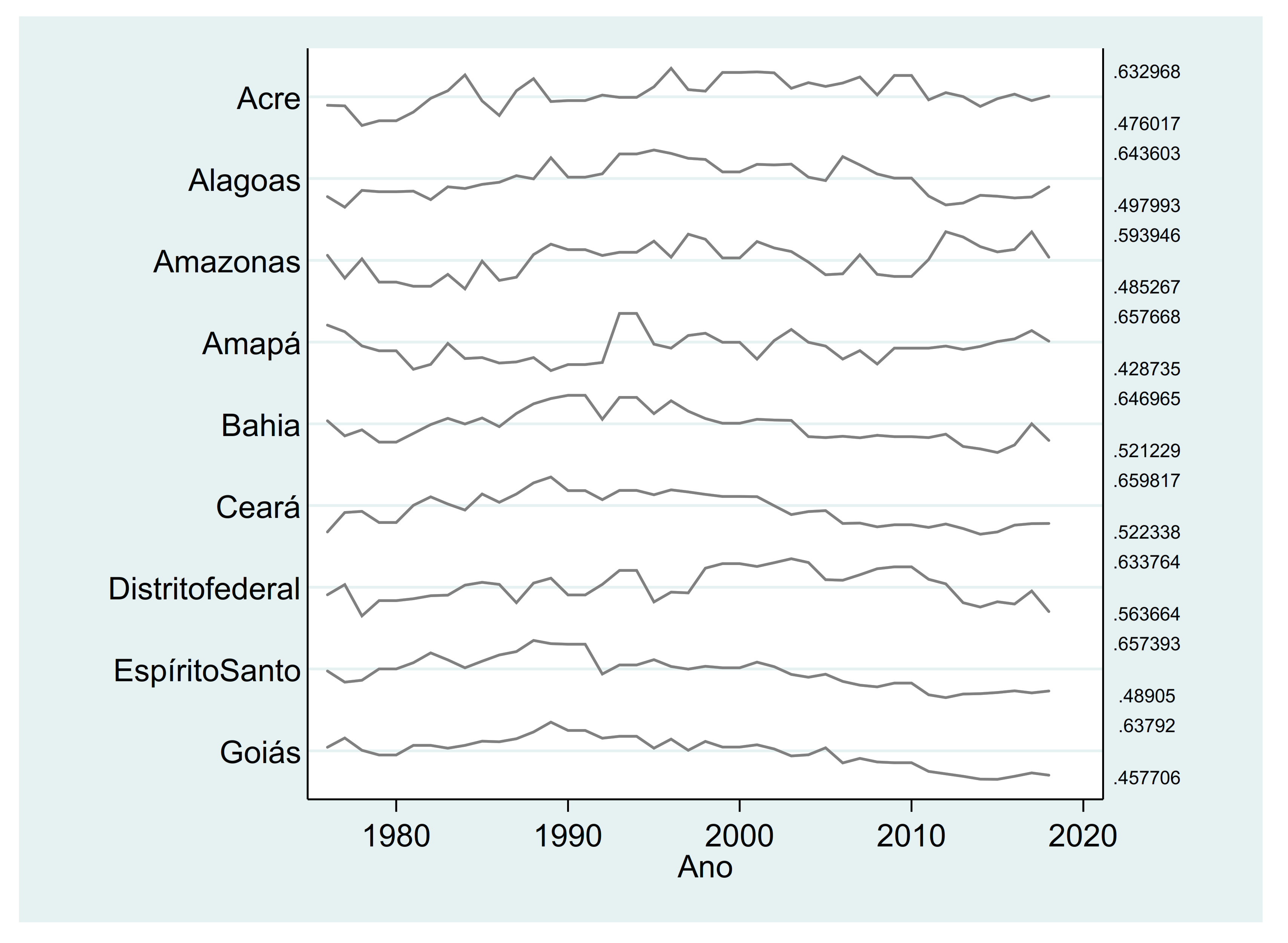
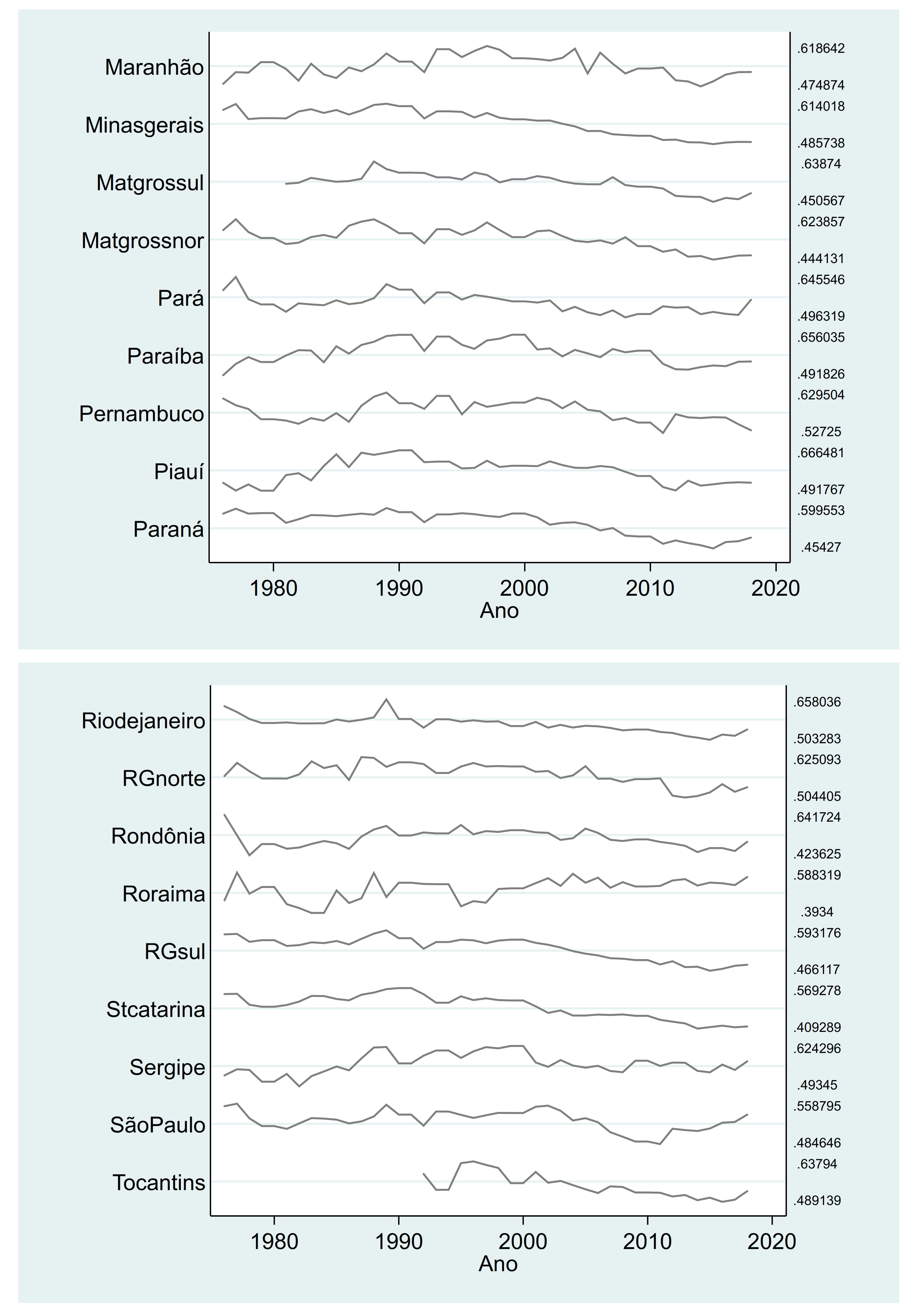
3. Empirical Section—Testing Breaks in Brazilian Series for Gini Coefficient

To test the existence of structural breaks in the series related to the Gini index computed for each Brazilian state for the years 1976–2018, we will identify multiple time breaks.
As [46] states, “The history of the analysis of structural breaks in time series is well documented in works like Aue and Horvath (2013 [47]) or Lu and Ito (2008 [48]). From the first generations, focused on testing the statistical significance of structural breaks identified for precise moments (like the Chow test), we now have tests for unknown dates. Within these modern tests, we find the tests for multiple time breaks, like Clemente et al. (1998 [1]), whose critical values were previously suggested by Perron and Vogelsang (1992 [49])”.
The test by [1] led us to analyze the nature of the break, differentiating between sudden breaks in the series (“additive outliers”) or smooth changes (“innovational outliers”). [50] noted that tests like that of [1] have additional convenience properties because they do not impose so many restrictions on the stationarity of the series as tests like [51] that imposed, for instance, that the series must be I(0); i.e., stationary at levels.
Using the forms of [52], we will identify bt to each series of the Gini index computed for each Brazilian state between 1976 and 2018. To test the presence of multiple additive outliers, we estimate the following system using Equation (1):
b t = α + δ 1 D U 1 t + δ 2 D U 2 t + e t e t = i = 1 k w 1 i D T b 1 , t i + i = 1 k w 2 i D T b 2 , t i + ρ e t i + i = 1 k θ i Δ e t i + z t
DU1t = 1 for the year t after the first break time and zero, otherwise. Equivalently, DU2t is equal to 1 for the time observation t after the second break time and zero, otherwise. Tb1 and Tb2 identify the break points to be analyzed by grid search (i.e., by identifying the minimal t-ratio for the hypothesis ρ = 1). Following [52], we use DTbm,t = 1 for t = Tbm + 1 and 0 for m = 1, 2.
To test ρ = 1 with the presence of innovational outliers, we will analyze the model provided by Equation (2) ([52]):
b t = α + δ 1 D U 1 t + δ 2 D U 2 t + w 1 D T b 1 , t + w 2 D T b 2 , t + α b t i + i = 1 k θ i Δ b t i + z t
As previously suggested, our series were collected from the official source [32]. Descriptive statistics are available in Table 1. Columns 1–4 in Table 2 show the results from the tests conducted by [1] on the observed series.

Discussion of Results

Looking at Table 2 and Table A1 (at Appendix A), we see that, for most Brazilian states in the 1976-2018 period, two moments of structural breakdown were identified. For the majority of states, the first structural breakdown was identified primarily between 1984 and 1995, and was positive and statistically significant, which shows that the majority of Brazilian states saw an increase in socioeconomic inequality during this period, which converges with the insight of [41,53]. The second structural breakdown, concentrated mainly between 1999 and 2012, was negative and again statistically significant, reflecting a decrease in socioeconomic inequality in various states. We considered that a moment was a structural break if validated simultaneously by the tests considering statistically significant for results by AO and IO.
We suggest paying attention to the cases of Pará—in which only one significant break was identified—or the example of Amazonas—which had no significant structural breaks. In the first group of special cases, it is evident that these states maintained the dynamics of increased socioeconomic inequality that started before 1980 through the 1990s, with only a break in this dynamic during the first decade of 2000. In the second group of special cases, these states have not yet significantly changed the dynamics observed in the evolution of the Gini index since first observed.
Considering cases with two structural changes—that is, with 3 or 4 moments identified as statistically significant in the 4 analyzed moments (two per AO and two per IO)—we observed that the majority of the cycles between breaks had an average duration of 10 years. This reinforces the claim in Hypothesis 3, the existence of short cycles composing the longer national Kuznets cycle.

4. Conclusions

This work reflected on the evolution of socioeconomic inequality in one of the most emblematic countries, Brazil. Considered a traditional example of an unequal country, with millions of residents earning low incomes, Brazil is also simultaneously a country with elite populations earning some of the highest incomes worldwide. In addition, the evolution of general patterns of inequality has decreased over the past two decades in Brazil.
We deepened this analysis, focusing on the dynamics observed within each of the 27 states since 1976. Through an econometric analysis of time series, we identified moments for each state of structural breaks, associated with moments when the previous (increasing or decreasing) trend has been changed, especially in the opposite direction.
In general, two moments of the structural break were identified. For most states, the first moment was identified mainly between 1984 and 1995, was positive and statistically significant, which shows that the majority of Brazilian states saw increased socioeconomic inequality during this period. The second moment, concentrated largely between 1999 and 2012, was negative and again statistically significant, reflecting a decrease in the patterns of socioeconomic inequality in various states.
The richness of this work does not end here. Despite this relevant contribution to the framing of endogenous inequality in Brazilian states, questions emerge about the causes that may have fueled these movements and the implications to the lives of citizens. If in one way, an implication of this work is related to verifying the different dynamics of the states within the larger national dynamic, in another way, the analysis of the reconciliation of state policies with federal policies can lead to more stimulating results—for example, a better understanding of why the rhythms of evolution of inequality were so different across Brazilian states, without neglecting the role of internal migrations, the role of changes in the active population, or the evolution of the population’s educational patterns.
Although the debate on inequality seems devalued in the face of the dilemma regarding growth vs. equalization—that is, must we prioritize the growth of the country or promote greater equity in the distribution of resources and income?—we believe that the debate is necessary. Patterns of inequality tend to seriously undermine any attempt at economic growth policy when the same inequality is perceived by individuals as unjust, inhuman, and insurmountable.

Author Contributions

Conceptualization: P.M. and A.J.; methodology, P.M. and A.J.; software, P.M.; validation, P.M., A.J.; formal analysis, P.M.; investigation, P.M. and A.J.; resources, P.M.; data curation, P.M.; writing—original draft preparation, P.M. and A.J.; writing—review and editing, P.M.; visualization, P.M.; supervision, P.M.; project administration, P.M.; funding acquisition, P.M. All authors have read and agreed to the published version of the manuscript.

Funding

This paper is financed by National Funds of the FCT–Portuguese Foundation for Science and Technology within the project “UIDB/03182/2020”.

Institutional Review Board Statement

Not applicable.

Informed Consent Statement

Not applicable.

Data Availability Statement

Data will be provided if requested to Authors.

Conflicts of Interest

The authors declare no conflict of interest.

Appendix A

Figure A1. Evolution of Gini Coefficient across Brazilian states. Note: Ano (Year).
Sustainability 13 02356 g0a1aSustainability 13 02356 g0a1b
Table A1. Identification of breaks for each state’s Gini coefficients.
States Diminishing InequalityYearsStates Increasing Inequality
1980
1981
1982
1983
1984Amazonas, Baía, Ceará, Paraíba, Pernambuco, Rondônia, Sergipe
1985
1986Alagoas, Roraima
1987
1988
1989
1990Amapá, Maranhão,
1991
1992
1993Acre, Espírito Santo,
1994
St Catarina1995Brasília DF
1996Goiás
1997
1998
Amapá, MG Sul1999
Minas Gerais, Pará, RG Norte2000
Baía, MG, Tocantins2001
Paraíba, São Paulo2002
Ceará, Paraná, RG Sul, St Catarina, Sergipe2003
Maranhão, Pernambuco2004
2005
2006
Goiás, Piauí2007
Alagoas, Espírito Santo, Minas Gerais, Rio, Rondônia2008
MG Sul, MG, Paraná2009
RG Norte, RG Sul2010
Tocantins2011
Acre, Brasília DF2012
2013
2014
2015

References

  1. Acemoglu, D. Technical Change, Inequality, and the Labor Market; NBER Working Paper: Cambridge, UK, 2000. [Google Scholar]
  2. Acemoglu, D.; Robinson, J.A. The Political Economy of the Kuznets Curve. Rev. Dev. Econ. 2002, 6, 183–203. [Google Scholar] [CrossRef]
  3. Arize, C.A.; Bakarezos, P.; Kallianiotis, I.N.; Malindretos, J.; Phelan, J. The Gini Coefficient: An Application to Greece. Int. J. Econ. Finance 2018, 10, 205–214. [Google Scholar]
  4. Aue, A.; Horváth, L. Structural breaks in time series. J. Time Ser. Anal. 2012, 34, 1–16. [Google Scholar] [CrossRef]
  5. Bai, J.; Perron, P. Critical values for multiple structural change tests. Econ. J. 2003, 6, 72–78. [Google Scholar] [CrossRef]
  6. Barros, R.P.; Mendonça, R.S.; Duarte, R.P. Bem-Estar, Pobreza e Desigualdade de Renda: Uma Avaliação da Evolução Histórica e das Disparidades Regionais. IPEAr; pp. 1–59. 1997. Available online: http://repositorio.ipea.gov.br/bitstream/11058/1992/1/td_0454.pdf (accessed on 14 April 2020).
  7. Baum, C. Stata: The language of choice for time-series analysis? Stata J. 2005, 5, 46–63. [Google Scholar] [CrossRef] [Green Version]
  8. Belik, W.; Da Silva, J.G.; Takagi, M. Políticas de combate à fome no Brasil. São Paulo Perspec. São Paulo em Perspect. 2001, 15, 119–129. [Google Scholar] [CrossRef] [Green Version]
  9. Caldeira, J. História da Riqueza no Brasil; Estação Brasil: Rio de Janeiro, Brazil, 2017. [Google Scholar]
  10. Castro, J. Geopolítica da Fome; Casa do Estudante do Brasil: Rio de Janeiro, Brazil, 1951. [Google Scholar]
  11. Cidades, S. Mapa Da Desigualdade Entre As Capitais Brasileiras—2020. Brasília, 2020. Available online: https://www.cidadessustentaveis.org.br/arquivos/link/mapa-das-desigualdades.pdf (accessed on 12 February 2021).
  12. Clemente, J.; Montañés AReyes, M. Testing for a unit root in variables with a double change in the mean. Econ. Lett. 1998, 59, 175–182. [Google Scholar] [CrossRef]
  13. Costa, A.C.; Kerstenetzky, C.L. Desigualdade intragrupos educacionais e crescimento. Econ. E Soc. 2005, 14, 337–364. Available online: https://periodicos.sbu.unicamp.br/ojs/index.php/ecos/article/view/8643031 (accessed on 12 February 2021).
  14. Diniz, C.C. Celso Furtado e o desenvolvimento regional. Nova Econ. 2009, 19, 227–249. [Google Scholar] [CrossRef]
  15. Lima, F.; Cristovao, L. The Persistent Inequality in the Great Brazilian Cities: The Case of Brasília; MPRA Paper 50938; University Library of Munich: Munich, Germany, 2013. [Google Scholar]
  16. Souza, P.H. A History of Inequality: Top Incomes in Brazil, 1926–2015. Res. Soc. Strat. Mobil. 2018, 57, 35–45. [Google Scholar] [CrossRef] [Green Version]
  17. Furtado, C. Intra-country discontinuities: Towards a theory of spatial structures. Inf. (Int. Soc. Sci. Counc.) 1967, 6, 7–16. [Google Scholar] [CrossRef]
  18. Furtado, C. Brasil: A Construção Interrompida; Paz e Terra: Rio de Janeiro, Brazil, 1992. [Google Scholar]
  19. Galor, O.; Moav, O. Ability biased technological transition, wage inequality and growth. Q. J. Econ. 2000, 115, 469–497. [Google Scholar] [CrossRef] [Green Version]
  20. Gezycy, F. New Regional Definition and Spatial Analysis of Regional Inequalities in Turkey Related to the Regional Policies of EU; ERSA Congress Proceedings: Oporto, Portugal, 2004. [Google Scholar]
  21. Giraud, P.-N. A Desigualdade do Mundo—A Economia do Mundo Contemporâneo; Terramar: Lisboa, Portugal, 1996. [Google Scholar]
  22. Gould, E.; Moav, O.; Weinberg, B. Precautionary Demand for Education, Inequality, and Technological Progress. J. Econ. Growth 2001, 6, 285–315. [Google Scholar] [CrossRef]
  23. Graham, M. Disaggregation of the Gini Coefficient and Its Application to Australia 1986. In Economic Analysis and Policy; Elsevier: Amsterdam, The Netherlands, 1995; Volume 25, pp. 140–151. [Google Scholar]
  24. Hayek, F.A. Studies in Philosophy, Politics and Economics; Touchstone: New York, NY, USA, 1969; p. 97. [Google Scholar]
  25. Horwitz, S. Monetary Evolution, Free Banking, And Economic Order; Routledge: New York, NY, USA, 2019. [Google Scholar]
  26. IBGE. Síntese de Indicadores Sociais: Uma Análise das Condições de Vida da População Brasileira 2019. Estudos e Pesquisas Informação Demográfica e Socioeconômica, 2019. pp. 1–134. Available online: https://biblioteca.ibge.gov.br/visualizacao/livros/liv101678.pdf (accessed on 13 April 2020).
  27. do Jannuzzi, P.; Pinto, A.R. Bolsa Família e seus Impactos nas Condições de vida da População Brasileira: Uma Síntese dos Principais Achados da Pesquisa de Avaliação de Impacto do Bolsa Família II; Ipea: Brasília, Brazil, 2012. [Google Scholar]
  28. Campello, E.T.; Neri, M.C. Programa Bolsa Família: Uma Década de Inclusão e Cidadania; Ipea: Brasília, Brazil, 2013; pp. 181–192. [Google Scholar]
  29. Krueger, A. How computers have changed the wage structure: Evidence from microdata, 1984–1989. Q. J. Econ. 1993, 108, 33–60. [Google Scholar] [CrossRef]
  30. Lu, S.Q.; Ito, T. Structural Breaks and Time-varying Parameter: A Survey with Application. Commun. IBIMA 2008, 2008, 100037. [Google Scholar]
  31. Mendez, R. Creative destruction and the rise of inequality. J. Econ. Growth 2002, 7, 259–281. [Google Scholar] [CrossRef]
  32. De Mendonça, H.F.; Esteves, D.M. Income inequality in Brazil: What has changed in recent years? CEPAL Rev. 2014, 2014, 107–123. Available online: https://repositorio.cepal.org/handle/11362/37023 (accessed on 12 February 2021). [CrossRef] [Green Version]
  33. Milanovic, B. Ter ou não ter—Uma Breve História da Desigualdade; Bertrand Editora: Lisboa, Portugal, 2012. [Google Scholar]
  34. Mourao, P. Smoking Gentlemen—How Formula One Has Controlled CO2 Emissions. Sustainability 2018, 10, 1841. [Google Scholar] [CrossRef] [Green Version]
  35. Mourao, P.; Martinho, V. Discussing structural breaks in the Portuguese regulation on forestfires—An economic approach. Land Use Policy 2016, 54, 460–478. [Google Scholar] [CrossRef]
  36. Narloch, L. Guia Politicamente Incorreto da Economia Brasileira; Leya: Rio de Janeiro, Brazil, 2015. [Google Scholar]
  37. Neri, M. Sem “norte”, Serão 15 Anos Para Brasil Voltar a Pobreza de 2014. Folha de São Paulo, 2019. Available online: https://temas.folha.uol.com.br/desigualdade-global/brasil/sem-norte-serao-15-anos-para-brasil-voltar-a-pobreza-de-2014.shtml (accessed on 19 August 2019).
  38. Ometto, A.M.; Furtuoso, M.C.; Silva, M.V. Economia Brasileira na Década de Oitenta e seus Reflexos nas Condições de vida da População. Rev. Saúde Pública 1995, 29, 1–12. [Google Scholar] [CrossRef] [PubMed] [Green Version]
  39. Paula, J. Celso Furtado e as Grandes Questões Dosub Desenvolvimento Brasileiro. X Encontro de Economia Baiana—SET. 2014. Conference Proceedings/X Encontro Economia Baiana, 2014. pp. 630–648. Available online: http://www.eeb.sei.ba.gov.br/pdf/2014/pl/celso_furtado.pdf (accessed on 12 February 2021).
  40. Perron, P.; Vogelsang, T. Nonstationarity and level shifts with an application to purchasing power parity. J. Bus. Econ. Stat. 1992, 10, 301–320. [Google Scholar]
  41. Pickett, K.; Wilkinson, R. O Espírito da Igualdade-Por que Razão Sociedades Mais Igualitárias Funcionam Quase Sempre Melhor; Editorial Presença: Lisboa, Portugal, 2010. [Google Scholar]
  42. Ponce, J. A Desigualdade é um Indicador Errado e Enganoso-Concentre-Se na Pobreza. Institute von Mises–Brazil, 2018. Available online: https://mises.org.br/ArticlePrint.aspx?id=2848 (accessed on 26 February 2018).
  43. Queiroz, S.N.; Remy, M.A.; Pereira, J.M.; Filho, L.A. Análise da Evolução dos Programas Federais de Transferência de Renda (PBF e BPC) no Brasil e Estados do Nordeste—2004–2009. XVII Encontro Nacional de Estudos Populacionais (ABEP). 2010. Available online: https://www.researchgate.net/profile/Silvana_Queiroz/publication/329591856_Analise_da_evolucao_dos_programas_federais_de_transferencia_de_renda_PBF_e_BPC_no_Brasil_e_estados_do_Nordeste-2004-2009/links/5c1198eaa6fdcc494ff020e1/Analise-da-evolucao-dos-prog (accessed on 12 February 2021).
  44. Rocha, S. Impacto sobre a Pobreza dos Novos Programas Federais de Transferência de Renda. Rev. de Econ. Contemp. 2005, 9, 153–185. [Google Scholar]
  45. Rogerson, P. The Gini coefficient of inequality: A new interpretation. In Letters in Spatial and Resource Sciences; Springer: Berlin/Heidelberg, Germany, 2013; Volume 6, pp. 109–120. [Google Scholar]
  46. Roine, J.; Waldenström, D. Long-run trends in the distribution of income and wealth. In Handbook of Income Distribution; Atkinson, A.B., Bourguignon, F., Eds.; Elsevier: Amsterdam, The Netherlands, 2015; Volume 2A. [Google Scholar]
  47. Santagada, S. A Situação Social do Brasil nos anos 80. Indicadores Econômicos FEE, 121-143. 1990. Available online: https://revistas.dee.spgg.rs.gov.br/index.php/indicadores/article/download/179/389 (accessed on 12 February 2021).
  48. da Silva, S.A. Regional Inequalities in Brazil: Divergent Readings on Their Origin and Public Policy Design. EchoGéo 2017. [Google Scholar] [CrossRef] [Green Version]
  49. Silva, M.; Nunes, E. Josué de Castro e o pensamento social brasileiro. Cad. de Saúde Colect. 2017, 22, 3677–3687. [Google Scholar] [CrossRef] [Green Version]
  50. Souza, J. A Invisibilidade da Desigualdade Brasileira; Editora UFMG: Belo Horizonte, Brazil, 2006. [Google Scholar]
  51. Souza, A.P. Políticas de Distribuições de Renda no Brasil e o Bolsa-Família. Escola de Economia de São Paulo da Fundação Getulio Vargas FGV-EESP, 1-36. 2011. Available online: https://bibliotecadigital.fgv.br/dspace/handle/10438/9995 (accessed on 12 February 2021).
  52. Tucker, J. The Market Loves You: Why You Should Love It Back; American Institute for Economic Research: New York, NY, USA, 2019. [Google Scholar]
  53. Zimmermann, C. Os Programas Sociais Sob a Ótica dos Direitos Humanos: O Caso do Bolsa Família do Governo Lula No Brasil. Sur Rev. Int. de Direitos Hum. 2006, 4, 145–161. [Google Scholar] [CrossRef] [Green Version]
Table 1. Descriptive statistics.
VariableObsMeanStd. Dev.MinMax
Acre430.5647270.0389960.4760170.632968
Alagoas430.5694350.0405570.4979930.643603
Amazonas430.5413870.0304450.4852670.593946
Amapá430.5214230.0545090.4287350.657668
Bahia430.5816840.0342480.5212290.646965
Ceará430.5835990.0377320.5223380.659817
Distritofed(Brasilia)430.6011720.0187810.5636640.633764
EspíritoSanto430.5657710.0452220.489050.657393
Goiás430.5455090.0463550.4577060.63792
Maranhão430.5479070.0380030.4748740.618642
Minasgerais430.5559920.0406220.4857380.614018
Matgrossul380.5413890.0416680.4505670.63874
Matgrossnor430.5395290.0476130.4441310.623857
Pará430.549550.0332270.4963190.645546
Paraíba430.5855750.0449630.4918260.656036
Pernambuco430.5818320.0255170.527250.629504
Piauí430.5763430.0513460.4917670.666481
Paraná430.5460.0424240.454270.599553
Riodejaneiro430.5625780.0294660.5032830.658036
RGnorte430.5741010.0312580.5044050.625093
Rondônia430.5150790.0446840.4236250.641724
Roraima430.5103740.0504710.39340.588319
RGsul430.5373450.0350960.4661170.593176
Stcatarina430.4957040.0467940.4092890.569278
Sergipe430.5666450.03320.493450.624296
SãoPaulo430.5280370.0182130.4846460.558795
Tocantins430.548570.0427930.4891390.63794
Table 2. Tests on structural breaks (Brazilian states, 1976–2018).
StateStructural Breaks—AO, Year1
[Dlt_u Coeff.]
(t-Stat)
Structural Breaks—IO, Year1
[Dlt_u Coeff.]
(t-Stat)
Structural Breaks—AO, Year2
[Dlt_u Coeff.]
(t-Stat)
Structural Breaks—IO, Year2
[Dlt_u Coeff.]
(t-Stat)
Acre1993
[0.05]
(5.15)
1980
[0.001]
(0.11)
2012
[−0.04]
(−3.02)
1993
[0.03]
(7.07)
Alagoas1986
[0.06]
(7.59)
1985
[0.04]
(3.21)
2008
[−0.06]
(−7.82)
2009
[−0.05]
(−3.7)
Amazonas1984
[0.04]
(4.06)
1986
[0.001]
(0.25)
2006
[0.003]
(0.21)
2009
[0.01]
(1.16)
Amapá1990
[0.04]
(2.61)
1991
[0.07]
(3.6)
2006
[−0.01]
(−0.77)
1999
[−0.04]
(−2.2)
Baía1984
[0.04]
(4.8)
1979
[0.03]
(2.8)
2001
[−0.05]
(−7.8)
2002
[−0.03]
(−3.6)
Ceará1984
[0.04]
(5.1)
1979
[0.001]
(0.34)
2003
[−0.07]
(−10.2)
2000
[−0.02]
(−2.76)
Brasília1995
[0.02]
(5.2)
1996
[0.02]
(3.96)
2012
[−0.03]
(−6.1)
2011
[−0.04]
(−4.39)
Espírito Santo1993
[0.03]
(3.1)
2010
[−0.02]
(−2.23)
2008
[−0.05]
(−4.9)
2005
[−0.02]
(−2.0)
Goiás1996
[0.03]
(3.5)
2001
[−0.03]
(−3.3)
2007
[−0.06]
(−6.6)
2009
[−0.02]
(−2.4)
Maranhão1990
[0.04]
(4.5)
1987
[0.04]
(3.6)
2004
[−0.06]
(−5.7)
2006
[−0.06]
(−4.5)
Minas Gerais2000
[−0.04]
(−7.6)
1997
[−0.01]
(−1.3)
2008
[−0.04]
(−5.3)
2003
[−0.01]
(−1.2)
Mato Grosso Sul1999
[−0.02]
(−2.5)
2001
[−0.02]
(−1.6)
2009
[−0.06]
(−5.9)
2010
[−0.03]
(−2.8)
Mato Grosso1986
[0.01]
(0.81)
2001
[−0.02]
(−2.3)
2006
[−0.08]
(−7.5)
2009
[−0.03]
(−2.1)
Pará1986
[0.02]
(1.6)
1988
[0.01]
(0.33)
2000
[−0.05]
(5.9)
2001
[−0.02]
(−1.3)
Paraíba1984
[0.07]
(6.1)
1985
[0.01]
(0.37)
2002
[−0.07]
(−6.9)
1999
[−0.06]
(−4.3)
Pernambuco1984
[0.02]
(4.2)
1985
[0.03]
(3.8)
2004
[−0.03]
(−6.3)
2005
[−0.04]
(−5.1)
Piauí1982
[0.08]
(7.3)
1983
[0.01]
(0.07)
2008
[−0.08]
(−7.4)
2007
[−0.04]
(−3.9)
Paraná2003
[−0.05]
(−7.6)
2000
[−0.03]
(−4.9)
2009
[−0.04]
(−6.6)
2006
[−0.03]
(−3.4)
Rio Janeiro1987
[−0.01]
(−1.3)
1988
[−0.01]
(−1.8)
2008
[−0.04]
(−5.2)
2006
[−0.02]
(−4.2)
Rio Grande Norte2000
[−0.02]
(−2.9)
2001
[−0.02]
(−2.9)
2009
[−0.04]
(−4.4)
2010
[−0.03]
(−3.3)
Rondonia1984
[0.03]
(2.7)
1985
[0.07]
(5.4)
2008
[−0.05]
(−4.1)
2007
[−0.06]
(−5.5)
Roraima1985
[0.02]
(1.5)
1987
[0.01]
(0.88)
1999
[0.04]
(2.7)
1986
[0.07]
(3.2)
Rio Grande Sul2003
[−0.05]
(−9.1)
2002
[−0.03]
(−3.7)
2010
[−0.02]
(−4.7)
2012
[−0.01]
(−1.5)
Santa Catarina1995
[−0.02]
(−2.4)
1999
[−0.03]
(−4.4)
2003
[−0.07]
(−6.7)
2009
[−0.04]
(−4.9)
Sergipe1984
[0.06]
(7.7)
1985
[0.05]
(4.7)
2002
[−0.03]
(−4.5)
1999
[−0.03]
(−4.4)
São Paulo1990
[0.01]
(1.4)
1986
[0.01]
(1.7)
2005
[−0.02]
(−5.8)
2005
[−0.01]
(−2.3)
Tocantins2001
[−0.04]
(−4.1)
2001
[−0.04]
(−2.7)
2011
[−0.03]
(−2.5)
2007
[−0.01]
(−0.92)
Publisher’s Note: MDPI stays neutral with regard to jurisdictional claims in published maps and institutional affiliations.

