
Resilience of Urban Economic Structures Following the Great Recession


1
School of Complex Adaptive Systems, Arizona State University, Tempe, AZ 85287, USA
2
Global Climate Forum, 10178 Berlin, Germany
3
Decision Theater, Arizona State University, Tempe, AZ 85287, USA
4
School of Life Sciences, Arizona State University, Tempe, AZ 85287, USA
*
Author to whom correspondence should be addressed.
Sustainability 2021, 13(4), 2374; https://0-doi-org.brum.beds.ac.uk/10.3390/su13042374
Submission received: 21 January 2021
/
Revised: 10 February 2021
/
Accepted: 18 February 2021
/
Published: 23 February 2021
(This article belongs to the Special Issue Feature Papers in Economic and Business Aspects of Sustainability)
Abstract
:The future sustainability of cities is contingent on economic resilience. Yet, urban resilience is still not well understood, as cities are frequently disrupted by shocks, such as natural disasters, economic recessions, or changes in government policies. These shocks can significantly alter a city’s economic structure. Yet the term economic structure is often used metaphorically and is often not understood sufficiently by those having to implement policies. Here, we operationalized the concept of economic structure as a weighted network of interdependent industry sectors. For 938 U.S. urban areas, we then quantified the magnitude of change in the areas’ economic structures over time, focusing on changes associated with the 2007–2009 global recession. The result is a novel method of analyzing urban change over time as well as a typology of U.S. urban systems based on how their economic structures responded to the recession. We further compared those urban types to changes in economic performance during the recession to explore each structural type’s adaptive capacity. Results suggest cities that undergo constant but measured change are better positioned to weather the impacts of economic shocks.
1. Introduction
A prerequisite for global sustainability is the sustainable transition of the world’s cities [1,2]. Such transitions are often disruptive, and cities are increasingly embracing resilience thinking as a strategy for navigating transitions [3,4]. As the authors of [5] state, “strategies for sustainable management … should focus on maintaining resilience.” Thus, resilience and sustainability are intimately related [6], and while urban resilience is required in many sectors—education, transportation, health, security, etc.—we focus here on economic resilience as a key requirement for sustainable urban futures [7,8].
However, there remains much to be understood about economic resilience [9,10]. Shocks, such as the global COVID-19 pandemic, have revealed pervasive vulnerabilities within urban economies [11,12,13,14]. These vulnerabilities arise partly through globalization and technological advances, which have created a dense global web of highly interdependent economies [15,16]. Such interdependence, or connectedness, can cause shocks to spread more widely and rapidly than they otherwise might [17]. In response, practitioners and researchers alike have turned to resilience as a framework for both understanding and managing vulnerabilities of cities during sustainability transitions [18].
Like all complex adaptive systems, cities typically reconfigure their internal structures in response to a shock or disturbance. Such structures include engineered, social, ecological, and economic structures, and how those structures change in response to a shock can give important clues about the resilience and adaptive capacity of individual cities. In this study we focused on the economic structures of 938 U.S. urban areas, examining how those structures changed in response to the 2007–2009 global recession.
This required that we first defined what we meant by economic structure. Following previous studies [19,20], we defined the economic structure of a city as a network of interdependent economic units. In this study, those economic units were individual industries. Representing complex systems as networks has long been proposed as a framework for understanding system vulnerabilities and resilience [21], and recent studies have sought to operationalize that framework by creating quantified metrics of urban resilience [22,23].
We contributed to this emerging area of scholarship, not by proposing a novel metric of resilience, but by quantifying the magnitude of change in a city’s economic structure over time before, during, and after the 2007–2009 global recession. We then used k-means clustering to identify a novel typology of cities based on how their economic structures changed over our study period of 2001–2017. For each cluster identified we calculated an archetypical response curve of structural change over time and compared that curve to the cluster’s average economic performance both during the recession period and during a recovery period. By comparing economic performance of each archetype, we gained insights into how a city’s capacity for change in response to a shock was linked to its economic well-being and resilience.
Complex adaptive systems are always exhibiting some degree of variability, or change. This could be because they are moving from one basin of attraction to another, or because they are undergoing fluctuations within a basin of attraction. Much has been written about how the structural qualities of complex systems—their diversity [24], hierarchies [25], modularity [26], and even age structure [27]—influence their resilience. Far less has been written concerning how the degree or rate of change before a disturbance influences the resilience of complex adaptive systems. If complex adaptive systems experience constant, incremental change for whatever reason—the changing preferences of agents in social systems, or chronic minor disturbances in social or ecological systems—are they more or less resilient against a more significant disturbance?
Typical conceptualizations of system resilience and response to disturbance are shown in Figure 1. Figure 1a,c demonstrate a classical notion of resilience—a flexible system that changes in response to a disturbance and eventually returns to its original state. Some have sought to quantify the attributes of the curve in Figure 1c, such as its height and time to return to origin, to propose a quantified measure of resilience [22]. However, such formulations typically capture the response of a single dimension of a complex system, such as biomass or productivity of ecosystems, or wages or gross domestic product (GDP) of urban economies. Yet it is unclear how changes at the system level correspond (or not) to changes in individual attributes of the system.
One may also think of the area under the curve in Figure 1c as the system’s adaptive capacity. Again, it is not clear how this capacity relates to resilience. Facing a disturbance, is a system that undergoes a high degree of change before returning to a previous state more resilient than a system that resists change and remains near its initial state? Or is it more resilient than a system that transitions to a new and potentially better state?
We anticipated that U.S. urban areas might respond to the Great Recession in several ways including the following scenarios:
- Quickly reconfigure their economy and then stop changing.
- Gradually and continuously alter their economy.
- Temporarily adjust their economy, then return to prior state.
- Resist change altogether.
Any one of these scenarios, one might argue, demonstrates some common notion of resilience. One might also argue that the first two scenarios could indicate urban decline or collapse. Yet how does each of these scenarios relate to notions of system health or well-being? To address this question, we measured the changes of nearly one thousand U.S. urban economies during the shock of the Great Recession (2007–2009). We did not measure change in any one dimension of those economies, such as output, employment, or incomes, but instead measured change in the structure of the system itself. Capturing that change over time, we then compared the shape of each city’s response curve to changes in system performance. To assess performance we used productivity, measured here as per capita GDP. Not only is this an important metric for policy makers, but growth in per capita GDP growth is prioritized as a sustainable development goal by the United Nations [8] and is recognized as a critical driver of sustainable urban transitions [28].
As our goal was to understand how economic structures change over time, it was critical that we define how we would use the term economic structure and how we would operationalize it. While the term economic structure has historically been used metaphorically to describe loose notions of stable economic arrangements over time, a rich body of literature has emerged that operationalizes the notion of economic structure. This approach depends on quantifying the relatedness between parts of an economy, such as its industries or occupations.
The relatedness of economic units, such as industries, has been calculated based on the products they produce [29], the similarity of their processes and outputs [30,31], their patterns of geographical co-location [20], or even their patterns of co-occurrence within other economic units, such as how skills co-occur within occupations [32]. These measures have then been used to build structures reflective not only of a region’s industries [33,34,35], but also its occupations [20,36,37], skills [19,32,38], and technologies [39]. These structures are often presented as networks of interacting parts, for which some measure of relatedness is used to weight the links of the networks.
In this study we took the economic structures of regional economies to be networks of industries and calculated the relatedness, or interdependence, between industries using their patterns of geographical co-location.
2. Materials and Methods
2.1. Data Sources and Preparation
Our units of analysis were 938 U.S. core based statistical areas (CBSAs) covering all 50 states, the District of Columbia, and Puerto Rico. A CBSA is defined as one or more counties comprising a unified labor market and having a population of at least 10,000 people [40]. We use CBSA synonymously with urban areas hereafter.
Data for annual industry employment were taken from the U.S. Bureau of Labor Statistic’s Quarterly Census of Employment and Wages (QCEW) for the years 2001–2017 [41]. While the QCEW includes data for larger CBSAs, it excludes over 500 smaller ones. On the other hand, the data cover every county in the U.S. Therefore, we used the QCEW’s county-level employment data and aggregated them to CBSAs using the September 2018 county-to-CBSA delineations published by the U.S. Office of Management and Budget [42]. Aggregating data based on current county definitions also enabled us to use a consistent boundary for our urban areas throughout the study period. For each county, we extracted each year’s total average employment for each 4-digit industry code under the North American industry classification system (NAICS).
Finally, we used the same county-to-CBSA mapping to aggregate annual county-level GDP data, which were taken from the U.S. Bureau of Economic Analysis for the years 2001–2017 [43]. GDP data were further aggregated to clusters as defined below and divided by total cluster employment to give the per capita GDP figures used in our analysis.
2.2. Urban Economies as Network Structures
In this study we constructed networks to represent the economic structure of individual CBSAs (Figure 2). In those networks, nodes represented individual industries that were present in the CBSA. However, determining the presence or absence of an industry within a CBSA is not trivial. While one might conclude that having a single employee in a CBSA indicates the presence of an industry, we assert that a significant relative level of employment is required for an industry to be considered present. Thus, we employed a threshold using the commonly used metric of location quotient. Given the employment e of each industry i in each CBSA c, the location quotient of a specific industry within a CBSA is given by
We adopted the convention that industry i is considered present in CBSA c only if LQi,c > 1 [20,29,32].
Our economic networks are complete networks, meaning that every industry is linked to every other industry. Each link has a weight that captures the degree of interaction between the two linked industries. Weights are based on patterns of geographical co-location and are calculated using the methodology in [20]. However, while [20] used occupational employment to calculate link weights of occupation networks, we applied their methodology to industry employment to calculate link weights of industry networks, as in [19]. Because interaction values are inferred from co-location patterns across all CBSAs, they are universal for the entire U.S. These link weights change over time with innovation and technological change. However, to isolate changes in local economic structure from changes in the global technological landscape, link weights calculated for the base-year (2001) were used throughout the study period. This creates a fixed reference structure within which each city’s industry structure can change over time.
One result of this methodology is that link weights may be negative, indicating that the two industries tend not to occur together in the same CBSA. On the other hand, positive link weights indicate that the two industries tend to occur together more frequently than expected by chance.
2.3. Network Change over Time
Having created individual economic networks for all cities and all years, we then quantified the magnitude of change between each city’s base-year network and its network in each subsequent year. Because we kept the national reference network fixed, changes to individual city networks were driven by the entrance and exit of individual industries over time. To quantify the impact of these changes on a city’s network, we used a recently proposed technique to quantify structural dissimilarities between networks [44]. Compared to other network distance measures, such as Hamming [45,46] and graph edit distance [47], the proposed dissimilarity measure better identified network topological differences.
One requirement of this technique is that weights must be non-negative. Because our network weights could be negative, as described above, it was necessary to transform weights to non-negative values. To accomplish this, we chose the commonly used inverse exponential transformation 1/eweight. Not only does the inverse exponential function convert both positive and negative inputs into positive outputs, but it also converts the interdependence between industry pairs from a measure of network proximity into a measure of network distance.
Thus, for each CBSA c for years t ∈ {2002, …, 2017}, we calculated Dc,t as the difference between c’s network at time t and c’s network in 2001. A city whose network at time t was identical to its 2001 network had a difference Dc,t = 0, indicating no change, while any difference in networks resulted in Dc,t > 0. The result was a 938 (CBSA) by 16 (year) dissimilarity matrix. For a given CBSA in this matrix, we took the vector of dissimilarity values to be a time series of accumulated change in the CBSA’s industry structure.
2.4. Clustering of Cities by Temporal Change Pattern
Using the network dissimilarity matrix, we applied k-means clustering to determine groupings of CBSAs with similar developmental trajectories. Both elbow measure [48] and silhouette measure [49], combined with sensitivity analysis, were used to determine number of clusters, which was initially identified as two. This resulted in two large groups of CBSAs within which detailed variance between areas was not captured. However, as our goal was to develop a meaningful typology of U.S. cities, further clustering was applied to each of the two large groups of CBSAs, which further identified three clusters within each of the original two large groups. Thus, the number of clusters (k) identified through k-means clustering was ultimately determined to be six. We took these clusters to be a novel typology of U.S. urban areas based on their economic responses to the 2007–2009 global recession.
3. Results
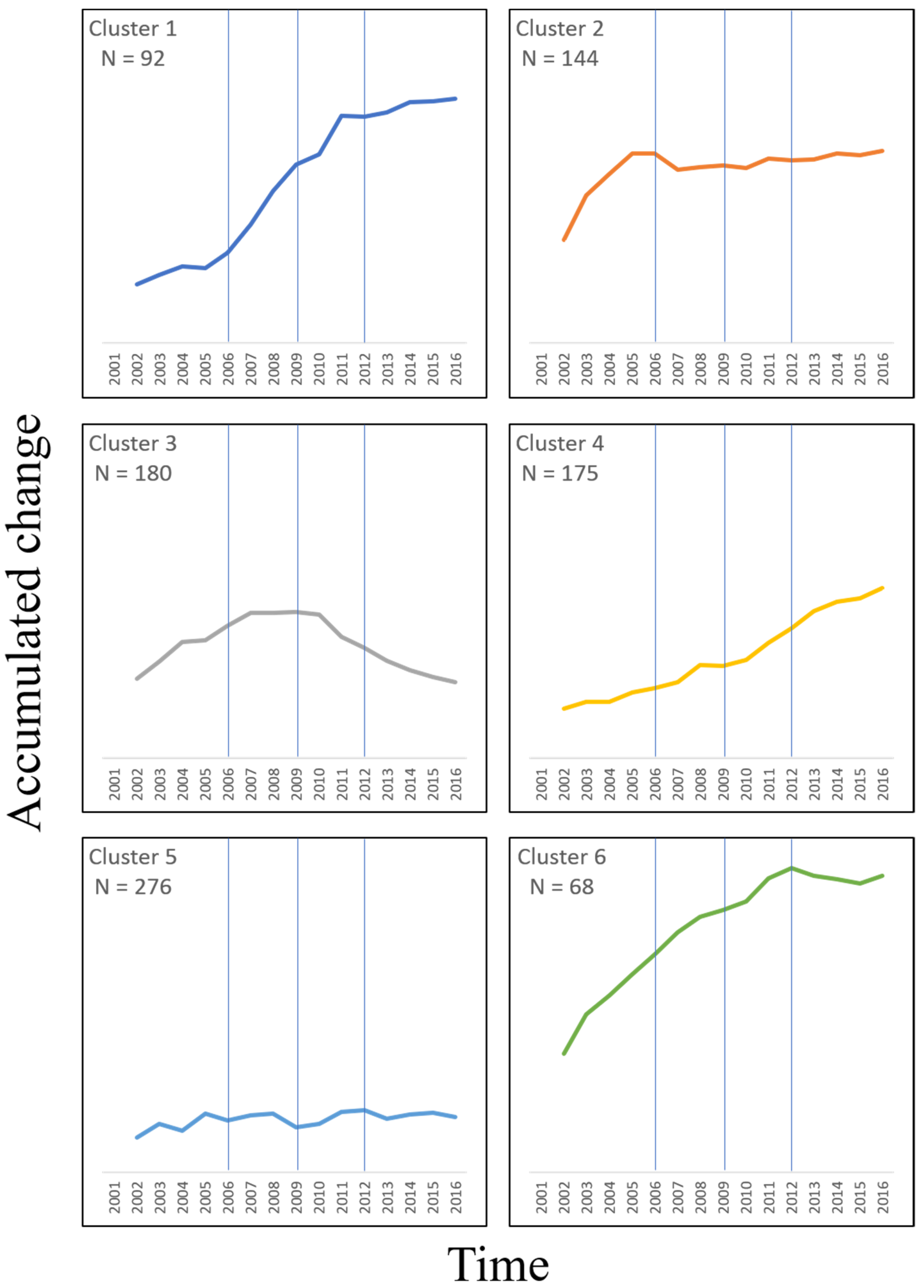
Our analysis identified six clusters of urban systems based on how their economic structures changed over time. For each of those clusters we plotted the average magnitude of accumulated system change over time (Figure 3). Qualitative descriptions of each archetype are presented in Table 1 along with each cluster’s average economic performance, measured as change in per capita GDP. GDP changes are presented for the recession period (2006–2009), the recovery period (2009–2012), and for the full period of the shock, which we take to include the recession and recovery.
Every cluster experienced a decrease in per capita GDP from 2006–2009 followed by an increase, or rebound, in per capita GDP from 2009–2012. However, only in cluster 4 was the rebound in per capita GDP greater than the initial drop, resulting in a net increase in per capita GDP of 1.4% over the full period of the recession.
Cluster 1 showed both the greatest decrease in per capita GDP during the initial recession (−7.5%) and the greatest gain during the recovery (+5.3%), but still had a net negative change in per capita GDP over the full period of the shock.
We note that the archetypical curve for Cluster 3 most closely corresponds to the classic notion of resilience in Figure 1c, yet this cluster had the worst economic performance of any cluster across the full shock period, exhibiting a net decline in per capita GDP of 2.7% from 2006–2012. On the other hand, Cluster 1, which best corresponds to a flip to a new stable state, as in Figure 1d, did not perform much better than did Cluster 3, having a 2.2% decrease in per capita GDP over the same period.
Cluster 5, which represents cities that exhibited virtually no change before, during, or after the shock, also experienced a negative overall change in performance. We take this as an indication that, while cities in Cluster 5 may have changed little, the environment in which they are embedded did change. As the authors of [50] state, “even an unperturbed system is not stable if the context changes around it.”
4. Discussion
4.1. Resilience of the System versus Resilience of Some System Output
Our findings highlight an area of obstinate confusion in the resilience dialog. Often it is not the return of the system to some previous state that is called resilience, but the return of some (often desirable) attribute of that system to its previous level that is called resilience. In this study, we take per capita GDP is to be a desirable attribute of an urban economy [8,28] and find that its return to a previous level following a shock was generally accompanied by substantial change in the system’s holistic structure. Thus, while an important system attribute may return to a previous level, the system’s overall structure rarely does.
More importantly our findings support the notion that conceptualizations of system response, such as those shown in Figure 1a,b, are naïve because the exogenous environment or fitness landscape in which they are embedded is characterized as unchanging (or at least dynamically stable over long periods of time). Instead, we find for urban economies that the conceptualization of “adaptive resilience” visualized by Laboy and Fannon [50] in Figure 4 best describes our results.
Thus, as a system changes in response to a shock, the system’s exogenous environment also changes, so that the concept of returning to a previous state loses much of its meaning. It is likely that such shifting stability domains are frequent in real-world complex adaptive systems and that systems and their environments co-evolve with one another in an endless dance of evolutionary dynamics. This view concurs with an emerging perspective in which the concept of economic equilibrium is largely rejected [51] and economics is instead framed as an evolutionary science [52].
Such a perspective is to be expected, for if we are concerned with the resilience of a complex adaptive system, then it follows that our system of interest must be adapting to something. That something is the system’s exogenous environment and it further follows that it is the changes in that external environment that create the impetus for our system of interest to adapt. Thus, it is likely that the resilience of most, if not all, complex adaptive systems is best described by the shifting stability domain of [50].
This view of a dynamic environment may explain why archetype 4—the only cluster with a net positive change in per capita GDP—was also the only archetype that continued to increase accumulated change after the shock. We characterize cluster 4 as exhibiting slow and steady change before, during, and after the shock. This suggests that systems that are dynamic and undergoing continuous and measured change better embody the idea of adaptation than systems exhibiting a large capacity for absorbing a shock, such as those represented in Figure 1c.
The results of this study have significant implications for policy makers concerned with managing for resilience. Our findings suggest that policy makers essentially face a moving target and that agility and adaptability are perhaps more important management objectives than specific targets of resilience.
4.2. Future Directions
This study operationalizes urban economic structures based on interdependencies between economic activities. Yet, those urban units are themselves interdependent with other cities, both nationally and internationally, through such links as product flows, financial links, trade agreements, and information sharing [53,54,55]. In other words, the networks representing cities in our study are themselves embedded in city–city networks of interdependence. Future studies should seek to couple our economic structures with these city–city networks to further refine measures of local vulnerability. Such models may allow researchers to better anticipate local impacts of global or far away disruptions, such as trade wars or distant environmental shocks [56].
Furthermore, while we used interdependencies between industries to create networks of urban economies, the methodology could be generalized to, for example, use interdependencies between skills or occupations to create networks of industries. Following the structure of this study, researchers might then be able to suggest a typology of industries based on how their structures respond to shocks as well as simply which industries are undergoing rapid reconfigurations relative to other industries.
Finally, it is important to note that resilience need not be a desirable system attribute. There are highly resilient, undesirable systems, such as degraded grasslands or feudal social systems, that last centuries. Thus, in any social system, in addition to assessing resilience, it is worthwhile to ask whether new states (accessed through a loss of resilience relative to the original state) are better or worse than the original state. One must also recognize that in social systems, rapid and substantial change—even if the end state is more desirable—is often accompanied by significant human suffering as social support systems strain to address transition impacts. This study shows that urban economies undergoing steady, but incremental, change prior to a large disturbance not only were more resilient but were the only type to exhibit increased productivity (higher per capita GDP) over the entire period of the recession and recovery. Future studies should examine households in each of our urban typologies to assess fine scale details of human advancement or suffering during the recession—whether a more resilient and desirable state at the level of the CBSA translates to more desirable outcomes at lower levels of organization.
Author Contributions
Conceptualization, S.T.S.; Data curation, S.T.S.; Funding acquisition, S.T.S.; Investigation, S.T.S., S.S.K., and F.W.; Methodology, S.T.S., S.S.K., and F.W.; Writing—original draft, S.T.S., S.S.K., F.W., and A.P.K.; Writing—review and editing, S.T.S., S.S.K., F.W., and A.P.K. All authors have read and agreed to the published version of the manuscript.
Funding
The authors received funding from the ASU Knowledge Exchange for Resilience. The ASU Knowledge Exchange for Resilience is supported by Virginia G. Piper Charitable Trust. Piper Trust supports organizations that enrich health, well-being, and opportunity for the people of Maricopa County, Arizona. The conclusions, views and opinions expressed in this article are those of the authors and do not necessarily reflect the official policy or position of the Virginia G. Piper Charitable Trust.
Institutional Review Board Statement
Not applicable.
Informed Consent Statement
Not applicable.
Data Availability Statement
All data used in this study are publicly available as described in the paper.
Acknowledgments
The authors thank Dylan Weber for assistance with the Python/R coding.
Conflicts of Interest
The authors declare no conflict of interest. The funders had no role in the design of the study; in the collection, analyses, or interpretation of data; in the writing of the manuscript, or in the decision to publish the results.
References
- Loorbach, D.; Wittmayer, J.M.; Shiroyama, H.; Fujino, J.; Mizuguchi, S. (Eds.) Governance of Urban Sustainability Transitions; Springer: Tokyo, Japan, 2016. [CrossRef]
- Yanarella, E.J.; Levine, R.S. The City as Fulcrum of Global Sustainability; Anthem Press: London, UK, 2011. [Google Scholar]
- Li, Q. Resilience Thinking as a System Approach to Promote China’s Sustainability Transitions. Sustainability 2020, 12, 5008. [Google Scholar] [CrossRef]
- Schilling, T.; Wyss, R.; Binder, C.R. The Resilience of Sustainability Transitions. Sustainability 2018, 10, 4593. [Google Scholar] [CrossRef] [Green Version]
- Scheffer, M.; Carpenter, S.; Foley, J.A.; Folke, C.; Walker, B. Catastrophic shifts in ecosystems. Nature 2001, 413, 591–596. [Google Scholar] [CrossRef] [PubMed]
- Romero-Lankao, P.; Gnatz, D.M.; Wilhelmi, O.; Hayden, M. Urban Sustainability and Resilience: From Theory to Practice. Sustainability 2016, 8, 1224. [Google Scholar] [CrossRef] [Green Version]
- Rose, A. Economic Resilience and Its Contribution to the Sustainability of Cities. In Resilience and Sustainability in Relation to Natural Disasters: A Challenge for Future Cities; Gasparini, P., Manfredi, G., Asprone, D., Eds.; Springer International Publishing: Cham, Switzerland, 2014; pp. 1–11. [Google Scholar] [CrossRef]
- United Nations General Assemby. Transforming our world: The 2030 Agenda for Sustainable Development; United Nations General Assembly: New York, NY, USA, 2015. [Google Scholar]
- Collier, M.J.; Nedović-Budić, Z.; Aerts, J.; Connop, S.; Foley, D.; Foley, K.; Newport, D.; McQuaid, S.; Slaev, A.; Verburg, P. Transitioning to resilience and sustainability in urban communities. Cities 2013, 32, S21–S28. [Google Scholar] [CrossRef] [Green Version]
- Moore, T.; Haan, F.D.; Gleeson, B.J. Urban Sustainability Transitions: An Emerging Hybrid Research Agenda. In Urban Sustainability Transitions; Frantzeskaki, N., Broto, V.C., Coenen, L., Loorbach, D., Eds.; Springer: Singapore, 2018; pp. 253–257. [Google Scholar] [CrossRef]
- Team, V.; Manderson, L. How COVID-19 Reveals Structures of Vulnerability. Med. Anthropol. 2020, 39, 671–674. [Google Scholar] [CrossRef] [PubMed]
- Mishra, S.V.; Gayen, A.; Haque, S.M. COVID-19 and urban vulnerability in India. Habitat Int. 2020, 103, 102230. [Google Scholar] [CrossRef]
- Shamasunder, S.; Holmes, S.M.; Goronga, T.; Carrasco, H.; Katz, E.; Frankfurter, R.; Keshavjee, S. COVID-19 reveals weak health systems by design: Why we must re-make global health in this historic moment. Glob. Public Health 2020, 15, 1083–1089. [Google Scholar] [CrossRef]
- Gaynor, T.S.; Wilson, M.E. Social Vulnerability and Equity: The Disproportionate Impact of COVID-19. Public Adm. Rev. 2020, 80, 832–838. [Google Scholar] [CrossRef]
- Shutters, S.T. Urban Science: Putting the “Smart” in Smart Cities. Urban Sci. 2018, 2, 94. [Google Scholar] [CrossRef] [Green Version]
- McHale, M.R.; Pickett, S.T.A.; Barbosa, O.; Bunn, D.N.; Cadenasso, M.L.; Childers, D.L.; Gartin, M.; Hess, G.R.; Iwaniec, D.M.; McPhearson, T.; et al. The New Global Urban Realm: Complex, Connected, Diffuse, and Diverse Social-Ecological Systems. Sustainability 2015, 7, 5211. [Google Scholar] [CrossRef] [Green Version]
- Gunderson, L.H.; Holling, C.S. (Eds.) Panarchy: Understanding Transformations in Human and Natural Systems; Island Press: Washington, DC, USA, 2002. [Google Scholar]
- Xu, L.; Marinova, D. Resilience thinking: A bibliometric analysis of socio-ecological research. Scientometrics 2013, 96, 911–927. [Google Scholar] [CrossRef] [Green Version]
- Shutters, S.T.; Waters, K. Inferring Networks of Interdependent Labor Skills to Illuminate Urban Economic Structure. Entropy 2020, 22, 1078. [Google Scholar] [CrossRef]
- Muneepeerakul, R.; Lobo, J.; Shutters, S.T.; Goméz-Liévano, A.; Qubbaj, M.R. Urban Economies and Occupation Space: Can They Get “There” from “Here”? PLoS ONE 2013, 8, e73676. [Google Scholar] [CrossRef] [Green Version]
- Janssen, M.A.; Bodin, Ö.; Anderies, J.M.; Elmqvist, T.; Ernstson, H.; McAllister, R.R.J.; Olsson, P.; Ryan, P. Toward a network perspective on the resilience of social-ecological systems. Ecol. Soc. 2006, 11, 15. [Google Scholar] [CrossRef] [Green Version]
- Han, Y.; Goetz, S.J. Predicting US county economic resilience from industry input-output accounts. Appl. Econ. 2019, 51, 2019–2028. [Google Scholar] [CrossRef]
- Shutters, S.T.; Muneepeerakul, R.; Lobo, J. Quantifying urban economic resilience through labour force interdependence. Palgrave Commun. 2015, 1, 1–7. [Google Scholar] [CrossRef] [Green Version]
- Berkes, F.; Colding, J.; Folke, C. (Eds.) Navigating Social-Ecological Systems: Building Resilience for Complexity and Change; Cambridge University Press: Cambridge, UK, 2002. [Google Scholar]
- Eason, T.; Garmestani, A. Cross-scale dynamics of a regional urban system through time. Reg. Dev. 2012, 36, 55–77. [Google Scholar]
- Levin, S.A. Fragile Dominion: Complexity and the Commons; Perseus Publishing: Cambridge, MA, USA, 1999. [Google Scholar]
- Ludwig, D.; Walker, B.; Holling, C.S. Sustainability, Stability, and Resilience. Ecol. Soc. 1997, 1, 7. [Google Scholar] [CrossRef]
- United Nations. New Urban Agenda; United Nations Habitat III Secretariat: Quito, Ecuador, 2017.
- Hidalgo, C.A.; Klinger, B.; Barabasi, A.L.; Hausmann, R. The product space conditions the development of nations. Science 2007, 317, 482–487. [Google Scholar] [CrossRef] [Green Version]
- Frenken, K.; Van Oort, F.; Verburg, T. Related Variety, Unrelated Variety and Regional Economic Growth. Reg. Stud. 2007, 41, 685–697. [Google Scholar] [CrossRef] [Green Version]
- Essletzbichler, J. Relatedness, Industrial Branching and Technological Cohesion in US Metropolitan Areas. Reg. Stud. 2015, 49, 752–766. [Google Scholar] [CrossRef] [Green Version]
- Alabdulkareem, A.; Frank, M.R.; Sun, L.; AlShebli, B.; Hidalgo, C.; Rahwan, I. Unpacking the polarization of workplace skills. Sci. Adv. 2018, 4, eaao6030. [Google Scholar] [CrossRef] [Green Version]
- Neffke, F.; Henning, M.; Boschma, R. How Do Regions Diversify over Time? Industry Relatedness and the Development of New Growth Paths in Regions. Econ. Geogr. 2011, 87, 237–265. [Google Scholar] [CrossRef]
- O’Clery, N.; Heroy, S.; Hulot, F.; Beguerisse-Diaz, M. Unravelling the forces underlying urban industrial agglomeration. arXiv 2019, arXiv:1903.09279v2. [Google Scholar]
- Jara-Figueroa, C.; Jun, B.; Glaeser, E.L.; Hidalgo, C.A. The role of industry-specific, occupation-specific, and location-specific knowledge in the growth and survival of new firms. Proc. Natl. Acad. Sci. USA 2018, 115, 12646. [Google Scholar] [CrossRef] [Green Version]
- Shutters, S.T.; Lobo, J.; Strumsky, D.; Muneepeerakul, R.; Mellander, C.; Brachert, M.; Fernandes, T.F.; Bettencourt, L.M.A. The relationship between density and scale in information networks: The case of urban occupational networks. PLoS ONE 2018, 15, e0196915. [Google Scholar] [CrossRef] [Green Version]
- Farinha, T.; Balland, P.-A.; Morrison, A.; Boschma, R. What drives the geography of jobs in the US? Unpacking relatedness. Ind. Innov. 2019, 26, 988–1022. [Google Scholar] [CrossRef] [Green Version]
- Kok, S.; Weel, B.T. Cities, tasks, and skills. J. Reg. Sci 2014, 54, 856–892. [Google Scholar] [CrossRef]
- Boschma, R.; Balland, P.-A.; Kogler, D.F. Relatedness and technological change in cities: The rise and fall of technological knowledge in US metropolitan areas from 1981 to 2010. Ind. Corp. Chang. 2015, 24, 223–250. [Google Scholar] [CrossRef]
- U.S. Office of Management and Budget. OMB Bulletin No. 20-01: Revised Delineations of Metropolitan Statistical Areas, Micropolitan Statistical Areas, and Combined Statistical Areas, and Guidance on Uses of the Delineations of These Areas; U.S. Office of Management and Budget: Washington, DC, USA, 2020.
- U.S. Bureau of Labor Statistics. Quarterly Census of Employment and Wages. Available online: https://www.bls.gov/cew/ (accessed on 13 January 2020).
- U.S. Census Bureau. Delineation Files: Core Based Statistical Areas (CBSAs), Metropolitan Divisions, and Combined Statistical Areas (CSAs) (Version Sep. 2018). Available online: https://www.census.gov/geographies/reference-files/time-series/demo/metro-micro/delineation-files.html (accessed on 3 February 2020).
- U.S. Bureau of Economic Analysis. GDP by County, Metro, and Other Areas, Washington, DC, 2019. Available online: https://www.bea.gov/data/gdp/gdp-county-metro-and-other-areas (accessed on 17 January 2020).
- Schieber, T.A.; Carpi, L.; Díaz-Guilera, A.; Pardalos, P.M.; Masoller, C.; Ravetti, M.G. Quantification of network structural dissimilarities. Nat. Commun. 2017, 8, 13928. [Google Scholar] [CrossRef] [PubMed] [Green Version]
- Hamming, R.W. Error detecting and error correcting codes. Bell Syst. Tech. J. 1950, 29, 147–160. [Google Scholar] [CrossRef]
- Norouzi, M.; Fleet, D.J.; Salakhutdinov, R. Hamming distance metric learning. In Proceedings of the 25th International Conference on Neural Information Processing Systems—Volume 1, Lake Tahoe, NV, USA, 3–6 December 2012; pp. 1061–1069.
- Sanfeliu, A.; Fu, K. A distance measure between attributed relational graphs for pattern recognition. IEEE Trans. Syst. Man Cybern. 1983, SMC-13, 353–362. [Google Scholar] [CrossRef]
- Thorndike, R.L. Who belongs in the family? Psychometrika 1953, 18, 267–276. [Google Scholar] [CrossRef]
- Kaufman, L.; Rousseeuw, P.J. Finding Groups in Data: An Introduction to Cluster Analysis; John Wiley & Sons: Hoboken, NJ, USA, 2005. [Google Scholar]
- Laboy, M.; Fannon, D. Resilience Theory and Praxis: A Critical Framework for Architecture. Enquiry 2016, 13. [Google Scholar] [CrossRef] [Green Version]
- Evenhuis, E. New directions in researching regional economic resilience and adaptation. Geogr. Compass 2017, 11, e12333. [Google Scholar] [CrossRef]
- Ferreira, V. Why Economics Must be an Evolutionary Science; ISEG—Lisbon School of Economics and Management, Department of Economics, Universidade de Lisboa: Lisboa, Portugal, 2019. [Google Scholar]
- Qubbaj, M.R.; Shutters, S.; Muneepeerakul, R. Living in a Network of Scaling Cities and Finite Resources. Bull. Math. Biol. 2014, 77, 390–407. [Google Scholar] [CrossRef] [PubMed]
- Derudder, B.; Witlox, F. World City Networks and Global Commodity Chains: An introduction. Glob. Netw. 2010, 10, 1–11. [Google Scholar] [CrossRef] [Green Version]
- Khanna, P. Connectography: Mapping the Future of Global Civilization; Random House: New York, NY, USA, 2016. [Google Scholar]
- Sternberg, T. Chinese drought, bread and the Arab Spring. Appl. Geogr. 2012, 34, 519–524. [Google Scholar] [CrossRef]
Figure 1.
Conceptualizations of systems responding to a disturbance. The left panels demonstrate two possible trajectories of a system (the ball) following a disturbance. In the left panels the y-axis is an abstract and dimensionless representation of the system environment. In (a) the system moves away from its initial state and eventually returns. In (b) the system is disturbed sufficiently that it moves to a new stable state. Each diagram on the left can be transformed into a plot of accumulated change versus time as in (c) and (d). We created analogous diagrams using empirical data for 938 U.S. urban areas.

Figure 2.
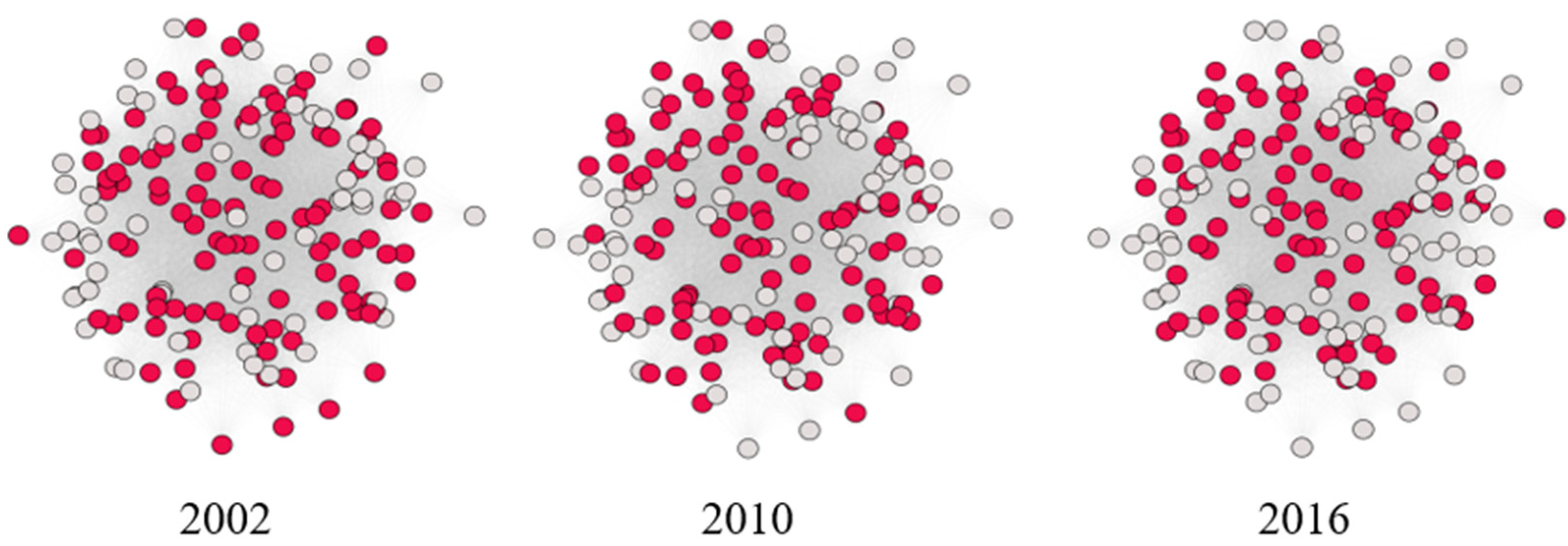
The industry structures of an example area, the Phoenix metropolitan statistical area, at three points in time. Highlighted nodes indicate industries that are present in a given year. Empty nodes are industries that exist elsewhere in the U.S. but are not present in Phoenix. Note that which industries are present change subtly over time as does the total number of industries present. We quantified the difference between these networks and took it as a measure of structural change over time.
Figure 2.
The industry structures of an example area, the Phoenix metropolitan statistical area, at three points in time. Highlighted nodes indicate industries that are present in a given year. Empty nodes are industries that exist elsewhere in the U.S. but are not present in Phoenix. Note that which industries are present change subtly over time as does the total number of industries present. We quantified the difference between these networks and took it as a measure of structural change over time.

Figure 3.
Average accumulated change by year among all cities of each cluster. Vertical bars in each panel represent, from left to right, beginning of recession (2006), end of recession/beginning of recovery (2009), and end of recovery (2012). The number of core based statistical areas (CBSAs) included in each cluster is shown under the cluster number. We take these curves to be the response archetypes of each cluster. Note that accumulated change is a dimensionless value and is always positive.

Figure 4.
While simplistic conceptualizations of system stability assume a fixed exogenous environment (left and center), urban economies are embedded in an environment that is itself dynamic and co-evolving (right). Figure courtesy of Laboy and Fannon [50].
Figure 4.
While simplistic conceptualizations of system stability assume a fixed exogenous environment (left and center), urban economies are embedded in an environment that is itself dynamic and co-evolving (right). Figure courtesy of Laboy and Fannon [50].


Table 1.
Comparison of average economic performance and other attributes of each cluster.
| Cluster Archetype | Description | Mean 2006 Population (Thousands) | Change in Per Capita GDP 2006–2009 | Change in Per Capita GDP 2009–2012 | Net Change in Per Capita GDP |
|---|---|---|---|---|---|
 | Stable systems that changed rapidly during recession then became stable at a new position. Similar to the classical notion of a system flipping to a new stable state. | 244 | −7.5% | +5.3% | −2.2% |
 | Systems that underwent rapid change until the recession and then stopped changing for the duration of the study period, well beyond the recession. | 952 | −4.6% | +3.7% | −0.9% |
 | Systems that changed in response to the recession but then returned to their previous state after the recession. Similar to the classical notion of a resilient system. | 187 | −5.2% | +2.5% | −2.7% |
 | Systems that underwent slow but steady change before, during, and after the recession, seemingly unaffected by the recession. | 140 | −1.0% | +2.4% | +1.4% |
 | Systems seemingly unchanged during the entire study period, including in response to the recession. | 74 | −4.1% | +2.6% | −1.5% |
 | Systems that underwent rapid change before the recession, continued rapid change during the recession, but then stopped changing after recovery. | 600 | −4.3% | +1.1% | −2.2% |
Publisher’s Note: MDPI stays neutral with regard to jurisdictional claims in published maps and institutional affiliations. |
© 2021 by the authors. Licensee MDPI, Basel, Switzerland. This article is an open access article distributed under the terms and conditions of the Creative Commons Attribution (CC BY) license (http://creativecommons.org/licenses/by/4.0/).
Share and Cite
MDPI and ACS Style
Shutters, S.T.; Kandala, S.S.; Wei, F.; Kinzig, A.P. Resilience of Urban Economic Structures Following the Great Recession. Sustainability 2021, 13, 2374. https://0-doi-org.brum.beds.ac.uk/10.3390/su13042374
AMA Style
Shutters ST, Kandala SS, Wei F, Kinzig AP. Resilience of Urban Economic Structures Following the Great Recession. Sustainability. 2021; 13(4):2374. https://0-doi-org.brum.beds.ac.uk/10.3390/su13042374
Chicago/Turabian StyleShutters, Shade T., Srinivasa S. Kandala, Fangwu Wei, and Ann P. Kinzig. 2021. "Resilience of Urban Economic Structures Following the Great Recession" Sustainability 13, no. 4: 2374. https://0-doi-org.brum.beds.ac.uk/10.3390/su13042374
Note that from the first issue of 2016, this journal uses article numbers instead of page numbers. See further details here.