1. Introduction
The United Nations predict that 9.7 billion people will live in cities by 2050 [
1]. Along with the effects of climate change, cities face numerous challenges as their resources and infrastructure are placed under ever increasing levels of strain [
2]. As water scarcity becomes more prevalent, the analysis of urban water consumption patterns for consumers and the estimation of the corresponding water demand are expected to be among the top priorities for water companies in the near future. There is a constant need to improve the knowledge of urban water demand and of factors that influence demand patterns in a household; this requires collection and analysis of water consumption data, which can be facilitated by Information and Communication Technology (ICT) systems in a smart city framework. ICTs can help managers in integrating the water sector with other city services and in monitoring their status in real time. This results in several operational benefits that optimize urban water management, including real time demand forecasting and optimization of network devices and of operating costs [
3]. On this basis, it is possible to develop better water demand models and new customer-oriented tools to be used for smart metering, smart pricing and tariff planning, water distribution network planning and operation, energy savings in water transfer, and customer service and billing, as well as the real-time management of condition-based tariffs. These goals abide by the European legislation, as described in the EU Water Framework Directive and the Blueprint to safeguard Europe’s water resources [
4] concerning water accounts and ecological flows, water pricing, water trading, and other factors. Furthermore, the recent technological progress in wireless sensors that enable monitoring of water use in individual households, or even in different faucets or appliances inside a single household, can provide detailed information concerning spatial and temporal water use patterns. These data have been collected in the past mainly for research purposes [
5,
6,
7] but are now becoming more common with the diffusion of smart city initiatives, such as the installation of smart water meters [
8]. In the future, the availability of such information will allow for more accurate billing and customer-specific services, but, more importantly, will increase water efficiency due to a better understanding of the water consumption behavior at household levels for both large and small customers and may help in the reduction of non-revenue water.
In order to assess urban water demand in time and space, a water consumption profile curve is needed. This curve shows the amount of water a customer uses over the course of time and it is useful for planning how much water the utility will need to make available for its customers at any given time. Furthermore, water consumption profiles reveal the pattern customers exhibit in using water at different hours of the day, days of the week and seasons of the year, and can specify what the customer’s share of the utility’s total water consumption is. By analogy with electricity load curves, water consumption profiles can provide estimates of the temporal and spatial distribution of demand, thus giving insight into peak demands at different locations [
9]. The major factors affecting the consumption profile are (1) family size and customer water use behavior, as well as residence characteristics and (2) seasonality, i.e., time of day, week, or year. Local climate factors such as temperature, humidity, and solar radiation may play an important role in water consumption patterns, but their effect is captured by seasonality [
10].
Even though it is typical for energy and telecommunication companies to classify their customers into groups with similar consumption patterns taking into account their characteristics and annual demand, such practices are not common for water utilities, maybe because of the relatively low cost of water. The goal of this classification is to assign to each customer a variable estimate of consumption, a sort of a “load curve”, in the absence of available meter data. These pre-fixed curves may also be useful for market investigation and distribution management for the utility. Yet, they have flaws as a result of their coarseness, since on the one hand, they may fail to follow actual consumptions, and on the other, they are unable to predict possible changes in people’s way of life and/or in their consumption patterns [
11]. It is undisputed that a more thorough description and forecast of water consumption throughout the day, month, and year, capturing seasonality and weekday/weekend patterns in water use can lead to an improved management and planning of demand and distribution, resulting in a potential reduction of costs for the water utility. Understanding customer behavior can lead to a successful categorization based on the recognition of similarities in consumption patterns among consumers. This segmentation would allow water utilities to better tailor pumping, treatment, and network operation, while it can provide useful information on water pricing policies and other incentive-creation strategies [
12].
Many researchers have shown an increasing interest in Artificial Neural Networks (ANN) to address various kinds of problems in water resources and hydrology [
13,
14,
15,
16]. Self-Organizing Maps (SOMs) is an ANN algorithm [
17,
18], which has proven to be an excellent tool for clustering, classification, estimation, prediction, and data mining [
19,
20,
21]. Kalteh et al. [
22] reviewed a number of successful SOM applications with emphasis on innovative and creative solutions for the analysis, estimation, and prediction of various hydrological processes, such as precipitation [
23,
24,
25], river flow and rainfall-runoff [
26,
27,
28], surface water quality [
29,
30,
31,
32], and other related disciplines such as climate and environment [
33,
34,
35]. SOMs have many applications in signal recognition, organization of large data sets, process monitoring and analysis, and over the last decades, they have increasingly been used for analysis and modeling in the energy domain [
9,
36,
37,
38]. However, only a limited number of articles have been published on domestic water consumption pattern recognition, classifying customers in different segments [
39,
40,
41].
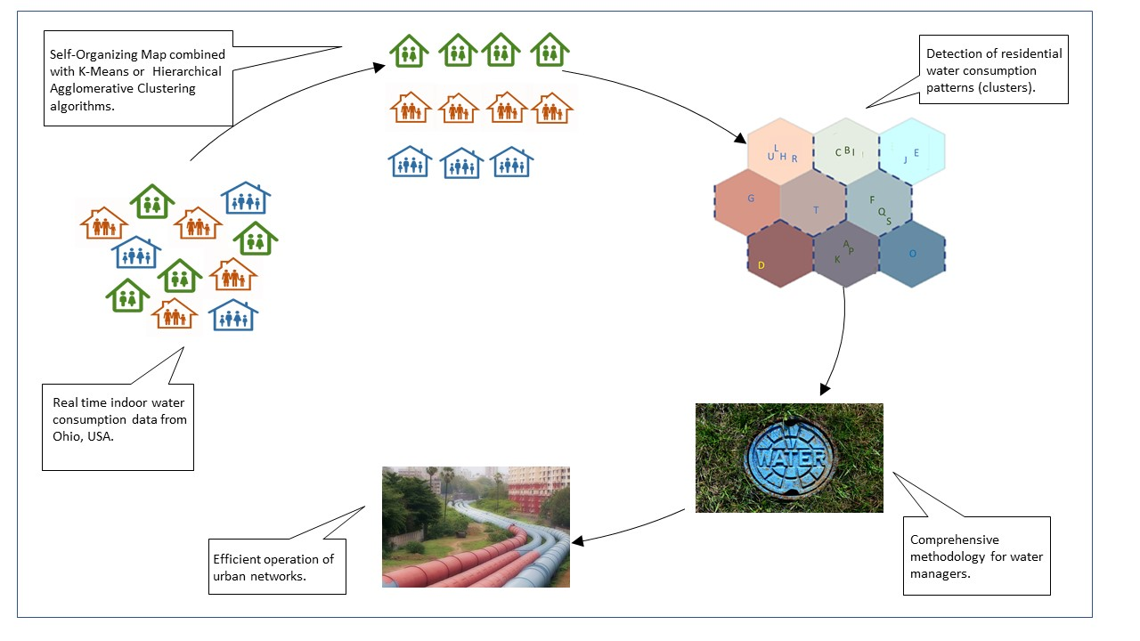
This study aims to bridge this gap by proposing a comprehensive methodology to residents, water managers, and policy makers, in order to achieve the efficient operation of urban water networks by successfully detecting residential water consumption patterns corresponding to different residential needs and behaviors. This way, households with similar consumption patterns are grouped in clusters. A large dataset taken from the work of Buchberger et al. [
42] and consisting of 7 months of water consumption data recording every instant of water use in the household from 21 customers located in Milford, Ohio, USA, was examined. To the best of the authors’ knowledge, residential water consumption data with this granularity have not been analyzed for the purpose of detecting behavioral patterns in water consumption. The aim of the article is to create more accurate customer-specific water consumption curves using refined measurement data. In this context, we propose a methodology that may be applied in complex and large water consumption time-series, using SOMs as the main clustering algorithm, in combination with K-Means (KM) and Hierarchical Agglomerative Clustering (HAC) to improve performance; this way, we provide a new-estimated water consumption profile for each customer group. The resulting curves that are obtained after clustering customers with similar consumption behavior are compared to the water consumption curves that the water company might use to create timely customer water use estimates without performing clustering. The results indicate that there is a clear improvement when using the newly estimated, data-based water consumption curves after clustering. This analysis offers water utilities an innovative solution that relies on real time data and uses data science principles relevant to a smart city setting for optimizing water supply and network operation and leading to efficient resource use. It creates opportunities to engage citizens while raising their awareness of household water consumption. Therefore, it lays the foundation for developing behavioral change processes for citizens towards more sustainable water use patterns that would reduce their environmental footprint, change their consumption and lifestyle choices, and achieve a climate-neutral way of living.
2. Materials and Methods
In order to develop reliable water consumption curves for customers belonging to different classes, large numbers of recorded water consumption values are required—for electricity, it is recommended to have at least 100 customers over a period of 3 years [
43]. For household water consumption, such long datasets are unavailable due to the very recent implementation of smart technologies in the water sector, which is often confined to limited duration of research projects e.g., Yang et al. [
7]. In this article, we use the data collected by Buchberger et al. [
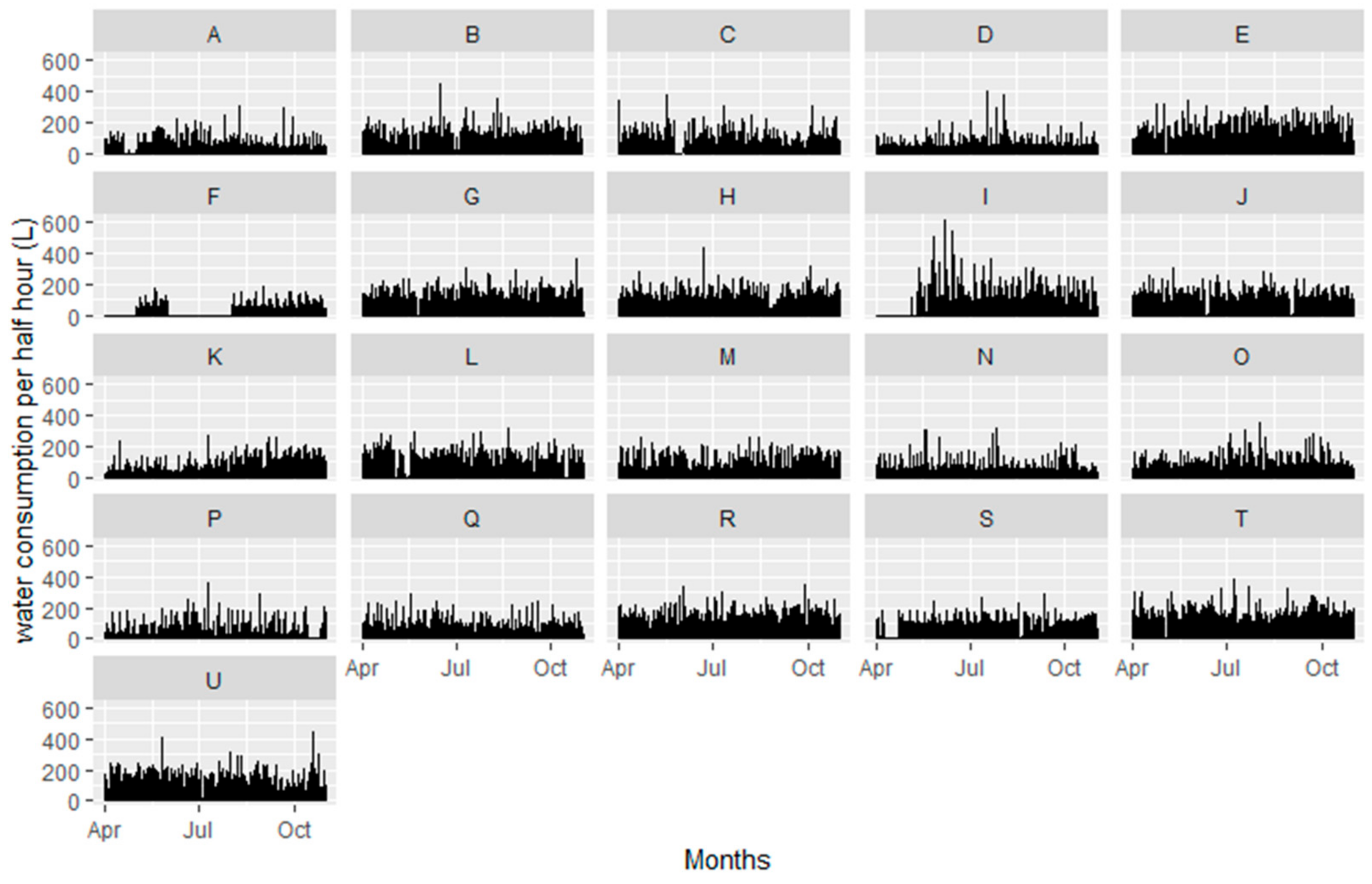
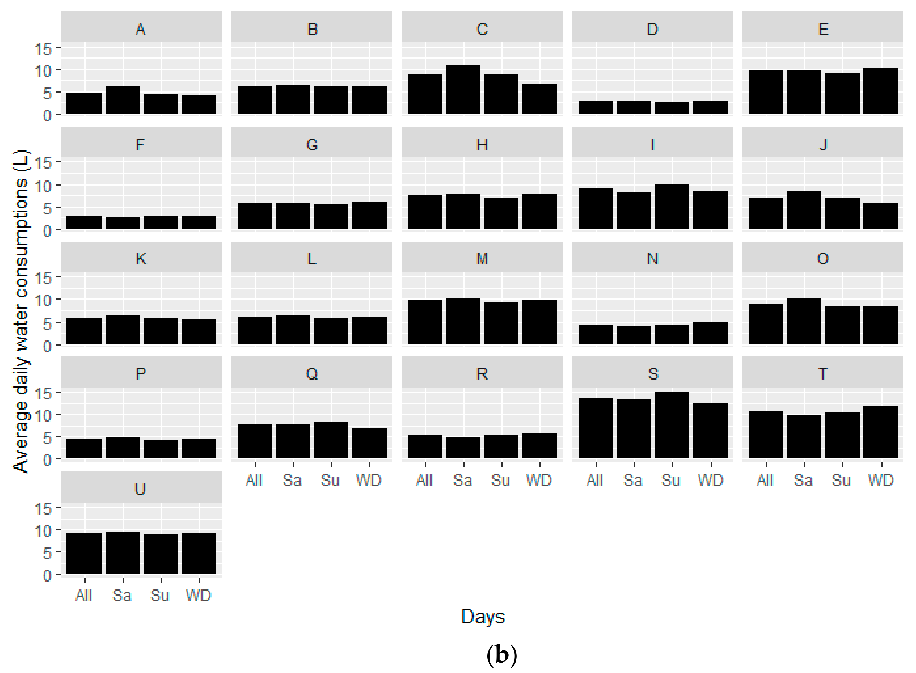
42], who carried out an experimental campaign aimed at monitoring residential water demand in the period from April to October 1997 in 21 households in Milford, OH, USA. An electromagnetic flowmeter was installed in the mainline of each household and water discharge data was collected for the 7-month period with a resolution of 1 s. It should be noted here that only indoor water consumption was included in our data, so even if a household had large gardens, or a swimming pool, it would not make a difference to our dataset. To create a uniform time series for all households, we grouped all water consumption data (210 days) to half-hour slots, resulting in a dataset of 10,080 entries for each household. In
Figure 1, we show graphs of the consumption dataset for all households—each bar corresponds to the half-hour consumption and there are a total of 10,080 bars in each graph. To show the variation of consumption over weekdays and weekends, in
Figure 2a, we show, indicatively for household C, average consumptions of all weekday, Saturday, and Sunday consumptions per half-hour time slot throughout the day, for a total of 48 time slots per day. This provides more information on the consumption pattern of each household. In
Figure 2b, we show for each household, the average total daily consumption for all days and for weekdays, Saturdays, and Sundays. We notice that all households show high average daily water consumptions ranging from 229 liters/day (household F) to 875 liters/day (household T). It should be noted that the low average of household F is a result of many days with zero consumption. 19 households were used for the application of the clustering algorithm, simulating the procedure that the water utility would follow for clustering existing customers; on the other hand, two households, namely households M and N, were set aside and were assigned to clusters later, in order to simulate how well new customers would fit in pre-existing clusters. The number of households that was set aside was kept to a minimum (9.5% of the total data), since a very limited number of households is available in our dataset. Other researchers that have conducted similar analysis with electricity data, e.g., Rasanen et al. [
9], used 5.6% of their data to simulate “new customers”, so for our case, the small number of data reserved for validation is deemed acceptable.
2.1. Clustering Methods
SOMs are well-known unsupervised neural learning algorithms [
44] and an effective software tool for the modeling and visualization of high-dimensional data. They use unsupervised learning to group input data and produce a low-dimension discretized representation of the input space, i.e., a map. An SOM uses specific features of a population, such as household surface area, income level, age, number of bathrooms, etc. It calculates the Euclidean distance of each population unit, taking into account the features as dimensions or components of the input vectors. It then converts the multidimensional positions of the units into a 2-dimensional space and maps them. These maps (SOMs) depict all units as points in space in a sense that neighboring points have similar features; this way, clustering of similar units is made possible. In this work, an SOMs algorithm was applied as an intermediate step before the clustering process since it reduces the size of the data and makes the computational procedure more efficient. A feature-extraction approach was used to explore the data set and to identify which consumer properties are relevant to be included by the water utility in an automatic classification system [
45]. In
Table 1, we list the features that were chosen: they include a statistical property of the dataset (standard deviation) and are based on consumption values of individual days, as well as aggregated over the entire week, over workdays and weekends separately and over seasons. Since our benchmark dataset runs from April to October, we considered separately water use during the summer (June, July, and August) and autumn months (September and October). We used SOMs to calculate the Euclidean distance of the data and to find which households are in the same “neighborhood” or belong to the same cluster. This way, a map emerged consisting of nodes or neurons–in our case, various map sizes were tried, and the 3 × 3 size map was chosen with 9 nodes, since this number of nodes achieved the highest SOM’s clustering efficiency (95%). The lattice of the SOM can be either hexagonal or rectangular but hexagonal is preferred for this methodology due to more effective visualization [
21,
46]. All data were automatically normalized by the SOMs algorithm on a scale 0 to 1. All calculations were performed with RStudio [
47], using the “Kohonen” package.
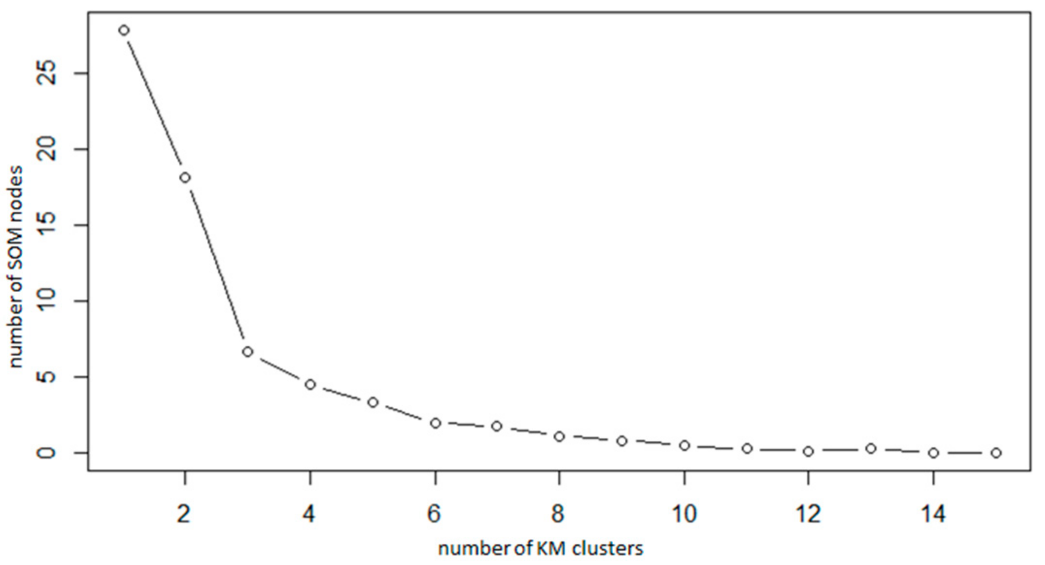
Once the SOMs algorithm is run and the map is obtained, it can be followed by a second step in which it is combined with other clustering algorithms. The main advantage of using this two-step approach is improved clustering. More specifically, while the SOMs algorithm provides a map of 9 nodes, its combination with other procedures results in fewer clusters (collecting various nodes in larger clusters) with higher accuracy. For this purpose, SOMs were combined with two other clustering algorithms: (1) K-Means clustering (KM) and (2) Hierarchical Agglomerative Clustering (HAC). KM [
48] is a well-known non-hierarchical clustering algorithm with many applications in different domains. The exact number of clusters was decided by calculating the Within-Clusters-Sum-of-Squares (WCSS) measurement that denotes the total distance of data points from their respective cluster centroids [
49]. Considering that we have nine SOM nodes, the ideal number of clusters proposed by KM is three, since this number is the closest match to the corresponding number of SOM nodes, when WCSS is calculated, as shown in
Figure 3.
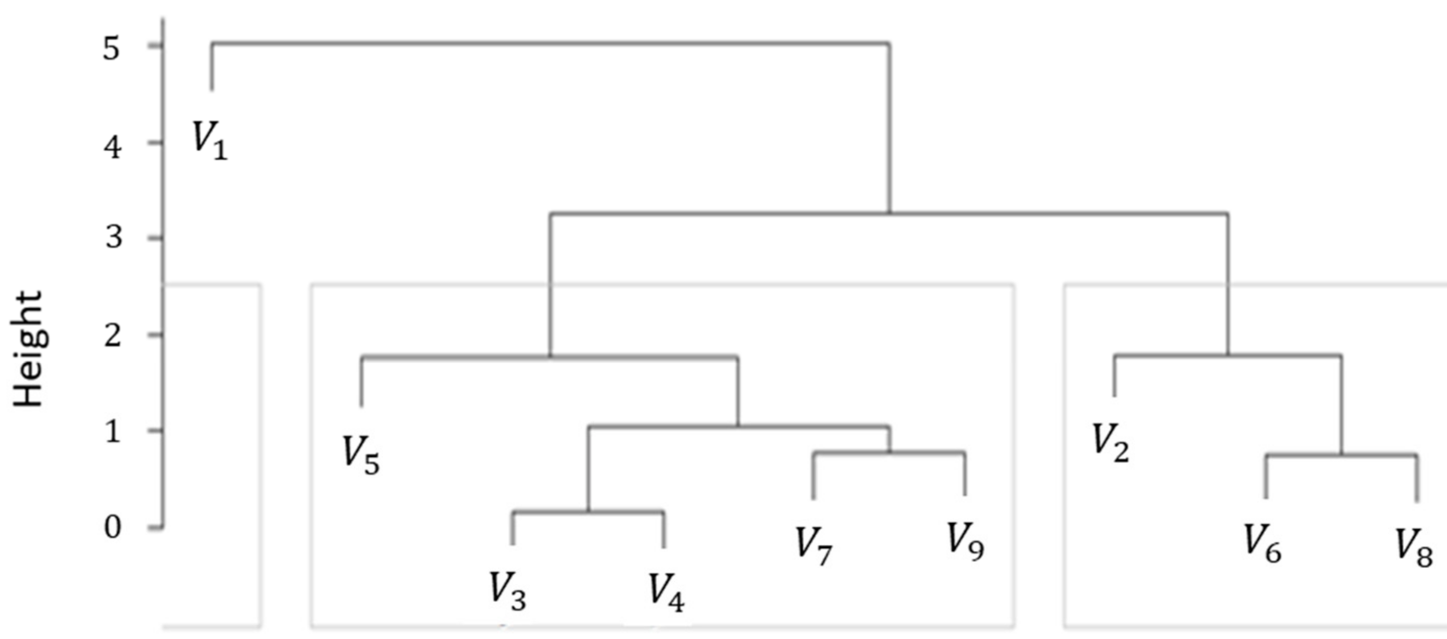
HAC is another popular clustering algorithm [
50]. It creates a cluster dendrogram (tree) by grouping several data together over a variety of scales and based on this classification, a clustering scheme emerges. Three clusters were formed from the HAC tree map with this analysis, as shown in
Figure 4 in grey boxes, which group different SOM nodes, or codebook vectors (shown as V1 to V9). Even though the number of clusters is the same with the two algorithms, the specific SOM nodes grouped under each clustering methodology are different, essentially each one providing a different clustering solution that is separately evaluated for its accuracy.
In order to assess the clustering accuracy, we want to know if the features we extracted on water consumption (
Table 1), actually force households to group together under the same cluster. Ideally, we would use a series of known properties about our households to identify the ones that are particularly relevant, as far as the domestic water consumption pattern is concerned. Examples include size of house and year built, garden and/or swimming pool, number and age of residents, number of appliances/washers, etc. We would then see which of these properties vary significantly among clusters or can likely be discovered from the data. If a property seems to vary across clusters, it will mean that it is a good property to group households by, and that using the set of features we defined in
Table 1, it is possible to differentiate households by that specific property. In our case, the only household property available for the 21 customers is the number of people per residence; this information is shown in
Table 2. Naturally, this is a serious limitation in our data set; however, all households came from the same neighborhood in suburban Ohio, so we expect that the houses have some similarities in terms of year built, surface area, amenities, etc. Nevertheless, our only choice is to use number of residents per household to check whether it is appropriate to group households according to it and to calculate clustering accuracy based on this property. We do this only after we confirm that indeed this property varies across clusters, as explained above. Based on the calculation of this accuracy, we decide on the best combined clustering algorithm (SOM+KM or SOM+HAC) and on the final clustering of the households.
2.2. Validation: Estimated Water Consumption Curves and Associated Accuracy
After clustering, the new estimated water consumption curves are calculated for each cluster. These are the curves that would be used by the water utility for all customers belonging in the same cluster, in order to successfully estimate the next customer bill, or plan for the estimated water demand in the network. For comparison purposes, we calculate two types of estimated curves: one for each cluster and one for all households if no prior clustering is performed. The goal is to show that clustering improves estimated water consumption, namely that the index of agreement of customer consumption with the estimated water consumption curves increases when the clustering curve is used. This is done for the two households (M and N) that were set aside for validation, simulating “new customers” not included in the initial clustering; therefore, clustering was done using 19 households and clustering performance is assessed for the two new households.
For the construction of these curves, consumptions are transformed into an index series format, by grouping data in two-week intervals, and transforming the whole time-series into 15 two-week profiles summarizing half hourly data separately for weekdays, Saturdays, and Sundays. Index series format is what the water utility would use to model water consumption for customers, i.e., changing the assumed consumption profile every two weeks, following similar practices already employed for electricity consumption [
9]. In our case, the two-week index series is scaled by taking into account not only the consumption of the two-week period, but also the cluster customers 7-month water use, to calculate the estimated water time-series (Equation (1)) [
51]:
where
is the estimated half-hourly water consumption,
is the total 7-month period water consumption for all households in the cluster,
is the average 2-week water consumption of the cluster, expressed in percent of the average 7-month period consumption, and
is the half-hourly water consumption expressed in percent of the average 2-week consumption.
The correspondence between customer-specific water demand and the estimated water consumption curves is assessed by the modified Index of Agreement or Willmott Index
:
where
are the observed values of each customer’s water demand,
are the corresponding values of each estimated water consumption curve and
is the average of observed data. The
is a dimensionless measure, limited to the range [0, 1], giving a relative size of the difference between an actual value (
) and its estimated/predicted value (
). A modified version of the WI was preferred over the original one due to the fact that the original version of the index may lead the user to erroneously select a predicting model that generates poor estimates [
52]. Values of the
close to one indicate perfect fit, while values close to zero indicate complete disagreement between the observed and estimated values.
To summarize the methodology that the water utility will need to follow in order to implement this algorithm and benefit from clustering, we are presenting a compact list with all the steps:
Identify features in dataset that could potentially identify patterns in the population, in order to lead to data clustering;
Create input vectors and feed the SOM algorithm;
Decide on the optimum number of nodes, based on maximum clustering efficiency;
Run clustering algorithm (KM and/or HAC) to create clusters, grouping SOM nodes together (use WCSS and dendrogram to identify numbers of clusters for SOM-KM and SOM-HAC, respectively);
Choose the best performing combined algorithm by assessing clustering accuracy (as described in
Section 3);
Construct a water consumption curve in index series format for each cluster. This is the curve that will be used to estimate the consumption of all customers in the same cluster;
For new customers, a questionnaire will be filled out by the customer, providing information on the features used initially to classify customers (step 1). Based on the responses, the new customer is assigned to a cluster and the water consumption curve (step 6) is now updated to include this customer’s consumption, as soon as it becomes available.
3. Results
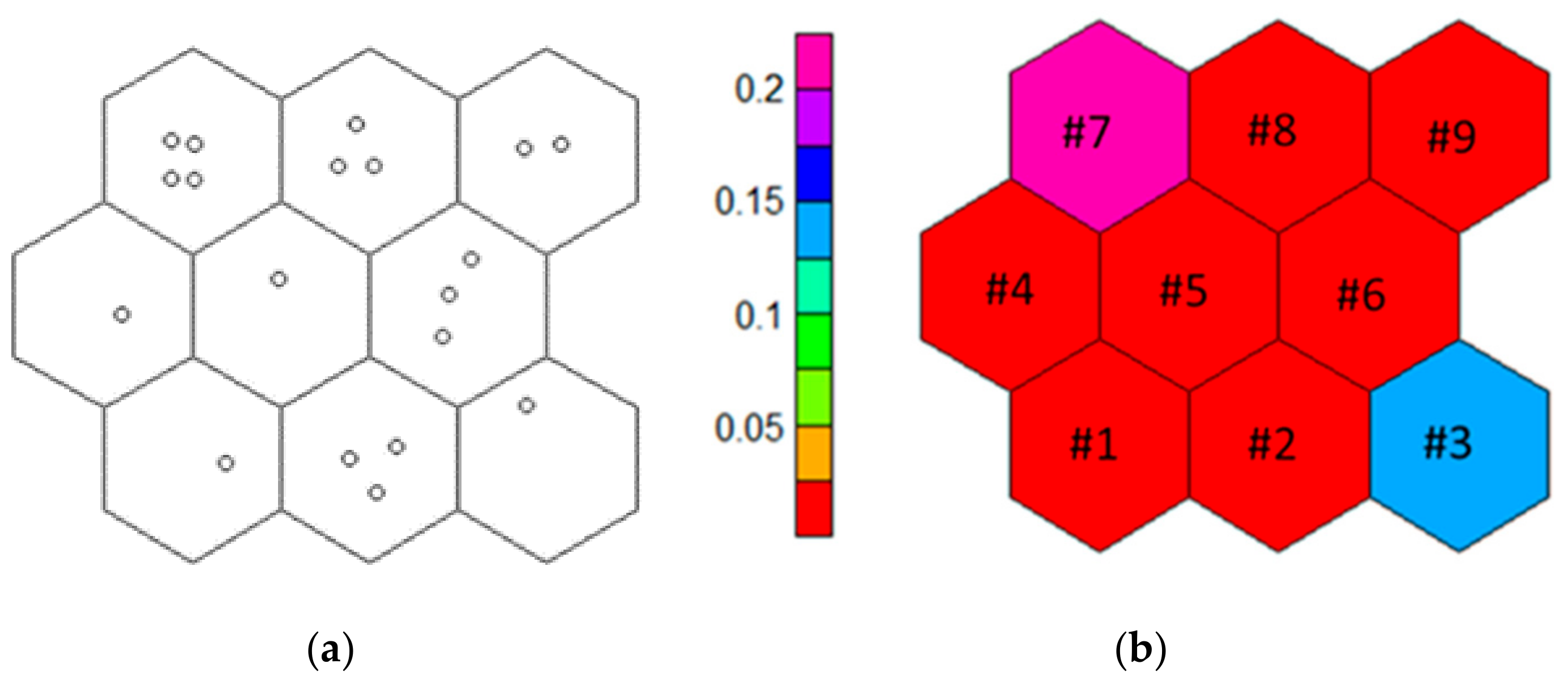
With the aim of creating more accurate up-to-date customer-specific water consumption curves, refined measurement data were used from 21 households in Milford, Ohio, USA. In this context, the SOMs algorithm was applied as the main clustering algorithm and in combination with KM and HAC, optimal clustering was achieved. Specifically, for SOMs clustering, an initial mapping plot was produced, as shown in
Figure 5a, which includes a number of observations (households) in each node. The observations are spatially distributed and their distance from the node codebook vector—the vector formed with values from the features extracted by the dataset for each node—signifies its relevance. We see that there are no empty nodes, which indicates that the map structure is appropriate for the data. The mapping quality is assessed by the quality plot in
Figure 5b which shows the mean distance of objects mapped in a node to the codebook vector of that node; thus, values close to 0 indicate good quality of the SOM. Even for the two nodes shown in blue and magenta colors, the mapping quality is still good (0.2 or less), even though not ideal.
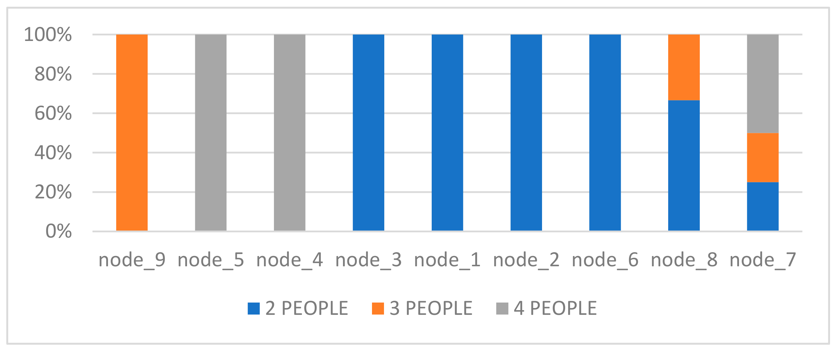
In order to link clustering household characteristics in the dataset and assess clustering accuracy, we test whether the number of people per household varies across SOM nodes. In
Figure 6, we show the variation of number of people per SOM node and we see that indeed it varies across nodes. We also see that clustering could be improved, by combining various nodes in a single cluster, which is already an indication that the KM and HAC algorithms can be used to further cluster data to produce fewer and better clusters.
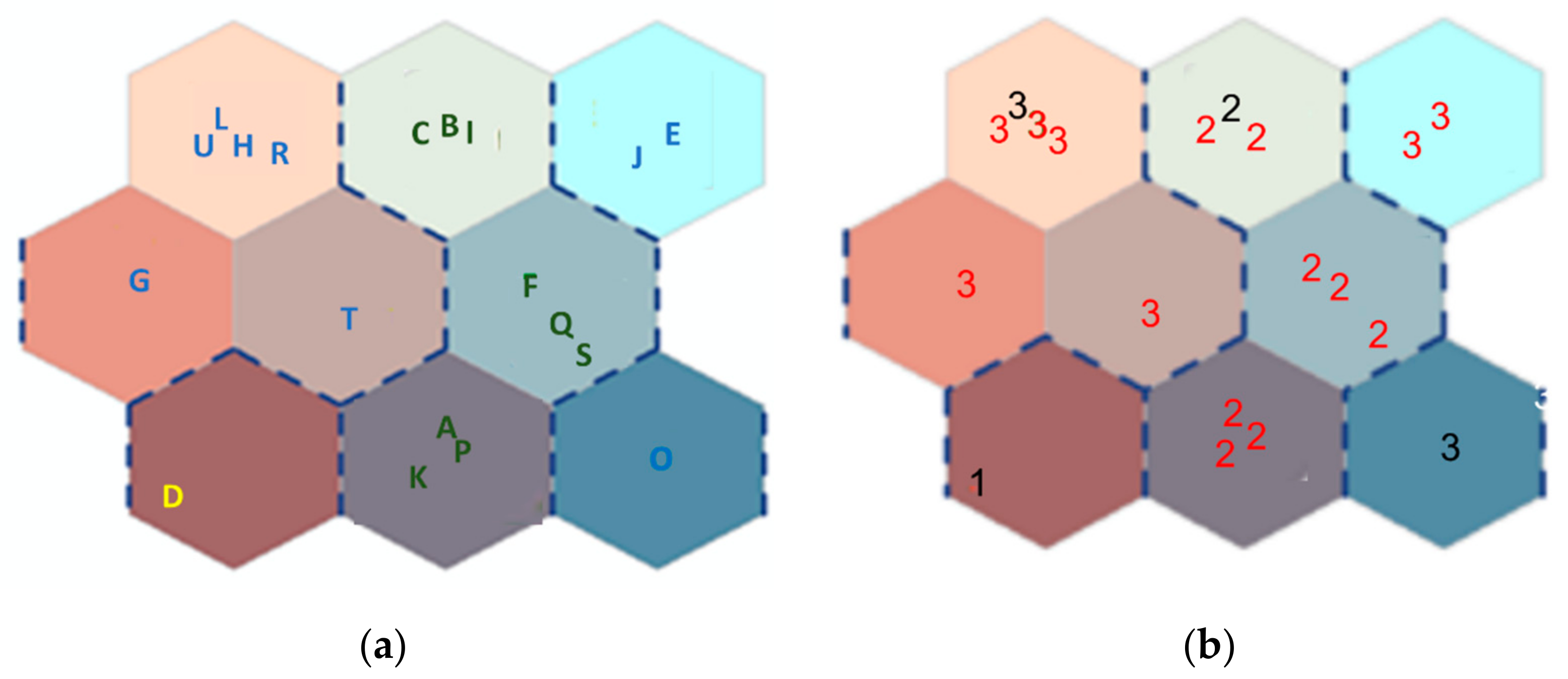
To assess the clustering accuracy of the combined algorithms (SOM-KM, SOM-HAC), we provided the number of people per household and checked how this number corresponds with clustering results. Nineteen households were grouped in 3 clusters—different for each combined algorithm. The accuracy results are 73% and 79% for SOM-KM and SOM-HAC respectively, indicating the SOM-HAC as a slightly better and the preferred clustering solution; calculation of the clustering accuracy is explained below. This does not mean that we reject the SOM-KM clustering technique; we simply choose to present one of the two, in the interest of saving space, namely the SOM-HAC technique. The outcome of the SOM-HAC clustering is presented in
Figure 7a, in which dashed lines group SOM nodes together in larger clusters. This clustering results in the grouping of the codebook vectors or SOM nodes, as shown in the dendrogram in
Figure 4. Cluster 1 contains a single node (#1 per
Figure 5b) and a single household (D)—marked in yellow font. Cluster 2 contains 3 SOM nodes (#2, #6, and #8 per
Figure 5b) and 9 households—marked in green font. Finally, cluster 3 groups 5 nodes (#3, #4, #5, #7, and #9 per
Figure 5b) and 9 households—marked in blue font. This information is also summarized in
Table 3. In
Figure 7b, the algorithm maps the households again, but each entry is represented by its cluster number: therefore, in node #6 for example, instead of showing households F, Q and S (as is done in
Figure 7a), we show the cluster number that these houses belong to. In other words, we show a series of 2s, since all these households belong to cluster #2. All entries in black font signify the households that should not be classified in that cluster, while red entries are the households that are correctly placed in the specific cluster. Clustering accuracy is the fraction of matches (reds) in each cluster for the combined algorithms. Cluster 2 contains mostly 2 residents per household, while cluster 3 contains mostly 3- or 4-people households. When a household with 3 or 4 people is classified in cluster 2, then it is marked black by the algorithm; the same is true for 2-people households classified in cluster 3. So, household L is classified in Cluster 3, even though it should be classified in Cluster 2 (2 residents in household L, as shown in
Table 2); thus, the number 3 that corresponds to household L is shown in black in node #7. Cluster 1 contains only 1 household (D), even after employing the HAC algorithm that improves clustering; since clustering analysis has no meaning for a cluster with a single entry, we decide to not consider this cluster further, dropping household D from further analysis, as an outlier.
4. Discussion
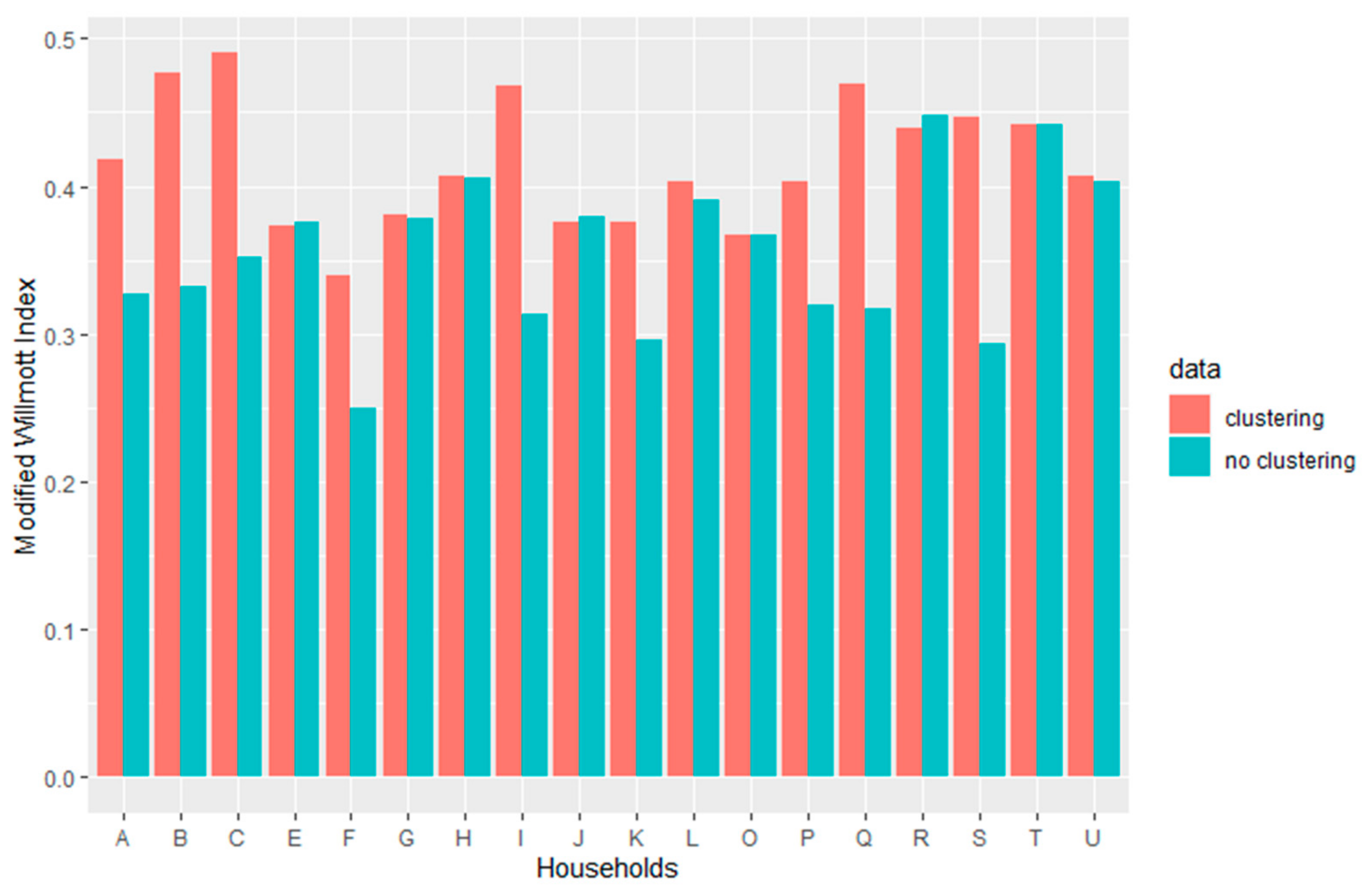
The
WImod is used to assess improvement in estimated customer water consumption achieved through clustering. For each of the 18 households, two
WImod values are obtained: one that examines how the actual water consumption time series matches the cluster-estimated curve and one for the no-cluster-estimated curves. The former curve is calculated by including only households in the cluster, while the latter includes all households (no clustering). In
Figure 8, we see a plot of
WImod for the two cases and we can see that there is an improvement with clustering, which is significant for some households, proving that clustering can lead in obtaining estimated customer water consumption curves that are a closer match to the observed consumptions. Improvement is not observed across the board for all households and this is something that is expected, due to the very limited number of households and the limited duration of the data set (less than a year). The fact that a significant improvement is observed for some households is important and indicates that the methodology presented in this article is promising.
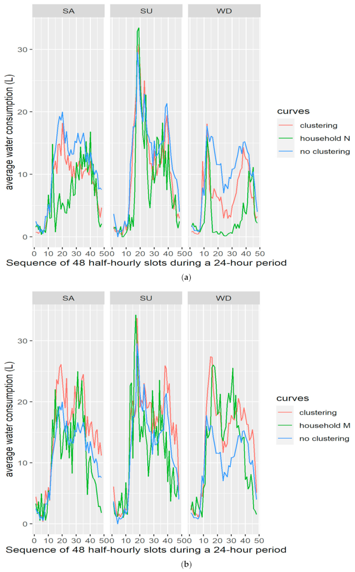
This analysis would be valid for the water utility on existing customers that are grouped based on their historical consumption data. But what about new customers that come without historical time series? In this case, the utility would classify new customers based on the number of people in the household. We do this for the two households that were set aside for validation, namely households M and N. Since household M has 2 people and N has 3, the former would be classified in cluster 2 and the latter in cluster 3. When we perform the same analysis with the curves, we see that household N has an improvement of almost 40% in the
WImod and household M has about 4% improvement in the same index. In
Figure 9a,b, we see how the curves of households M and N are comparatively closer to the curves of clusters 2 and 3, respectively, than the curve obtained for all households, thus validating the clustering methodology. Observing the plots in
Figure 9a,b, one can see that better agreement is obtained on weekday data than on Saturdays or Sundays; this might be a result of more structured activities during weekdays, compared to weekends, when behavior is more stochastic and not characterized by a “typical” schedule that is expected to be followed during work- and schooldays for families. In addition, there are more weekdays than weekends in the dataset, so more data leads to better fitting.
5. Conclusions
Urban water consumption is one of the main concerns of city managers nowadays. Consumer awareness of household water consumption defines consumption behavior and may promote water conservation activities. In this article, we present a novel methodology suitable for handling large datasets of household water consumption. This analysis aims to divide customers into user groups (clusters) based on the similarities of their water use behavior; this way, advanced data-based methods may be employed for creating personalized information about consumer water use.
The presented methodology resulted in better estimates of customer water use when clustering was employed, compared to the predictions when clustering was not employed. This powerful information can provide a lot of insight to water companies, as it allows them to have knowledge of water demand in a detailed spatio-temporal granulation, thus promoting good planning and efficient operation. Water companies have better knowledge on what to expect from new customers, by classifying them in pre-existing clusters; they can obtain information on pumping energy needed and they have rich datasets that could be used for modeling the water distribution network, for reducing leakage, for optimizing treatment and pumping, for accurate billing, and for prioritizing investments.


