
COVID-19 Pandemic Turns Life-Science Students into “Citizen Scientists”: Data Indicate Multiple Negative Effects of Urbanization on Biota


iES Landau, Institute for Environmental Sciences, University of Koblenz-Landau, 76829 Landau, Germany
Sustainability 2021, 13(5), 2992; https://0-doi-org.brum.beds.ac.uk/10.3390/su13052992
Submission received: 25 January 2021
/
Revised: 4 March 2021
/
Accepted: 5 March 2021
/
Published: 9 March 2021
Abstract
:The COVID-19 pandemic and its restrictions strongly affect the higher education community and require diverse teaching strategies. We designed a course where we combined online teaching with independently conducted ecological data collections by students using a “citizen science” approach. The aim was to analyze the impact of urbanization on biota by comparing urban and rural grasslands. Seventy-five students successfully conducted the data collections and the results provide evidence for prevailing negative effects of urbanization. Individual numbers of ground-dwelling invertebrates (−25%) and pollinating insects (−33%) were generally lower in urban sites. Moreover, animal and seed predation were reduced in urban grasslands, indicating the potential of urbanization to alter ecosystem functions. Despite the general limitations of online teaching and citizen science approaches, outcomes of this course showed this combination can be a useful teaching strategy, which is why this approach could be used to more actively involve students in scientific research.
1. Introduction
The COVID-19 pandemic affects all aspects of our life and has detrimental impacts on human health and the global healthcare system. Moreover, the restrictions in order to slow the spread of the pandemic—lockdown, social distancing, travel restrictions, self-quarantine, and many more—have tremendous socio-economic consequences [1]. These include all levels of education and create significant challenges for the higher education community [1,2]. As one consequence, universities worldwide have closed (or postponed) campus events and moved to online teaching [2,3].
Online teaching offers great opportunities and has multiple advantages for both lecturers and students. It may reduce costs, allow lecturers to teach from various locations, enables students to flexibly access the material at any time and location, and reduce stress by offering self-pacing opportunities for the learners [4,5]. On the other hand, online teaching often requires more efforts by the teachers and learners, is impersonal by lacking physical interactions between teachers and students and among students, requires a high level of self-discipline, and depends on the IT equipment and resources of both the universities and the students [3,4,5]. Furthermore, online teaching is complicated especially for practical courses, where specific equipment and materials are required (e.g., microscopes or measuring devices in the laboratory). Facing these challenges, our motivation was to develop a teaching strategy for a practical seminar for life-science students (University of Koblenz-Landau, Germany) and to offer the course during the COVID-19 pandemic in the summer semester of 2020. The basic aim of the course “Organisms and their environment” is that students learn practical fieldwork related to current ecological questions. Thus, we combined the online provision of theoretical input by the teachers (lectures, videos, sampling protocols, etc.) with inquiry-based learning by the students (independently conducted practical fieldwork). Most of the students were in the early semesters of their bachelor´s program and had virtually no experience in ecological fieldwork. Moreover, many of them were working from their home residences because of the lockdown of the campus and travel restrictions and, thus, had no access to the university’s scientific measuring equipment. We, therefore, conceived the fieldwork part of the course using a “citizen science” approach (see Section 2.1, Figure 1).
Citizen science is well suited to connect authentic scientific research with science education [6,7]. In particular, the active engagement of students within citizen science projects can stimulate their awareness of environmental and ecological issues [6,7]. Students collecting data as a part of a course are being compensated in the form of their grades and therefore are not simply volunteering. Whether students can be considered as citizen scientists might be questionable and depend on the underlying definition of citizen science. However, there is no single definition of citizen science but rather a series of definitions and it can be interpreted in many different ways [8,9]. In this paper, I interpret citizen science as the involvement of non-professionals in scientific research, which implies also university students participating as part of their coursework [6]. Citizen science has been shown to provide very useful data in ecological science [10,11,12,13]. Ecological citizen science projects range from the global scale (such as bird monitoring programs) to local scales with investigations of various organism groups [10,13,14]. Citizen science provides valuable information in biodiversity research [13] and seems to be especially useful for urban ecological questions [6,10,15,16,17].
In view of the increasing global trend of urbanization, urban ecology and biodiversity research are of great interest and some of the most important fields in environmental research [18,19,20]. Urbanization strongly influences environmental conditions and cities are characterized by higher temperatures (“urban heat island effect”), increased surface run-off of rainwater, increased soil pH, and enhanced air, light, and noise pollution—to mention just a few prominent examples [21,22]. Urbanization with its associated environmental alterations is thus regarded to be a major threat to biodiversity [23,24,25,26]. On the other hand, cities can provide habitats for a great number of species [27,28,29] and may remarkably contribute to biodiversity conservation [19,30,31]. Understanding urban biodiversity dynamics is thus paramount to assess the role of cities in biodiversity conservation [19,32]. Moreover, urbanization not only affects biodiversity but may strongly alter ecosystem functions [33]. For example, Knop et al. [34] showed that increased light pollution—as a consequence of urbanization—can reduce the pollination service by moths and Fischer et al. [35] demonstrated that predation by vertebrates is reduced in urban environments.
With this paper, I want to show that the students acted as engaged citizen scientists and provided a robust dataset. Using this dataset, I will provide evidence that urbanization has multiple negative effects on biota. Moreover, the results confirm the expectation of strongly altered environmental conditions in urban habitats compared to rural counterparts.
2. Material and Methods
2.1. Teaching Strategy and Workflow of the “Citizen Science” Approach
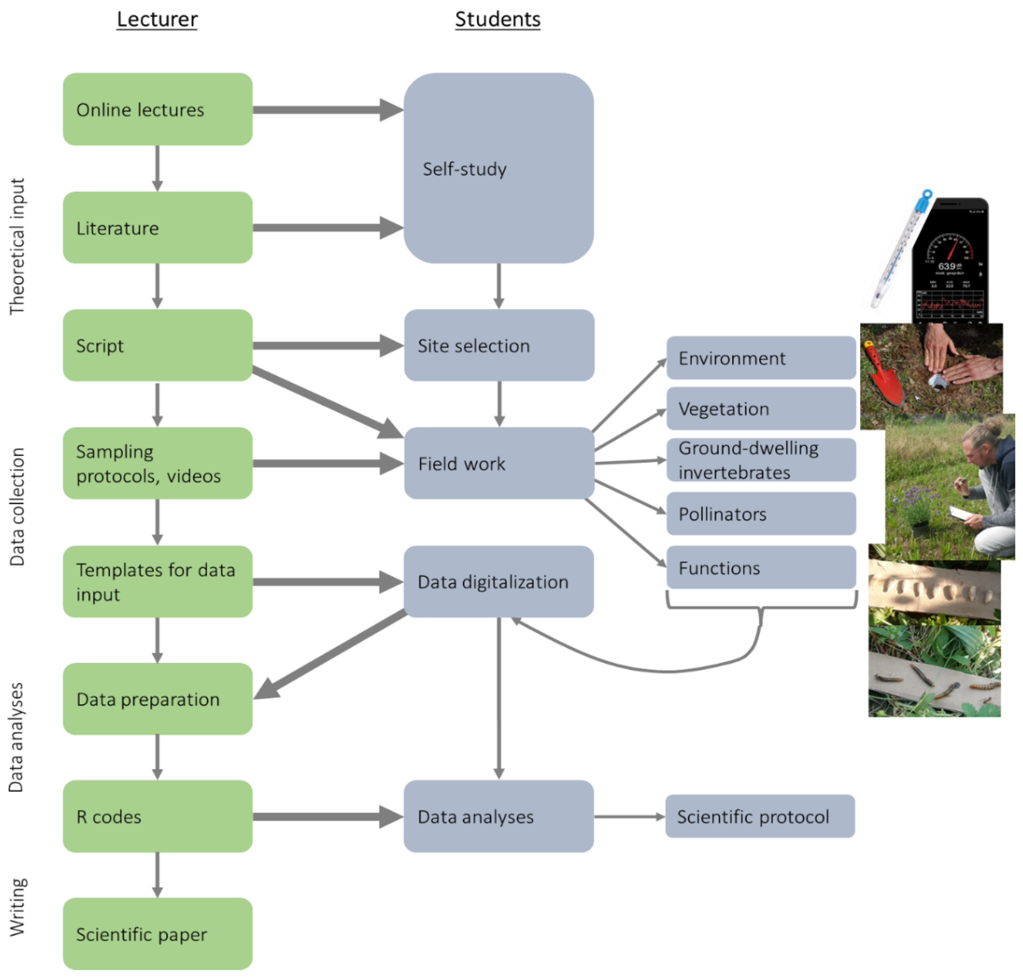
The project was done in the summer semester of 2020 within the universal course “Organisms and their environment” of the iES Landau, Institute for Environmental Sciences, University of Koblenz-Landau (Germany). In total, 93 life-science students of the study programs “Environmental Sciences” (Bachelor of Science, N = 59 students), “Biological Conservation” (Bachelor of Science, N = 17), and “Biology” (Master of Education, N = 17) participated in the course. Due to the COVID-19 restrictions, face-to-face teaching, personal meetings (even in smaller groups), and the provision of material or scientific devices to the students were not possible. Thus, we decided to conduct the course in a way, where the lecturers provided theoretical input and instructions via online teaching and the students conducted independent data collections as a form of “citizen science” (Figure 1). Importantly, the students should be able to collect data and take measurements with simple, freely available, and affordable materials and methods (free apps for smartphones, household devices, free software, etc.). The descriptions regarding the study design and data collection given in this paper (Section 2.2 and Section 2.3) were provided online to the students in form of a script, videos, and precise sampling protocols (Figure 1). Therefore, and for all further communications like a chat for contacting all course members or a contact form to communicate with the teacher, the open learning management system “OpenOlat” was used (frentix GmbH, Zürich, Switzerland).
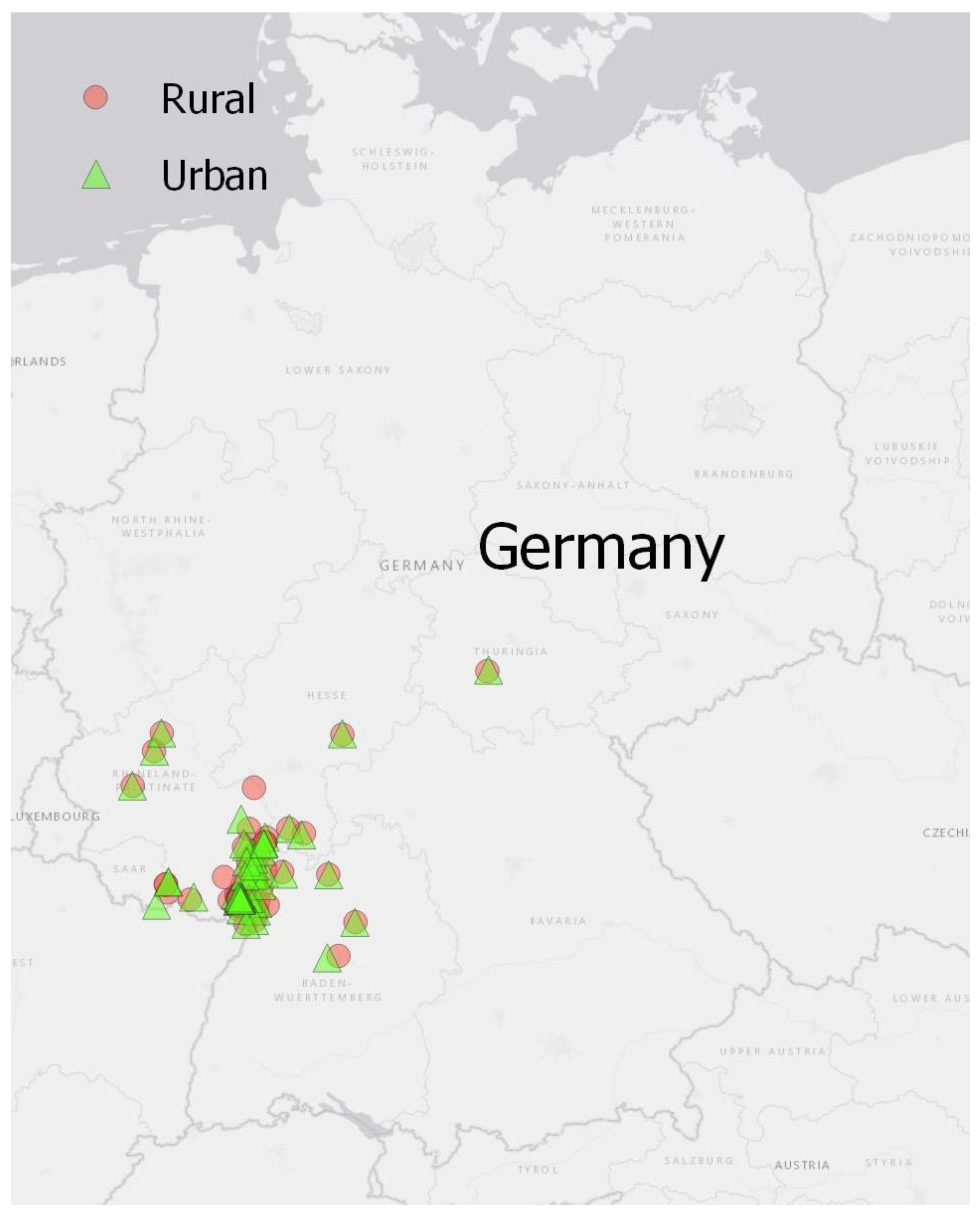
We focused on the topic “urbanization effects on biodiversity” mainly for two reasons. First, the contemporary decline of biodiversity is one of the most salient fields of current ecological research [36,37,38,39,40]. By focusing on urban ecology, a subject of immediate relevance to the experiences of our students, we hoped to motivate them, since “helping the environment” turned out to be one of the major motivations to support citizen science projects [41]. Second, due to the COVID-19 restrictions, we assumed that many students would not be living close to the university campus (Landau) but in their hometowns distributed all over Germany. However, all students should be able to conduct the course, irrespective of their current residence. We believed that collecting data in urban and rural grassland site pairs would be possible for all students. Indeed, it turned out that students conducted the data collections in 26 districts across 5 German federal states (Figure 2).
2.2. Site Selection
Urban and rural sites were selected by the students according to the following criteria: (i) only open grassland sites were allowed. Grassland usually covers large areas in urban environments, often harbors species- and individual-rich biotic communities and has therefore potential for urban biodiversity conservation. (ii) Urban and rural grasslands should be of a similar and comparable vegetation type (e.g., road verge, meadow, fallow). (iii) Urban sites should be located between the city center and the city edge. The cover of impervious surfaces (buildings, streets, etc.) in the surrounding (buffer with 200 m radius) should be at least 30%. It turned out, that the selected urban sites had an impervious surface cover of 61.7 ± 1.9 (minimum: 30%, maximum: 90%). (iv) Rural sites should be located in the cities’ adjacent rural landscapes or at the city edge. They should have an estimated impervious surface cover in the surrounding area of a maximum of 30%. In the end, the selected rural sites by the students had on average a cover of 9.5 ± 0.8 impervious surfaces in 200 m surrounding (minimum: 0%, maximum: 30%). Estimations of the % impervious surface in the 200 m buffer around urban and rural sites should be done using free satellite images (e.g., Google Earth, Google LLC, Mountain View, CA, USA; Zoom Earth, Neave Interactive Ltd., Brighton, UK). (v) Site pairs should have a comparable size and be at least 100 m² in size.
2.3. Data Collection
Data collections were done on three consecutive calendar weeks (24–26) in June 2020. Each student had to visit each site on one day in calendar week 24 and 26, respectively, and on two consecutive days in calendar week 25. Thereby, the sites were visited in an alternate order to minimize systematic biases of daytime. Data collections were done in the center of each site.
2.3.1. Environmental Parameters
The noise level was recorded using a free software for smartphones (e.g., Sound Meter App, Abc Apps, Wilhelmshaven, Germany). Measurements were done on each site visit. Per visit, the noise level was measured three times every 30 min for 60 s. Afterwards, the average noise level in dB was calculated to obtain one value per site.
The temperature was measured using simple thermometers for household uses (e.g., compost, soil, or meat thermometers). The temperature was measured (a) on the soil surface and (b) at 5 cm soil depth. The measurements were done three times on each visit following the measurements for the noise level. Afterwards, the average temperature on the soil surface and at 5 cm depth were calculated.
As an indirect measure of light pollution, the distance from the center of the sites to the nearest artificial light source (street lamps, illuminated shop windows, etc.) was calculated (m) at the first visit of the sites. This could be either done by measuring the distance in the field by using steps (one big step ~1 m) or by measuring the distance using free software with satellite images or maps (e.g., Google Earth; OpenStreetMap, OpenStreetMap Foundation, Cambridge, UK).
2.3.2. Ellenberg’s Indicator Values
Ellenberg’s indicator values [42] were used to further characterize the abiotic site conditions. Ellenberg’s indicator values are frequently used in Central European ecological studies for the assessment of environmental conditions without direct measurements. In this system, the ecological optima of plant species are expressed as ordinal numbers. Average values of Ellenberg’s indicator values calculated for a vegetation sample can therefore reflect environmental conditions at a site [43]. In calendar week 24, per site 10 randomly chosen plants were determined up to species level and their Ellenberg indicator values were assessed online (http://statedv.boku.ac.at/zeigerwerte/). Afterwards, the mean site indicator values were calculated for light, temperature, humidity, nitrogen, and reaction. For plant determination, standard identification keys were used in combination with free apps for smartphones (e.g., Pl@ntNET, plantnet-project, France; Flora Incognita, Technische Universität Ilmenau, Ilmenau, Germany).
2.3.3. Vegetation Structure
To characterize the vegetation structure the cover of the field layer, cryptogams, and litter was estimated (%) in a 2 × 2 m plot in the center of each site (calendar week 24). To support the students with the visual inspection, an auxiliary table was provided [44]. In addition, the height of the field layer was measured at five randomly chosen points per plot with the drop disc method, a very objective and simple method for measuring the vegetation height [45]. Specifications for the use of the drop disc were: prepared from cardboard, diameter of 17.5 cm, and a ~2 cm hole in the center. The disc was always dropped from 1 m height along a stick (e.g., folding rule) and for further analyses, the average height of the five measurements per site was used.
2.3.4. Ground-Dwelling Invertebrates
Ground-dwelling arthropods were captured with pitfall traps. The traps were installed during one day in calendar week 25 and left open until the morning of the next day (~15 h exposition time). In the center of each site three traps were placed in form of a triangle with a 2 m distance. No trapping liquid was used because we did not want to kill organisms, which were not further used for identification. Instead, students sorted the trapped organisms directly in the field into five easily recognizable and abundant ground-dwelling invertebrate groups and counted their individual numbers: spiders (including harvestmen), beetles, ants, millipedes, and woodlice. Afterwards, all trapped individuals were released. We provided pictures and short fact sheets with the most important identification characteristics of the groups as a field guide to the students.
Snails and woodlice were detected by placing one wooden board (size: ~0.25 m2) per site as a shelter trap. The wooden boards were placed in calendar week 25 and burdened with a stone. After one week, the bottom side of the boards were checked for snails and woodlice and all individuals were counted. For statistical analyses, the individual numbers of captured woodlice from the pitfall traps and the wooden boards were summed.
2.3.5. Pollinators
Pollinating insects were observed on one day in calendar week 26 using sentinel plants. The observations were allowed to be conducted only under suitable weather conditions (dry, warm, calm). For the observations, a potted and flowering lavender plant was placed in the center of each site. If the students were not able to buy a flowering lavender plant in a market garden, supermarket, etc., they were allowed to use any other potted flowering labiate plant species (e.g., sage, thyme). After a waiting time of approximately 15 min, all flower-visiting and potential pollinating insects were counted for 30 min. When an individual only inspected a flower from a distance and obviously did not interact with the flower, this was not counted as a flower visit. When one individual successively visited several flowers, this was counted as one visit. Pollinators were classified into bees (including honey bees), bumblebees, wasps, butterflies, hoverflies, other flies, and beetles. For help with the identification, the students could use common field guides and/or free identification apps such as the German “NABU-Insektenwelt” (Mullen & Pohland GbR, Wülfrath, Germany), which also allows offline identification.
2.3.6. Animal and Seed Predation
Predation and seed predation were assessed as two important ecosystem functions. Therefore, sentinel preys were used with mealworm beetle larvae (animal predation) and sunflower seeds (seed predation). Sentinel systems are frequently used in ecological studies to assess predation rates [46,47]. Bait sticks were prepared from cardboard with a size of 15 × 3 cm. On the bait sticks used for measuring animal predation, seven larvae of the mealworm beetle (Tenebrio molitor) were stuck, evenly distributed with a little superglue. Mealworm larvae were used because of their good availability in online pet shops etc. For seed predation, 10 sunflower seeds were stuck on the cardboard sticks. Per site three bait sticks for animal and seed predation, respectively, were placed on the ground and fixed with wooden skewers or toothpicks. The bait sticks were exposed during one day in calendar week 25 (same date as for the pitfall traps) and checked in the morning of the next day (15 h exposition time). The number of eaten mealworm larvae and sunflower seeds were counted and the % predation per site calculated.
2.4. Data Validation and Analysis
Of 93 registered students, 79 students uploaded the data. Data was uploaded on the learning platform “OpenOlat” by the students using provided templates. All data was validated by the teacher and typos (e.g., false decimal separator) and obvious errors (e.g., “cm” instead of “m”) were corrected. Missing values (e.g., not all students were able to measure temperatures, lost wooden board) were indicated with NA´s (not available). Thereby, NA´s were inserted always for both sites (also when measurements were not available only for one site) to account for the paired study design and analyses (see below). Four datasets were excluded because they contained too many missing or unrealistic values. The total dataset for analyses, therefore, comprised samples from 75 grassland site pairs (Supplementary material Table S1).
All statistical analyses were performed using R version 3.6.1 [48] by the author. A p-value < 0.05 was considered as statistically significant, a p-value < 0.1 as a trend. Means ± one standard error (SE) are given unless differently specified.
Differences in environmental parameters (noise, distance to next artificial light source, the temperature on the soil surface and at 5 cm depth), Ellenberg indicator values of plants (light, temperature, humidity, nitrogen, reaction), vegetation structure (field layer cover, cryptogam cover, litter cover, the height of field layer), and animal and seed predation between urban and rural grassland sites were tested with linear mixed-effects models (command “lmer” in R package lme4, [49]). To test differences in individual numbers of ground-dwelling arthropods and pollinators between urban and rural sites, general linear mixed-effects models with a negative binomial distribution were applied (for count data and detected overdispersion; command “glmer.nb” in R package lme4. Because of the paired study design—each student sampled an urban-rural site pair —a random effect indicating the paired location was included in the models. Using these kinds of mixed-effects models, therefore, accounts for some sampling bias (e.g., differences in estimation rates among students), and has been proven to be very useful in analyzing citizen science data [50]. The p-values are based on subsequent ANOVA (chi-square)-testing (command “Anova” in R package car; [51]).
3. Results
3.1. Environmental Parameters, Ellenberg Indicator Values, and Vegetation Structure
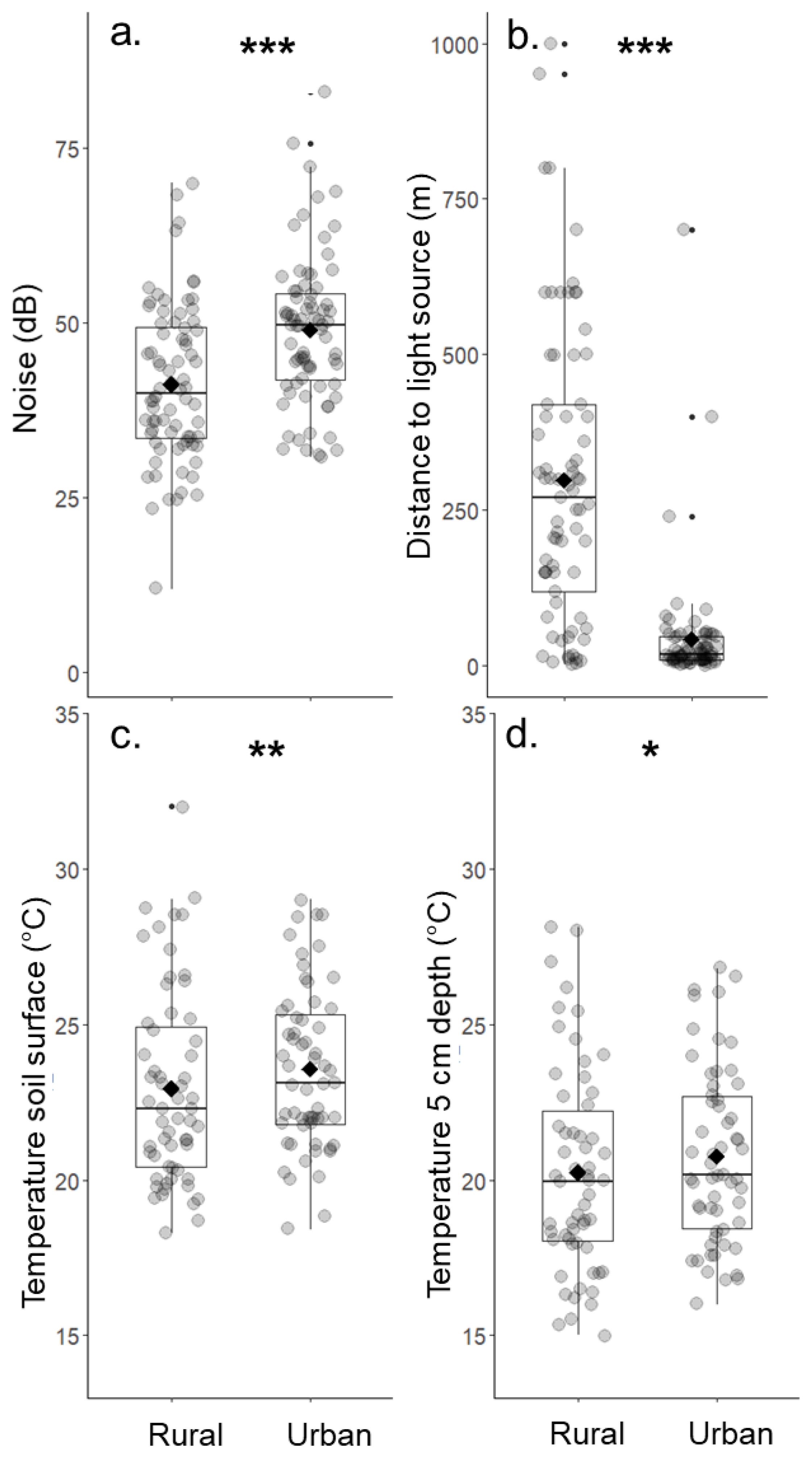
All four environmental parameters significantly differed between urban and rural grassland site pairs (Table 1). On average, the background noise level was almost 8 dB higher in the urban grassland sites compared to rural sites (Figure 3a). The distance of the grassland sites to the next artificial light source at night also differed significantly between urban and rural site pairs. Urban grassland sites had a mean distance of 43 m while rural sites were on average 321 m away from a light source (Figure 3b). As expected, the temperature was significantly higher in urban sites compared to the rural ones. The temperature on the soil surface was 0.6 °C and the temperature at 5 cm soil depth 0.5 °C higher in the urban grasslands (Figure 3c,d).
The comparison of the Ellenberg indicator values between urban and rural grassland sites revealed no significant differences (Table 1). However, we found trends for lower mean values for humidity and reaction in urban compared to rural grassland sites.
3.2. Individual Numbers of Ground-Dwelling Invertebrates and Pollinators
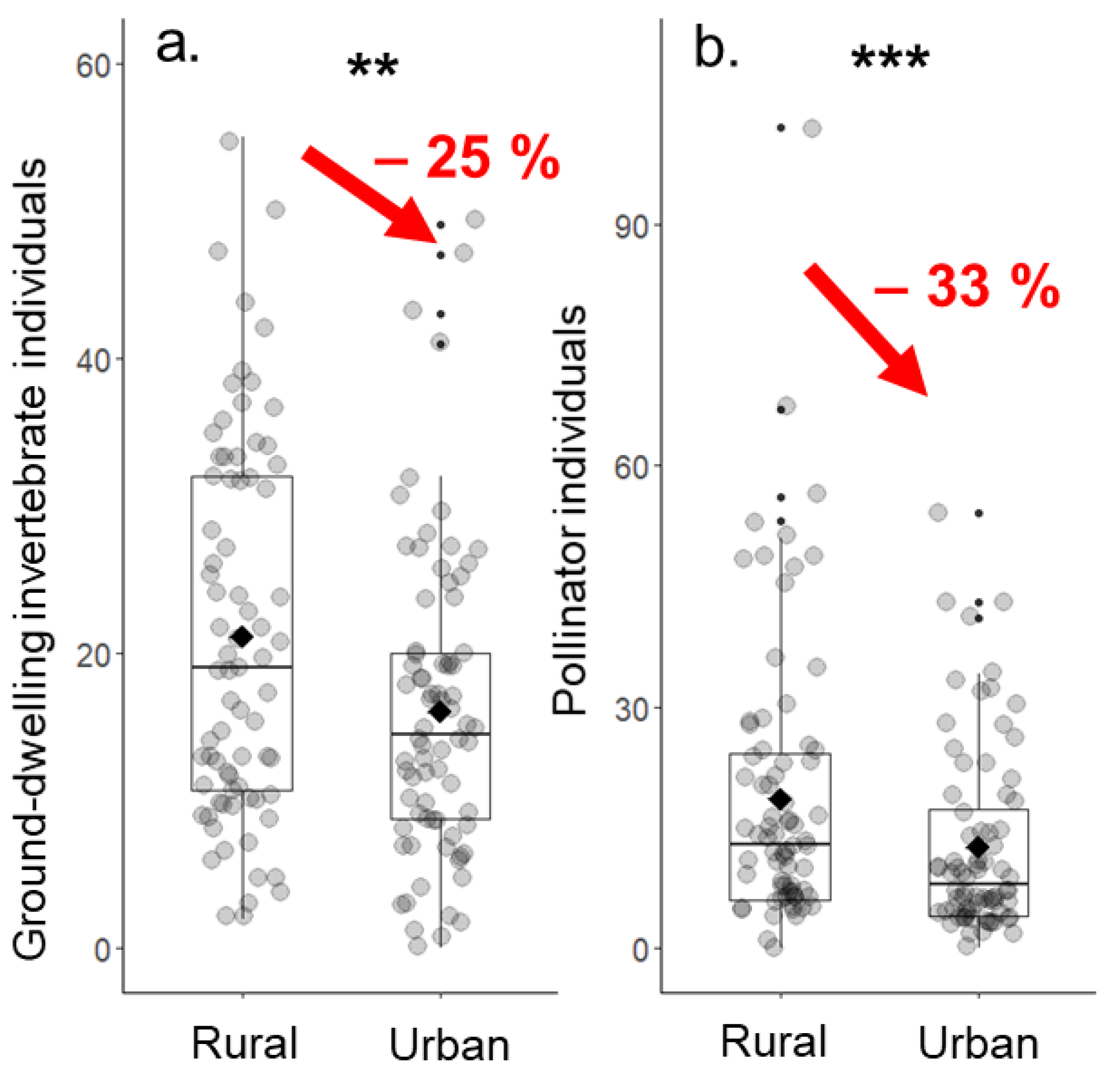
Individual numbers of ground-dwelling invertebrates were lower in urban grassland sites compared to rural ones. This effect was significant for total individual numbers (−25.4%, Figure 4a), beetles (−42.7%), millipedes (−63.6%), and woodlice (−34.2%), but not for spiders (−15.2%), ants (−6.1%), and snails (−5.0%).
Similarly, the individual numbers of pollinating insects strongly differed between urban and rural grasslands. The number of total pollinators was significantly reduced in urban grassland sites and on average 32.6% lower (Table 2, Figure 4b). Similar significant patterns were found for all analyzed pollinator groups except for other flies (Table 2). The significant reductions in individual numbers from rural to urban sites ranged from −57.6% for butterflies to −23.3% for hoverflies. Significant values (p ≤ 0.05) are shown in bold.
3.3. Animal and Seed Predation
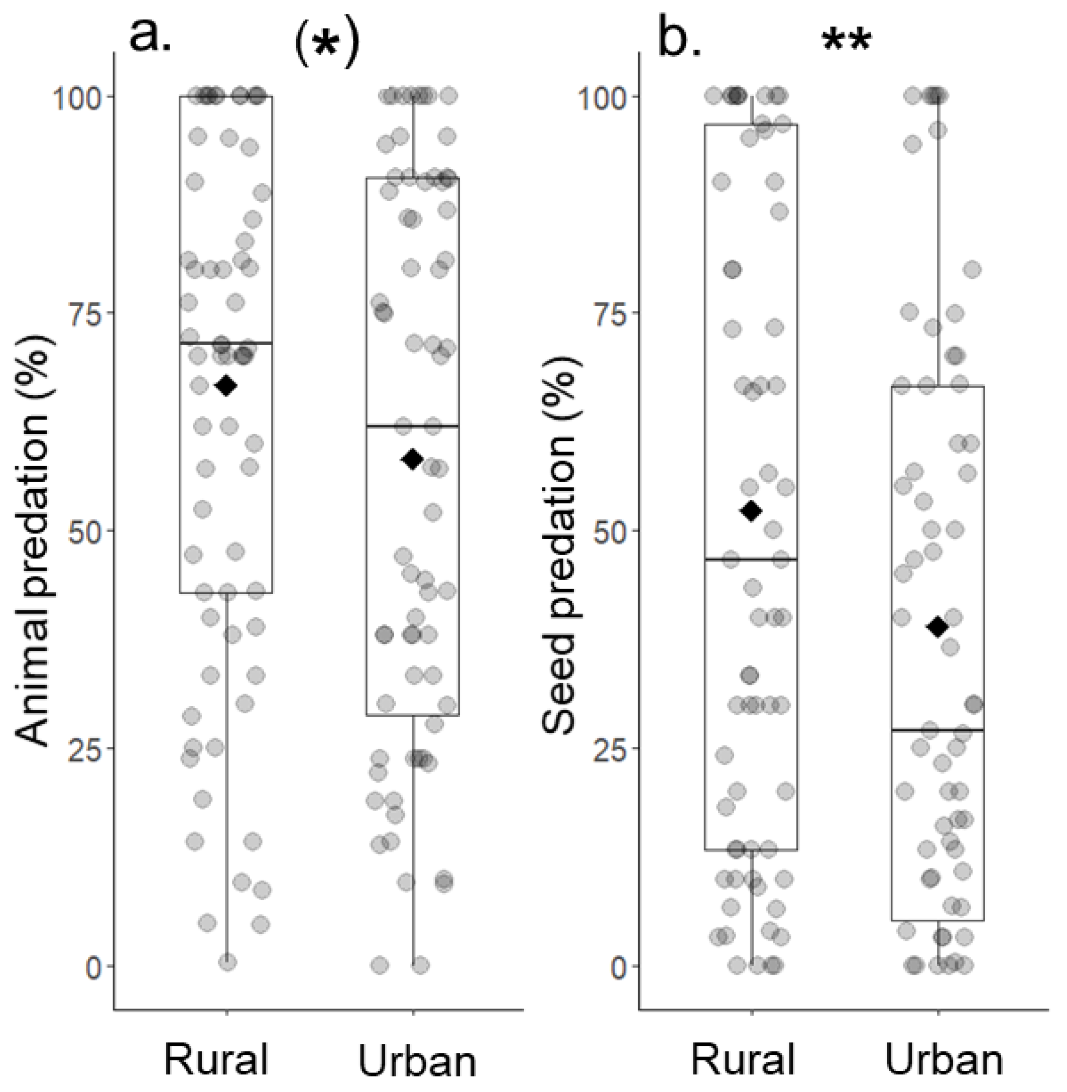
Animal predation tended to be lower in urban (57.8 ± 3.9) compared to rural (67.1 ± 3.6) grassland sites (N = 74, Chi² = 3.74, p = 0.053, Figure 5a). Seed predation was significantly reduced in urban (38.8 ± 4.2) grasslands and about 25% lower than in rural sites (52.6 ± 4.5) (N = 74, Chi² = 7.22, p = 0.007, Figure 5b).
4. Discussion
4.1. Multiple Negative Effects of Urbanization on Biota
Cities can provide habitats for a great number of species [27,28,31] and support individual-rich communities [21,32,52]. Thereby, especially urban grasslands might play an important role in conserving urban biodiversity [53], since they often cover large areas in cities, and management measures targeted for conservation can be applied and adapted quickly and easily [54].
However, the results of this study—based on ‘citizen science’ data from life-science students—provide evidence for prevailing negative effects of urbanization on biota. Overall individual numbers of ground-dwelling invertebrates (−25%) and pollinating insects (−33%), as well as predation rates, were generally lower in urban grassland sites compared to corresponding rural sites. Thus, the present study supports the findings of recent meta-analysis and large-scale studies, which also revealed predominantly negative effects of urbanization on animal diversity and abundances [26,55,56]. Saari et al. [55] showed that the overall abundance of terrestrial animals is generally lower in urban sites compared to rural ones. Similarly, Fenoglio et al. [26] found reduced abundances in urban habitats when focusing on terrestrial arthropods. Additionally, this meta-analysis demonstrated the negative effects of urbanization on overall arthropod diversity. The main factors explaining reduced animal abundances in urban environments are habitat loss (e.g., construction of impervious surfaces), increased habitat fragmentation and isolation (e.g., remaining suitable habitats as small and isolated remnants with the urban matrix), and habitat degradation (e.g., pollution with contaminants, light pollution, noise pollution) [26,55]. Reduced abundances for herbivorous and pollinating insects might further be explained by the high abundance of non-native plant species in urban habitats [18,57]. Non-native plants often support fewer herbivore (insect) species and abundances than native plants [58,59,60].
The influence of urbanization on diversity and individual numbers has been shown to be taxa-dependent [26,61,62]. One aim of this study was therefore to use a multi-taxonomic approach with simultaneous investigations of a broad range of invertebrate organism groups. Regarding ground-dwelling invertebrates, significant and substantial reductions in individual numbers were found for three out of six investigated ground-dwelling arthropod groups, namely beetles (−43%), millipedes (−64%), and woodlice (−34%). Regarding beetles, this confirms findings of Fenoglio et al. [26], where beetles also belonged to the most affected groups. In addition to the factors mentioned above (especially soil pollution), elevated temperatures and lower humidity in cities can explain the negative (interactive) effects on these groups, since the majority of millipede and woodlice species, and also several (ground) beetles, are moisture-dependent [63,64]. Moreover, plant quality and quantity are important drivers for millipedes and woodlice [63], which might be reduced in the studied urban grasslands as indicated by the lower field layer height (Tab. 1). Low and statistically non-significant reductions were observed for spiders, ants, and snails. Spider abundances seem to be generally less impacted by urbanization [26], possibly, because some generalist (wolf) spiders can exploit urban habitats contributing to individual-rich communities [65]. Regarding pollinator abundances, this study revealed very consistent negative effects of urbanization. Except for flies (other than hoverflies), individual numbers of all investigated groups were significantly lower in urban sites compared to rural ones. The most severe reduction was observed for butterflies (−58%). This is in line with the results of Fenoglio et al. [26], where Lepidoptera were also highly affected by urbanization. This was explained mainly by their close relationships to host plants (especially during the larval stages), and sensitivity to microclimatic conditions. Surprisingly, strong reductions in abundances were observed for bumblebees (−48%), wasps (−38%), and beetles (−29%), since recent studies emphasize the value of cities for pollinators [28,52,66].
The observed reductions in invertebrate abundance and diversity in cities (this study, [26,55]) might influence ecosystem functioning, trophic interactions, and the provision of regulating services, such as pollination and biological pest control [33,34,35,67]. Here, animal and seed predation were lower in urban grasslands than in rural sites. This might be linked to the observed reduced individual numbers of invertebrates [68], but could have course also be related to the foraging activity of other predators such as mammals or birds. Nevertheless, this finding adds important information on how ecosystem functions can be affected by urbanization, a topic generally understudied in urban environments [69,70].
4.2. Students as “Citizen Scientists”—Strengths and Advantages
Citizen science is useful to combine scientific research with life-science education [7,11]. Based on my experience with this course I agree with this for the following reasons. The students became aware of the current important ecological topics “urbanization effects” and “biodiversity crisis” not only via online theoretical input but also during their practical fieldwork as citizen scientists. Thereby they gained skills and information about practical sampling, observation, identification, and measurements. Moreover, they learned tools to analyze their “own” data and to understand organism-environment relationships and they trained their scientific writing skills (Figure 1). Besides the detected predominant negative impacts of urbanization on ground-dwelling invertebrates, pollinators, and predation (see Section 4.1), the students confirmed basic knowledge of how urbanization affects the environment (Table 1). Using simple measurements (e.g., smartphone apps or household devices), they were for example able to support the urban heat island effect and higher noise pollution in cities (Table 1, [21]). An online evaluation of the course by the students (N = 41, 29 October 2020) showed that 78% of the students agreed with the statement that the course can reasonably be conducted in a digital format and 80% of the students stated that they would participate again in the course if it would be conducted in the same way. According to Dickinson et al. [11], the success of citizen science projects depends on the comprehensible provision of background information (ideas and theories), research questions, and sampling protocols. Therefore, much effort has been made to provide digital lectures, video tutorials, a script, and sampling protocols (Figure 1), which was highly appreciated by the students. Regarding the question, if the provided materials were helpful, 24 students gave the best grade (1 = best, 5 = worst; mean grade: 1.83) in the online evaluation. The overall grade of the course was 1.88 (1 = best, 5 = worst). In summary, I inferred that most students were satisfied with the teaching strategy, which combined the online provision of theoretical input by the teachers with inquiry-based learning by the students.
4.3. Students as “Citizen Scientists”—Limitations
Nevertheless, the current teaching strategy with its “citizen science” approach has some disadvantages. In general, citizen science data has limitations and data analyses can be challenging [10,50]. Concerns often relate to varying skills of observers (e.g., identifying and counting of individuals) and sampling biases (e.g., effort in space in time) [10,71]. The latter issue is of minor importance in the present study since sampling effort and time were standardized due to the provision of detailed protocols. Possible problems with observer errors were accounted for by using the paired study design and the application of (generalized) linear mixed effect models. The provision of educational material (lectures, protocols, videos, etc.) and the data validation were very time-consuming for the teacher (approximately one-third extra time). In comparison to large-scale citizen science projects with thousands of volunteers, the sample size of this study is of course rather low with observation data of 75 students. It is also clear that the results of this study are based on a snapshot analysis, where field observations were conducted only in June of one season. Finally, identification of organism groups could be done only on course taxonomic levels and no information on species level is available.
5. Conclusions and Outlook
The COVID-19 pandemic has strong effects on the higher education community and requires diverse online teaching strategies. For life-science students, the combination of (a) online teaching (provision of theoretical input and instructions by the lecture) and (b) independently conducted ecological data collections by students in a “citizen science” manner framed in an “urban ecology” context can offer great opportunities. It revealed that students acted as engaged “citizen scientists” and provided a robust dataset showing multiple negative effects of urbanization on biota, which is why this approach could be used to more actively involve students in scientific research.
Due to the current situation of the COVID-19 pandemic, we expect an “online” semester also for summer 2021. Based on the positive experiences, I definitely intend to repeat the course “Organisms and their environment” in a similar manner described in this article. Of course, I will try to improve the course based on the experiences and suggestions of the students. Even after overcoming the COVID-19 pandemic crisis and when classroom teaching is again possible, I will include the “citizen science” approach in this course. As a vision for the future, this approach will evolve to a long-term monitoring project where not only students but also the general public can participate. Students can contribute to citizen science projects not only by collecting data, but also, for example, by helping to improve sampling methods and analyzing and visualization of data. I am convinced that university students can take an important role in future citizen science projects and expect mutual benefits.
Supplementary Materials
The following are available online at https://0-www-mdpi-com.brum.beds.ac.uk/2071-1050/13/5/2992/s1. Table S1 contains the data used in this study.
Funding
This research received no external funding.
Institutional Review Board Statement
Not applicable.
Informed Consent Statement
Not applicable.
Data Availability Statement
The data presented in this study is available in Table S1 in the supplementary material.
Acknowledgments
Many thanks to all participating students for their engagement, criticism, and praise. I thank Verena Rösch for her help in designing the course and her acting talent in the video tutorials for the students. I like to thank Sascha Buchholz for helpful discussions on the sampling protocols and Martin H Entling and Leonhard DuBois for comments on the manuscript.
Conflicts of Interest
The author declare no conflict of interest.
References
- Nicola, M.; Alsafi, Z.; Sohrabi, C.; Kerwan, A.; Al-Jabir, A.; Iosifidis, C.; Agha, M.; Agha, R. The socio-economic implications of the coronavirus pandemic (COVID-19). Int. J. Surg. 2020, 78, 185–193. [Google Scholar] [CrossRef]
- Crawford, J.; Butler-Henderson, K.; Rudolph, J.; Malkawi, B.; Glowatz, M.; Burton, R.; Magni, P.A.; Lam, S. COVID-19: 20 countries’ higher education intra-period digital pedagogy responses. J. Appl. Learn. Teach. 2020, 3, 9–28. [Google Scholar]
- Sahu, P. Closure of universities due to coronavirus disease 2019 (COVID-19): Impact on education and mental health of students and academic staff. Cureus 2020, 12, 7541. [Google Scholar]
- Chang, V. Review and discussion: E-learning for academia and industry. Int. J. Inf. Manag. 2016, 36, 476–485. [Google Scholar] [CrossRef] [Green Version]
- Kattoua, T.; Al-Lozi, M.; Alrowwad, A. A review of literature on e-learning systems in higher education. Int. J. Bus. Manag. Econ. Res. 2016, 7, 754–762. [Google Scholar]
- Kobori, H.; Dickinson, J.L.; Washitani, I.; Sakurai, R.; Amano, T.; Komatsu, N.; Kitamura, W.; Takagawa, S.; Koyama, K.; Ogawara, T.; et al. Citizen science: A new approach to advance ecology, education, and conservation. Ecol. Res. 2016, 31, 1–19. [Google Scholar] [CrossRef] [Green Version]
- Mitchell, N.; Triska, M.; Liberatire, A.; Ashcroft, L.; Weatherill, R.; Longnecker, N. Benefits and challenges of incorporating citizen science into university education. PLoS ONE 2017, 12, 0186285. [Google Scholar] [CrossRef]
- Auerbach, J.; Barthelmess, E.L.; Cavalier, D.; Cooper, C.B.; Fenyk, H.; Haklay, M.; Hulbert, J.M.; Kyba, C.C.M.; Larson, L.R.; Lewandowski, E.; et al. The problem with delineating narrow criteria for citizen science. Proc. Natl. Acad. Sci. USA 2019, 116, 15336–15337. [Google Scholar] [CrossRef] [Green Version]
- Haklay, M.; Dörler, D.; Heigl, F.; Manzoni, M.; Hecker, S.; Vohland, K. What is citizen science? The challenges of definition. In The Science of Citizen Science; Vohland, K., Land-Zandstra, A., Ceccaroni, L., Lemmens, R., Perelló, J., Pont, M., Samson, R., Wagenknecht, K., Eds.; Springer: Cham, Switzerland, 2021; pp. 13–33. [Google Scholar]
- Dickinson, J.L.; Zuckerberg, B.; Bonter, D.N. Citizen science as an ecological research tool: Challenges and benefits. Annu. Rev. Ecol. Evol. Syst. 2010, 41, 149–172. [Google Scholar] [CrossRef] [Green Version]
- Dickinson, J.L.; Shirk, J.; Bonter, D.; Bonney, R.; Crain, R.L.; Martin, J.; Phillips, T.; Purcell, K. The current state of citizen science as a tool for ecological research and public engagement. Front. Ecol. Environ. 2012, 10, 291–297. [Google Scholar] [CrossRef] [Green Version]
- Brown, E.D.; Williams, B.K. The potential for citizen science to produce reliable and useful information in ecology. Conserv. Biol. 2014, 33, 561–569. [Google Scholar] [CrossRef] [PubMed] [Green Version]
- Theobald, E.J.; Ettinger, A.K.; Burgess, H.K.; DeBey, L.B.; Schmidt, N.R.; Froehlich, H.E.; Wagner, C.; Hille Ris Lambers, J.; Tewksbury, J.; Harsch, M.A.; et al. Global change and local solutions: Tapping the unrealized potential of citizen science for biodiversity research. Biol. Conserv. 2015, 181, 236–244. [Google Scholar] [CrossRef] [Green Version]
- Bonney, R.; Shirk, J.L.; Phillips, T.B.; Wiggins, A.; Ballard, H.L.; Miller-Rushing, A.J.; Parrish, J.K. Next steps for citizen science. Science 2014, 343, 1436–1437. [Google Scholar] [CrossRef] [PubMed]
- Wang Wei, J.; Lee, B.P.Y.-H.; Bing Wen, L. Citizen science and the urban ecology of birds and butterflies–a systematic review. PLoS ONE 2016, 11, 0156425. [Google Scholar] [CrossRef] [PubMed]
- Callaghan, C.T.; Major, R.E.; Lyons, M.B.; Martin, J.M.; Wilshire, J.H.; Kingsford, R.T.; Cornwell, W.K. Using citizen science data to define and track restoration targets in urban areas. J. Appl. Ecol. 2019, 56, 1998–2006. [Google Scholar] [CrossRef]
- Li, E.; Parker, S.S.; Pauly, G.B.; Randall, J.M.; Brown, B.V.; Cohen, B.S. An urban biodiversity assessment framework that combines an urban habitat classification scheme and citizen science data. Front. Ecol. Evol. 2019, 7, 277. [Google Scholar] [CrossRef] [Green Version]
- Aronson, M.F.J.; Handel, S.N.; La Puma, I.P.; Clemants, S.E. Urbanization promotes non-native woody species and diverse plant assemblages in the New York metropolitan region. Urban Ecosyst. 2015, 18, 31–45. [Google Scholar] [CrossRef]
- Lepczyk, C.A.; Aronson, M.F.J.; Evans, K.L.; Goddard, M.A.; Lerman, S.B.; MacIvor, J.S. Biodiversity in the city: Fundamental questions for understanding the ecology of urban green spaces for biodiversity conservation. BioScience 2017, 67, 799–807. [Google Scholar] [CrossRef] [Green Version]
- Nilon, C.H.; Aronson, M.F.J.; Cilliers, S.S.; Dobbs, C.; Frazee, L.J.; Goddard, M.A.; O’Neill, K.M.; Roberts, D.; Stander, E.K.; Werner, P.; et al. Planning for the future of urban biodiversity: A global review of city-scale initiatives. BioScience 2017, 67, 332–342. [Google Scholar] [CrossRef]
- Grimm, N.B.; Faeth, S.H.; Golubiewski, N.E.; Redman, C.L.; Wu, J.; Bai, X.; Briggs, J.M. Global change and the ecology of cities. Science 2008, 319, 756–760. [Google Scholar] [CrossRef] [Green Version]
- Gaston, K. Urban Ecology; Cambridge University Press: Cambridge, UK, 2012; ISBN 9780511778483. [Google Scholar]
- Seto, K.C.; Güneralp, B.; Hutyra, L.R. Global forecasts of urban expansion to 2030 and direct impacts on biodiversity and carbon pools. Proc. Natl. Acad. Sci. USA 2012, 109, 16083–16088. [Google Scholar] [CrossRef] [Green Version]
- Concepción, E.D.; Moretti, M.; Altermatt, F.; Nobis, M.P.; Obrist, M.K. Impacts of urbanisation on biodiversity: The role of species mobility, degree of specialisation and spatial scale. Oikos 2015, 124, 1571–1582. [Google Scholar] [CrossRef] [Green Version]
- Knop, E. Biotic homogenization of three insect groups due to urbanization. Glob. Chang. Biol. 2016, 22, 228–236. [Google Scholar] [CrossRef]
- Fenoglio, M.S.; Rossetti, M.R.; Videla, M. Negative effects of urbanization on terrestrial arthropod communities: A meta-analysis. Glob. Ecol. Biogeogr. 2020, 29, 1412–11429. [Google Scholar] [CrossRef]
- Sattler, T.; Obrist, M.K.; Duelli, P.; Moretti, M. Urban arthropod communities: Added value or just a blend of surrounding biodiversity? Landsc. Urban Plan. 2011, 103, 347–361. [Google Scholar] [CrossRef]
- Hall, D.M.; Camilo, G.R.; Tonietto, R.K.; Ollerton, J.; Ahrné, K.; Arduser, M.; Ascher, J.S.; Baldock, K.C.R.; Fowler, R.; Frankie, G.; et al. The city as a refuge for insect pollinators. Conserv. Biol. 2017, 31, 24–29. [Google Scholar] [CrossRef] [PubMed]
- Eckert, S.; Möller, M.; Buchholz, S. Grasshopper diversity of urban wastelands is primarily boosted by habitat factors. Insect Divers. Conserv. 2017, 10, 248–257. [Google Scholar] [CrossRef]
- Beninde, J.; Veith, M.; Hochkirch, A. Biodiversity in cities needs space: A meta-analysis of factors determining intra-urban biodiversity variation. Ecol. Lett. 2015, 18, 581–592. [Google Scholar] [CrossRef] [PubMed]
- Ives, C.D.; Lentini, P.E.; Threlfall, C.G.; Ikin, K.; Shanahan, D.F.; Garrard, G.E.; Bekessy, S.A.; Fuller, R.A.; Mumaw, L.; Rayner, L.; et al. Cities are hotspots for threatened species. Glob. Ecol. Biogeogr. 2016, 25, 117–126. [Google Scholar] [CrossRef]
- Turrini, A.; Knop, E. A landscape ecology approach identifies important drivers of urban biodiversity. Glob. Chang. Biol. 2015, 21, 1652–1667. [Google Scholar] [CrossRef]
- Turrini, T.; Sanders, D.; Knop, E. Effects of urbanisation on direct and indirect interactions in a tri-trophic system. Ecol. Appl. 2016, 26, 664–675. [Google Scholar] [CrossRef] [PubMed]
- Knop, E.; Zoller, L.; Ryser, R.; Gerpe, C.; Hörler, M.; Fontaine, C. Artificial light at night as a new threat to pollination. Nature 2017, 548, 206–209. [Google Scholar] [CrossRef] [PubMed]
- Fischer, J.D.; Cleeton, S.H.; Lyons, T.P.; Miller, J.R. Urbanization and the predation paradox: The role of trophic dynamics in structuring vertebrate communities. BioScience 2012, 62, 809–818. [Google Scholar] [CrossRef]
- Dirzo, R.; Young, H.S.; Galetti, M.; Ceballos, G.; Isaac, N.J.B.; Collen, B. Defaunation in the Anthropocene. Science 2014, 345, 401–406. [Google Scholar] [CrossRef] [PubMed]
- Ceballos, G.; Ehrlich, P.R.; Barnosky, A.D.; García, A.; Pringle, R.M.; Palmer, T.M. Accelerated modern human–induced species losses: Entering the sixth mass extinction. Sci. Adv. 2015, 1, 1400253. [Google Scholar] [CrossRef] [Green Version]
- Hochkirch, A. The insect crisis we can’t ignore. Nature 2016, 539, 141. [Google Scholar] [CrossRef] [Green Version]
- Seibold, S.; Gossner, M.M.; Simons, N.K.; Blüthgen, N.; Müller, J.; Ambarli, D.; Ammer, C.; Bauhus, J.; Fischer, M.; Habel, J.C.; et al. Arthropod decline in grasslands and forests is associated with landscape-level drivers. Nature 2019, 574, 671–674. [Google Scholar] [CrossRef]
- Cardoso, P.; Barton, P.S.; Birkhofer, K.; Chichorro, F.; Deacon, C.; Fartmann, T.; Fukushima, C.S.; Gaigher, R.; Habel, J.C.; Hallmann, C.A.; et al. Scientists’ warning to humanity on insect extinctions. Biol. Conserv. 2020, 242, 108426. [Google Scholar] [CrossRef]
- Domroese, M.C.; Johnson, E.A. Why watch bees? Motivations of citizen science volunteers in the Great Pollinator Project. Biol. Conserv. 2016, 208, 40–47. [Google Scholar] [CrossRef]
- Ellenberg, H.; Weber, H.E.; Düll, R.; Wirth, V.; Werner, W.; Paulißen, D. Zeigerwerte von Pflanzen in Mitteleuropa. Scr. Geobot. 1992, 18. [Google Scholar]
- Diekmann, M. Species indicator values as an important tool in applied plant ecology—A review. Basic Appl. Ecol. 2003, 4, 493–506. [Google Scholar] [CrossRef]
- Gehlker, H. Eine Hilfstafel zur Schätzung von Deckungsgrad und Artmächtigkeit; Mitteilungen der Floristisch-Soziologischen Arbeitsgemeinschaft NF: Göttingen, Germany, 1977; Volume 19–20, pp. 427–429. [Google Scholar]
- Traxler, A. Handbuch des Vegetationsökologischen Monitorings; Methoden, Praxis, Angewandte Projekte. Teil A: Methoden; Umweltbundesamt: Wien, Austria, 1998. [Google Scholar]
- Lövei, G.L.; Ferrante, M. A review of the sentinel prey method as a way of quantifying invertebrate predation under field conditions. Insect Sci. 2017, 24, 528–542. [Google Scholar] [CrossRef] [PubMed]
- McHugh, N.M.; Moreby, S.; Lof, M.E.; Van der Werf, W.; Holland, J.M. The contribution of semi-natural habitats to biological control is dependent on sentinel prey type. J. Appl. Ecol. 2020, 57, 914–925. [Google Scholar] [CrossRef]
- R Core Team. R: A Language and Environment for Statistical Computing; R Foundation for Statistical Computing: Vienna, Austria, 2019. [Google Scholar]
- Bates, D.; Maechler, M.; Bolker, B.; Walker, S. Fitting Linear Mixed-Effects Models Using lme4. J. Stat. Softw. 2015, 67, 1–48. [Google Scholar] [CrossRef]
- Bird, T.J.; Bates, A.E.; Lefcheck, J.S.; Hill, N.A.; Thomson, R.J.; Edgar, G.J.; Stuart-Smith, R.D.; Wotherspoon, S.; Krkosek, M.; Stuart-Smith, J.F.; et al. Statistical solutions for error and bias in global citizen science datasets. Biol. Conserv. 2014, 173, 144–154. [Google Scholar] [CrossRef] [Green Version]
- Fox, J.; Weisberg, S. An {R} Companion to Applied Regression, 3rd ed.; Sage Publishing: Thousand Oaks, CA, USA, 2018; ISBN 9781544336473. [Google Scholar]
- Baldock, K.C.R.; Goddard, M.A.; Hicks, D.M.; Kunin, W.E.; Mitschunas, N.; Osgathorpe, L.M.; Potts, S.G.; Robertson, K.M.; Scott, A.V.; Stone, G.N.; et al. Where is the UK’s pollinator biodiversity? The importance of urban areas for flower-visiting insects. Proc. R. Soc. B 2015, 282, 20142849. [Google Scholar] [CrossRef] [Green Version]
- Buchholz, S.; Hannig, K.; Möller, M.; Schirmel, J. Reducing management intensity and isolation as promising tools to enhance ground-dwelling arthropod diversity in urban grasslands. Urban Ecosyst. 2018, 21, 1139–1149. [Google Scholar] [CrossRef]
- Aronson, M.F.J.; Lepczyk, C.A.; Evans, K.L.; Goddard, M.A.; Lerman, S.B.; MacIvor, J.S.; Nilon, C.H.; Vargo, T. Biodiversity in the city: Key challenges for urban green space management. Front. Ecol. Environ. 2017, 15, 189–196. [Google Scholar] [CrossRef] [Green Version]
- Saari, S.; Richter, S.; Higgins, M.; Oberhofer, M.; Jennings, A.; Faeth, S.H. Urbanization is not associated with increased abundance or decreased richness of terrestrial animals – dissecting the literature through meta-analysis. Urban Ecosyst. 2016, 19, 1251–1264. [Google Scholar] [CrossRef]
- Piano, E.; Souffreau, C.; Merckx, T.; Baardsen, L.F.; Backeljau, T.; Bonte, D.; Brans, K.I.; Cours, M.; Dahirel, M.; Debortoli, N.; et al. Urbanization drives cross-taxon declines in abundance and diversity at multiple spatial scales. Glob. Chang. Biol. 2019, 26, 1196–1211. [Google Scholar] [CrossRef]
- Kowarik, I. Biologische Invasionen. Neophyten und Neozoen in Mitteleuropa; Ulmer: Stuttgart, Germany, 2010; ISBN 978-3-8001-5889-8. [Google Scholar]
- Zuefle, M.E.; Brown, W.P.; Tallamy, D.W. Effects of non-native plants on the native insect community of Delaware. Biol. Invasions 2008, 10, 1159–1169. [Google Scholar] [CrossRef]
- Bezemer, T.M.; Harvey, J.A.; Cronin, J.T. Response of native insect communities to invasive plants. Annu. Rev. Entomol. 2014, 59, 119–141. [Google Scholar] [CrossRef] [PubMed] [Green Version]
- Schirmel, J.; Bundschuh, M.; Entling, M.H.; Kowarik, I.; Buchholz, S. Impacts of invasive plants on resident animals across ecosystems, taxa, and feeding types: A global assessment. Glob. Chang. Biol. 2016, 22, 594–603. [Google Scholar] [CrossRef]
- Philpott, S.M.; Cotton, J.; Bichier, P.; Friedrich, R.L.; Moorhead, L.C.; Uno, S.; Valdez, M. Local and landscape drivers of arthropod abundance, richness, and trophic composition in urban habitats. Urban Ecosyst. 2014, 17, 513–532. [Google Scholar] [CrossRef] [Green Version]
- MacGregor-Fors, I.; Avendaño-Reyes, S.; Bandala, V.M.; Chacón-Zapata, S.; Díaz-Toribio, M.H.; González-García, F.; Lorea-Hernández, F.; Martinez-Gómez, J.; Montes de Oca, E.; Montoya, L.; et al. Multi-taxonomic diversity patterns in a neotropical green city: A rapid biological assessment. Urban Ecosyst. 2015, 18, 633–647. [Google Scholar] [CrossRef]
- David, J.-F.; Handa, I.T. The ecology of saprophagous macroarthropods (millipedes, woodlice) in the context of global change. Biol. Rev. 2010, 85, 881–895. [Google Scholar] [CrossRef]
- Tóth, Z.; Hornung, E. Taxonomic and functional response of millipedes (Diplopoda) to urban soil disturbance in a metropolitan area. Insects 2020, 11, 25. [Google Scholar] [CrossRef] [Green Version]
- Magura, T.; Horváth, R.; Tóthmérész, B. Effects of urbanization on ground-dwelling spiders in forest patches, in Hungary. Landsc. Ecol. 2010, 25, 621–629. [Google Scholar] [CrossRef] [Green Version]
- Buchholz, S.; Gathof, A.K.; Grossmann, A.J.; Kowarik, I.; Fischer, L.K. Wild bees in urban grasslands: Urbanisation, functional diversity and species traits. Landsc. Urban Plan. 2019, 196, 103731. [Google Scholar] [CrossRef]
- Schwarz, N.; Moretti, M.; Bugalho, M.N.; Davies, Z.G.; Haase, D.; Hack, J.; Hof, A.; Melero, Y.; Pett, T.J.; Knapp, S. Understanding biodiversity-ecosystem service relationships in urban areas: A comprehensive literature review. Ecosyst. Serv. 2017, 27, 161–171. [Google Scholar] [CrossRef] [Green Version]
- Miczajka, V.L.; Klein, A.-M.; Pufal, G. Slug activity density increases seed predation independently of an urban–rural gradient. Basic Appl. Ecol. 2019, 39, 15–25. [Google Scholar] [CrossRef]
- Faeth, S.H.; Warren, P.S.; Shochat, E.; Marussich, W.A. Trophic dynamics in urban communities. BioScience 2005, 55, 399–407. [Google Scholar] [CrossRef]
- Alberti, M. Maintaining ecological integrity and sustaining ecosystem function in urban areas. Curr. Opin. Environ. Sustain. 2010, 178–184. [Google Scholar] [CrossRef]
- Crall, A.W.; Newman, G.; Stohlgren, T.J.; Holfelder, K.A.; Graham, J.; Waller, D.M. Assessing citizen science data quality: A case study. Conserv. Lett. 2011, 4, 433–442. [Google Scholar] [CrossRef]
Figure 1.
Workflow of the project and working steps for the lecturer (green) and students (“citizen scientists”).
Figure 1.
Workflow of the project and working steps for the lecturer (green) and students (“citizen scientists”).

Figure 2.
Overview of the observed grassland pairs in urban (green triangles) and rural (red dots) environments. Data collections were conducted by 75 life-science students of the University of Koblenz-Landau.
Figure 2.
Overview of the observed grassland pairs in urban (green triangles) and rural (red dots) environments. Data collections were conducted by 75 life-science students of the University of Koblenz-Landau.

Figure 3.
Comparisons of environmental parameters between urban and rural grassland sites. Differences were significant for (a) the background noise level, (b) the distance to the next artificial light source at night, and the temperature (c) on the soil surface and (d) at 5 cm depth. Diamonds show the mean. * p ≤ 0.05, ** p ≤ 0.01, *** p ≤ 0.001.

Figure 4.
Comparisons of individual numbers of (a) ground-dwelling invertebrates and (b) pollinating insects between urban and rural grassland sites. Diamonds show the mean. ** p ≤ 0.01, *** p ≤ 0.001.
Figure 4.
Comparisons of individual numbers of (a) ground-dwelling invertebrates and (b) pollinating insects between urban and rural grassland sites. Diamonds show the mean. ** p ≤ 0.01, *** p ≤ 0.001.

Figure 5.
Comparisons of (a) animal predation and (b) seed predation between urban and rural grassland sites. Diamonds show the mean. (*) p ≤ 0.1, ** p ≤ 0.01.
Figure 5.
Comparisons of (a) animal predation and (b) seed predation between urban and rural grassland sites. Diamonds show the mean. (*) p ≤ 0.1, ** p ≤ 0.01.


Table 1.
Comparison of environmental parameters, Ellenberg indicator values (based on 10 randomly chosen plants per plot), and vegetation structural parameters between rural and urban grassland site pairs. Differences were tested with linear mixed models. Significant values (p ≤ 0.05) are shown in bold and trends (p ≤ 0.1) in italic.
| Variable | Rural | Urban | Chi² | p |
|---|---|---|---|---|
| Environment | ||||
| Noise (dB) (N = 75) | 41.27 ± 1.29 | 49.07 ± 1.23 | 33.00 | <0.001 |
| Distance to light source (m) (N = 73) | 325.4 ± 35.9 | 43.14 ± 11.16 | 55.62 | <0.001 |
| Temperature (soil surface) °C (N = 58) | 22.94 ± 0.41 | 23.58 ± 0.34 | 6.90 | 0.009 |
| Temperature (5 cm depth) °C (N = 57) | 20.23 ± 0.44 | 20.74 ± 0.38 | 4.62 | 0.032 |
| Ellenberg indicator values | ||||
| Light (N = 74) | 6.95 ± 0.07 | 7.02 ± 0.06 | 1.06 | 0.302 |
| Temperature (N = 74) | 5.38 ± 0.10 | 5.34 ± 0.14 | 0.12 | 0.725 |
| Humidity (N = 74) | 4.78 ± 0.10 | 4.60 ± 0.07 | 3.42 | 0.065 |
| Nitrogen (N = 73) | 5.27 ± 0.12 | 5.23 ± 0.12 | 0.09 | 0.758 |
| Reaction (N = 74) | 6.10 ± 0.15 | 5.86 ± 0.17 | 3.20 | 0.074 |
| Vegetation structure | ||||
| Field layer cover (%) (N = 75) | 81.0 ± 2.6 | 77.3 ± 1.9 | 2.49 | 0.115 |
| Cryptogam cover (%) (N = 75) | 24.1 ± 2.7 | 26.2 ± 2.8 | 0.67 | 0.412 |
| Litter cover (%) (N = 74) | 27.2 ± 3.0 | 24.3 ± 2.6 | 0.72 | 0.395 |
| Height of field layer (cm) (N = 75) | 36.4 ± 2.9 | 23.9 ± 2.1 | 12.95 | <0.001 |
Table 2.
Comparison of individual numbers of ground-dwelling invertebrates and pollinating insects between rural and urban grassland site pairs. Differences were tested with general linear mixed models with a negative binomial distribution. The percent change in individual numbers is given in relation to the observed individual numbers in rural sites.
| Variable | Rural | Urban | +/−% | Chi² | p |
|---|---|---|---|---|---|
| Ground-dwelling invertebrates | |||||
| All (N = 75) | 21.28 ± 1.46 | 15.87 ± 1.21 | −25.4 | 10.41 | 0.001 |
| Spiders (N = 75) | 3.49 ± 0.38 | 2.96 ± 0.42 | −15.2 | 2.16 | 0.142 |
| Beetles (N = 75) | 5.53 ± 0.79 | 3.17 ± 0.42 | −42.7 | 12.35 | <0.001 |
| Ants (N = 75) | 5.87 ± 0.66 | 5.51 ± 0.75 | −6.1 | 0.25 | 0.615 |
| Millipedes (N = 75) | 0.44 ± 0.11 | 0.16 ± 0.06 | −63.6 | 8.80 | 0.003 |
| Woodlice (N = 75) | 4.39 ± 0.57 | 2.89 ± 0.54 | −34.2 | 8.63 | 0.003 |
| Snails (N = 66) | 1.00 ± 0.17 | 0.95 ± 0.18 | −5.0 | 0.18 | 0.675 |
| Pollinators | |||||
| All (N = 75) | 18.75 ± 2.10 | 12.65 ± 1.36 | −32.5 | 17.76 | <0.001 |
| Bees (including honey bees) (N = 75) | 5.55 ± 0.95 | 3.91 ± 0.75 | −29.5 | 7.79 | 0.005 |
| Bumble bees (N = 75) | 2.92 ± 0.56 | 1.53 ± 0.28 | −47.6 | 5.91 | 0.015 |
| Wasps (N = 75) | 1.21 ± 0.27 | 0.75 ± 0.18 | −38.0 | 7.90 | 0.005 |
| Butterflies (N = 75) | 1.91 ± 0.31 | 0.81 ± 0.19 | −57.6 | 18.03 | <0.001 |
| Hoverflies (N = 75) | 3.65 ± 0.38 | 2.80 ± 0.37 | −23.3 | 6.22 | 0.013 |
| Other flies (N = 75) | 2.33 ± 0.31 | 2.03 ± 0.32 | −12.9 | 0.99 | 0.321 |
| Beetles (N = 75) | 1.17 ± 0.17 | 0.83 ± 0.15 | −29.1 | 4.37 | 0.036 |
Publisher’s Note: MDPI stays neutral with regard to jurisdictional claims in published maps and institutional affiliations. |
© 2021 by the author. Licensee MDPI, Basel, Switzerland. This article is an open access article distributed under the terms and conditions of the Creative Commons Attribution (CC BY) license (http://creativecommons.org/licenses/by/4.0/).
Share and Cite
MDPI and ACS Style
Schirmel, J. COVID-19 Pandemic Turns Life-Science Students into “Citizen Scientists”: Data Indicate Multiple Negative Effects of Urbanization on Biota. Sustainability 2021, 13, 2992. https://0-doi-org.brum.beds.ac.uk/10.3390/su13052992
AMA Style
Schirmel J. COVID-19 Pandemic Turns Life-Science Students into “Citizen Scientists”: Data Indicate Multiple Negative Effects of Urbanization on Biota. Sustainability. 2021; 13(5):2992. https://0-doi-org.brum.beds.ac.uk/10.3390/su13052992
Chicago/Turabian StyleSchirmel, Jens. 2021. "COVID-19 Pandemic Turns Life-Science Students into “Citizen Scientists”: Data Indicate Multiple Negative Effects of Urbanization on Biota" Sustainability 13, no. 5: 2992. https://0-doi-org.brum.beds.ac.uk/10.3390/su13052992
Note that from the first issue of 2016, this journal uses article numbers instead of page numbers. See further details here.