
Applying PCA to Deep Learning Forecasting Models for Predicting PM2.5


1
Department of Agricultural Economics and Rural Development, Seoul National University, Gwanak-ro 1, Gwanak-gu, Seoul 08826, Korea
2
Program in Agricultural and Forest Meteorology, Research Institute of Agriculture and Life Sciences, Seoul National University, 1 Gwanangno, Gwanak-gu, Seoul 08826, Korea
*
Author to whom correspondence should be addressed.
Sustainability 2021, 13(7), 3726; https://0-doi-org.brum.beds.ac.uk/10.3390/su13073726
Submission received: 5 March 2021
/
Revised: 16 March 2021
/
Accepted: 22 March 2021
/
Published: 26 March 2021
(This article belongs to the Section Environmental Sustainability and Applications)
Abstract
:Fine particulate matter (PM2.5) is one of the main air pollution problems that occur in major cities around the world. A country’s PM2.5 can be affected not only by country factors but also by the neighboring country’s air quality factors. Therefore, forecasting PM2.5 requires collecting data from outside the country as well as from within which is necessary for policies and plans. The data set of many variables with a relatively small number of observations can cause a dimensionality problem and limit the performance of the deep learning model. This study used daily data for five years in predicting PM2.5 concentrations in eight Korean cities through deep learning models. PM2.5 data of China were collected and used as input variables to solve the dimensionality problem using principal components analysis (PCA). The deep learning models used were a recurrent neural network (RNN), long short-term memory (LSTM), and bidirectional LSTM (BiLSTM). The performance of the models with and without PCA was compared using root-mean-square error (RMSE) and mean absolute error (MAE). As a result, the application of PCA in LSTM and BiLSTM, excluding the RNN, showed better performance: decreases of up to 16.6% and 33.3% in RMSE and MAE values. The results indicated that applying PCA in deep learning time series prediction can contribute to practical performance improvements, even with a small number of observations. It also provides a more accurate basis for the establishment of PM2.5 reduction policy in the country.
1. Introduction
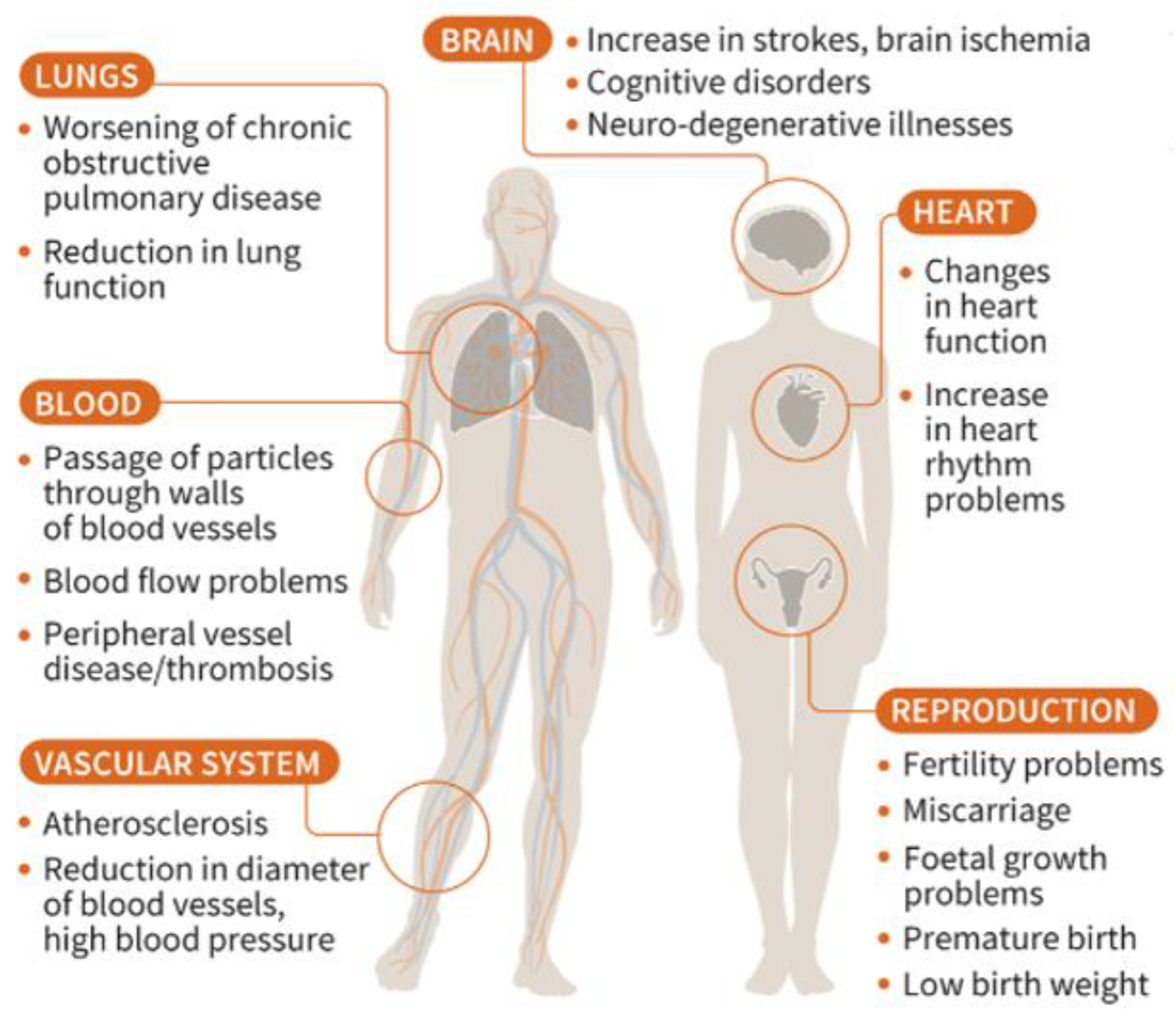
Fine particulate matter (PM2.5) indicates particles with an aerodynamic diameter of 2.5 μm or less. It is not a specific chemical, such as sulfur oxides () and nitrogen oxides (), but a mixture of particles of varying sizes, components, and shapes. Typical substances that form PM2.5 include elemental carbon (EC), organic carbon (OC), , volatile organic compounds (VOC), ozone (), ammonia (), , condensate particles, metal particles, mineral particles, etc. Because of its small size, it penetrates the body through the respiratory tract, causing inflammation or damaging organs [1]. The WHO considers PM2.5 a major environmental risk factor that causes cardiovascular, respiratory, and various other cancers [2]. Figure 1 shows the effects of PM2.5 on the body [3].
Korea’s PM2.5 concentration was the highest among the 37 OECD (Organization for Economic Co-operation and Development) countries in 2019 [4], and studies have shown that it has a negative effect on people’s health. Han et al. [5] stated that 1763 early deaths in Seoul in 2015 were closely related to PM2.5. Hwang et al. [6] explained that, when the average annual concentration of PM2.5 in Seoul increases by , the risk of death over 65 years increases by 13.9%. This is in line with the major causes of death for Koreans in 2019. Statistics Korea shows that cancer (158.2 deaths per 100,000 people), cardiovascular diseases (60.4 deaths per 100,000 people), and pneumonia (45.1 deaths per 100,000 people) are the three major causes of death [7]. This suggests that PM2.5 is highly correlated to the main cause of death for Koreans.
The Korean government is making great efforts to reduce PM2.5 concentration to protect people’s health. The government has divided the crisis into three stages according to the current status and prediction of PM2.5 concentration and has devised a manual for local governments for each stage of action. The government also aims to reduce the annual average concentration of PM2.5 by 35% compared to 2016 by establishing a five-year plan for PM2.5 concentration reduction. To achieve this purpose, the government selected 15 major tasks by evaluating its potential reduction, cost effectiveness, linkage with other policies, and social impact. These tasks are implemented by each local government [8].
Table 1 shows Korea’s crisis stage standard for PM2.5 concentration, which reflects the concentration of PM2.5 in the current period and future forecast values. It suggests that the accurate prediction of PM2.5 concentration is needed in the short and long terms. In this regard, several studies have conducted air quality prediction using deep learning methods with domestic data (wind speed, NO2, SO2, temperature, etc.) in Korea, and new deep learning models have been developed to show high performance in air quality prediction [9,10]. However, foreign factors should also be considered in predicting PM2.5 concentration in Korea, as the concentration of PM2.5 in the Shandong region of China is also found to affect Korea’s PM2.5 concentration [11]. However, as China’s past PM2.5 concentration data are composed of daily data, Korea’s data should also be organized on a daily basis for deep learning PM2.5 prediction. This data composition can cause a “curse of dimensionality” due to the small number of observations compared to variables, which can reduce the performance of the model.
This study aims to show that the application of principal component analysis (PCA) in the deep learning time series prediction models for PM2.5—a recurrent neural network (RNN), long short-term memory (LSTM), and bidirectional LSTM (BiLSTM)—can result in better performance by comparing the root-mean-square error (RMSE) and mean absolute error (MAE) with the same models without PCA application.
2. Previous Research
Several studies have shown the association of PM2.5 with lung and cardiovascular disease (CVD). Wang et al. [12] reported that CVD is the one of the main mortality factors of elder people. It was found that the ambient PM2.5 concentration is related to several CVDs by linking PM2.5 exposure and CVD based on multiple pathophysiological mechanisms. César et al. [13] showed that the exposure to PM2.5 can cause hospitalizations for pneumonia and asthma in children younger than 10 years of age through an ecological study of time series and a generalized additive model of Poisson regression. Kim et al. [14] reported associations of short-term PM2.5 exposure with acute upper respiratory infection and bronchitis among children aged 0–4 years through a difference-in-differences approach generalized to multiple spatial units (regions) and time periods (day) with distributed lag non-linear models. Vinikoor-Imler et al. [15] studied the relationship between PM2.5 concentration, lung cancer incidence, and mortality by linear regression and concluded that there is a possibility of an association between them. Choe et al. [16] reported that the effect of changes in PM2.5 emissions on changes in internal visits and hospitalization probabilities due to respiratory diseases was estimated through Probit and Tobit models. If PM2.5 emissions change by 1%, the probability of visitation due to respiratory diseases increases from 0.755% to 1.216%, and the probability of hospitalization increases from 0.150% to 0.197%.
The need for prediction research is emerging, and various studies are underway on prediction. Zev Ross et al. [17] developed the land use regression model to predict PM2.5 in New York City and showed that urbanization factors such as traffic volume and population density have a high explanation in predicting PM2.5. Rob Beelen et al. [18] compared the performance of ordinary kriging, universal kriging, and regression mapping in developing EU-wide maps of air pollution and showed that universal kriging performs better in mapping , , and . Vikas Singh et al. [19] suggested a cokriging-based approach and interpolated in areas not observed in the network in monitoring based on the suggested method with secondary variable from the results of a deterministic chemical transport model (CTM) simulation. And the results showed that the proposed method provides flexibility in collecting ultrafine dust data.
Other studies have shown examples of predicting PM2.5 through machine learning and deep learning. Zhao et al. [20] predicted the PM2.5 contamination of stations in Beijing using long short-term memory—fully connected (LSTM-FC), LSTM, and an artificial neural network (ANN) with historical air quality data, meteorological data, weather forecast data, and the day of the week data. They showed that the LSTM-FC model outperforms LSTM and the ANN, with MAE = 23.97–50.13 and RMSE = 35.82–69.84 over 48 h. Karimian et al. [21] also predicted Tehran’s PM2.5 concentration by implementing multiple additive regression trees (MARTs), a deep feedforward neural network (DFNN), and a new hybrid model LSTM with meteorological data (temperature, surface-level pressure, relative humidity, etc.). The best model in this research was LSTM in 12, 24, and 48 h prediction, with RMSE = 7.03–11.73 μg/m3 and MAE = 5.59–8.41 μg/m3. Qadeer et al. [22] used XGBoost (XGB), the light gradient boosting machine (LGBM), the gated recurrent unit (GRU), convolutional neural network–LSTM (CNNLSTM), BiLSTM, and LSTM to predict PM2.5 concentration of eight sites in Seoul and Gwangju with community multiscale air quality (CMAQ) data. The result showed that LSTM performs best, with MAE = 3.5847 μg/m3, RMSE = 4.8292 μg/m3, R = 0.8989, and IA = 0.9368 of the mean in all sites.
The RNN, LSTM, and BiLSTM models were used in this study, because previous studies have shown that the deep learning sequence model performs better in prediction. The local weather and air quality data were used to predict PM2.5, as shown in previous studies, and used as predictive input variables. The regional data of China are also used as predictive input variables, which were found to affect PM2.5 in Korea.
3. Data
3.1. Spatial Area
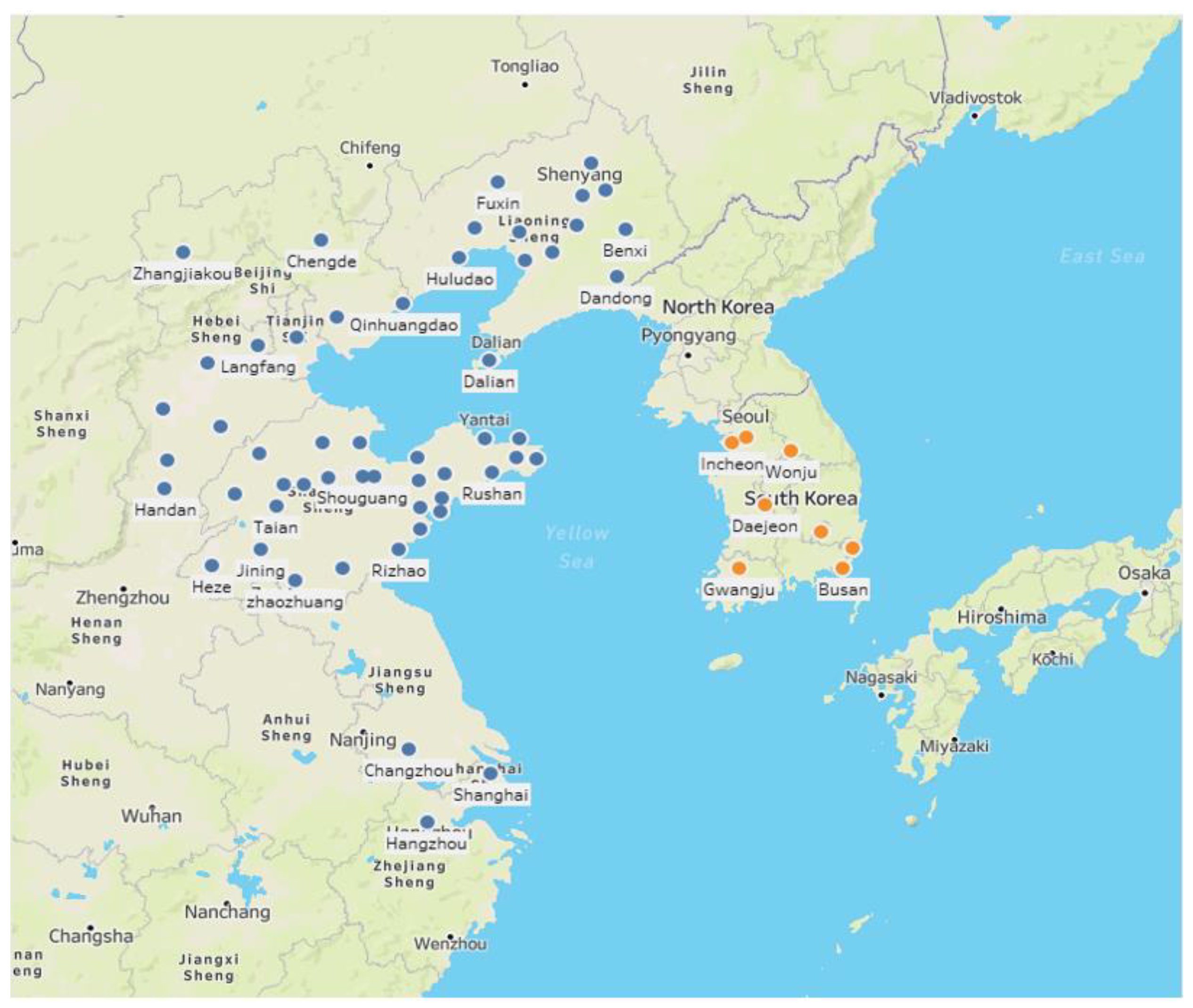
Figure 2 shows the spatial range of the research. A total of eight cities in Korea were selected for analysis. Of the eight cities, six are metropolitan cities (Busan, Daejeon, Daegu, Gwangju, Incheon, and Ulsan) representing each province, one is the capital city (Seoul), and one is the most populous city (Wonju) in the province without a metropolitan city. In each city, daily air quality data (PM2.5, SO2, O3, NO2, and CO) [23] and meteorological data (temperature, wind speed, wind direction, humidity, precipitation, etc.) [24] were collected in consideration of the internal factors of PM2.5 generation. Air quality data were collected within 5 km of each city’s meteorological data observatory.
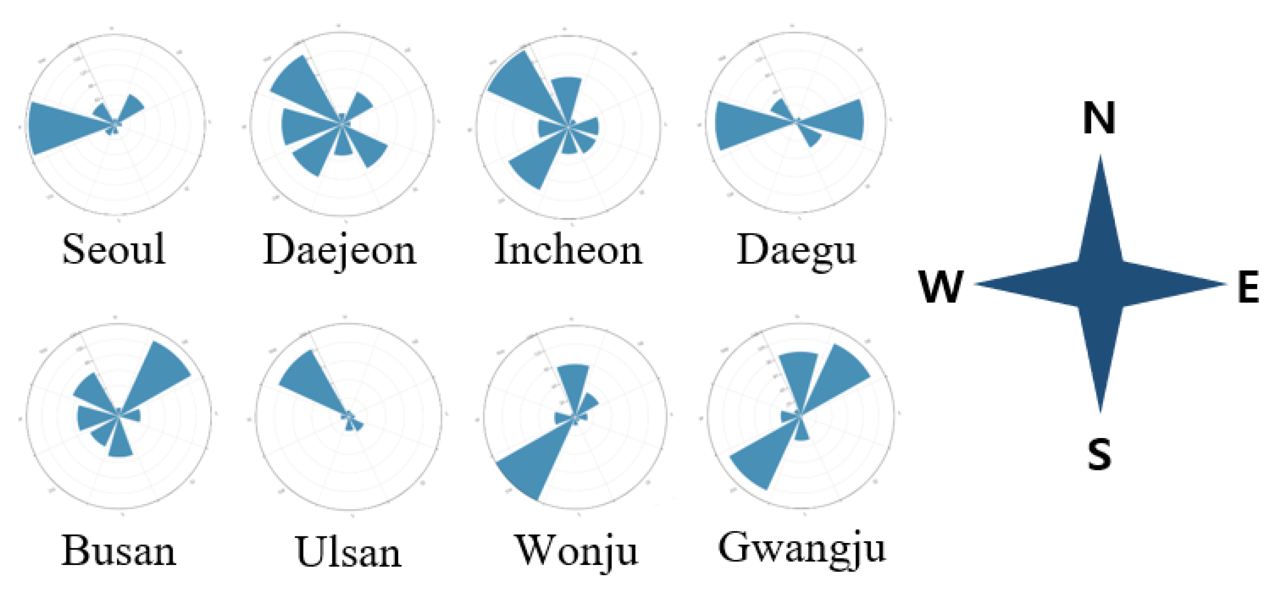
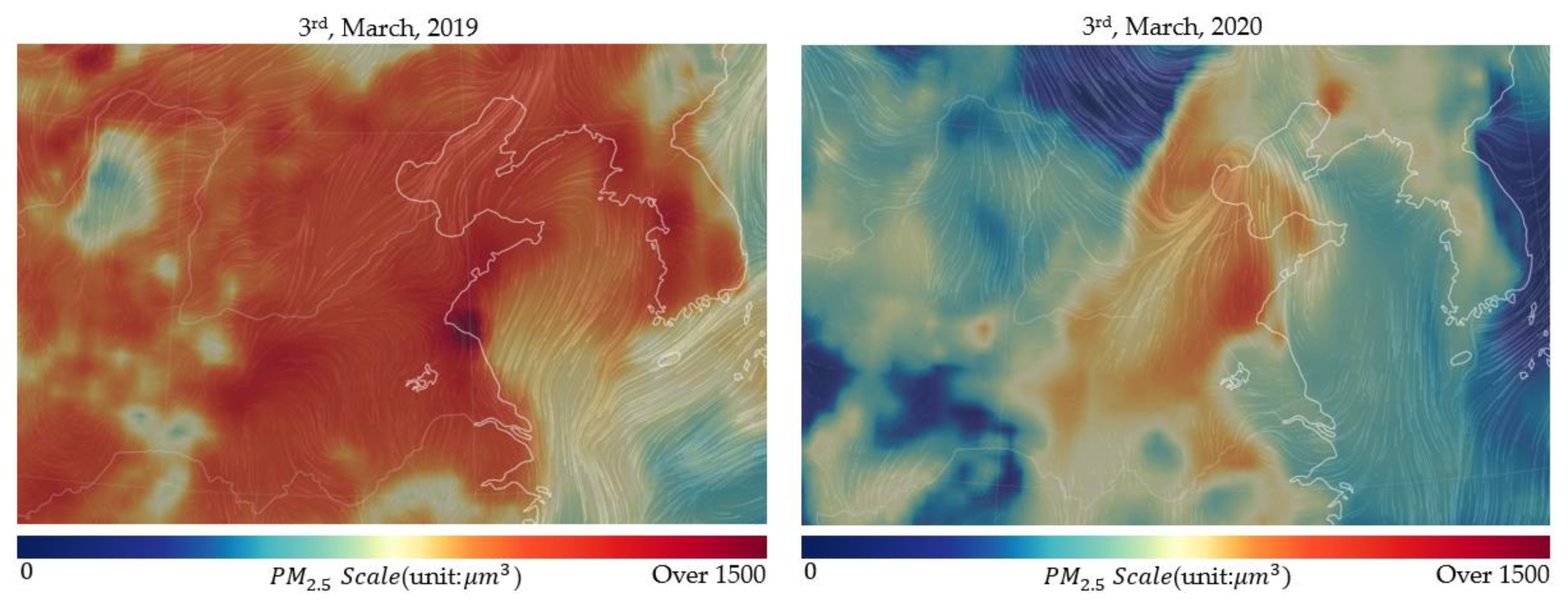
Figure 3 shows that Korea is mainly a country with north and west winds. As a result, the air quality of Korea can be directly and indirectly affected by the air quality of China, a country located in the west and north. Figure 4 [25] also shows the concentration of PM2.5 in Korea and China at the same time before and after the outbreak of COVID-19. According to Bao et al. [26], it can be seen that the lockdown of Chinese factories after the COVID-19 outbreak actually improved the Chinese air quality. Considering this, with the direction of the wind in Korea, we can see that the air quality of Korea is highly affected by the air quality in China. Accordingly, daily PM2.5 concentrations in 55 areas in China close to Korea were selected as input variables in this study, including the PM2.5 concentration in Shandong province, which was found to increase PM2.5 concentration in Korea.
3.2. Data Preprocessing
All variables have a time range from 1 January 2015 to 31 December 2019 and are collected as daily data. There are missing values in some variables, and these missing values were processed by the exponentially weighted moving average (EWMA) using the imputeTS package of the R software [27]. The EWMA gives higher weights to the latest data, reducing the weight of older values, and the formula for EWMA imputation suggested by Hunter [28] is as follows:
is the predicted value at time t, is the observed value at time t, is the observed error at time t, and is a constant value called the weight from zero to one. The higher the value is, the less it reflects past data.
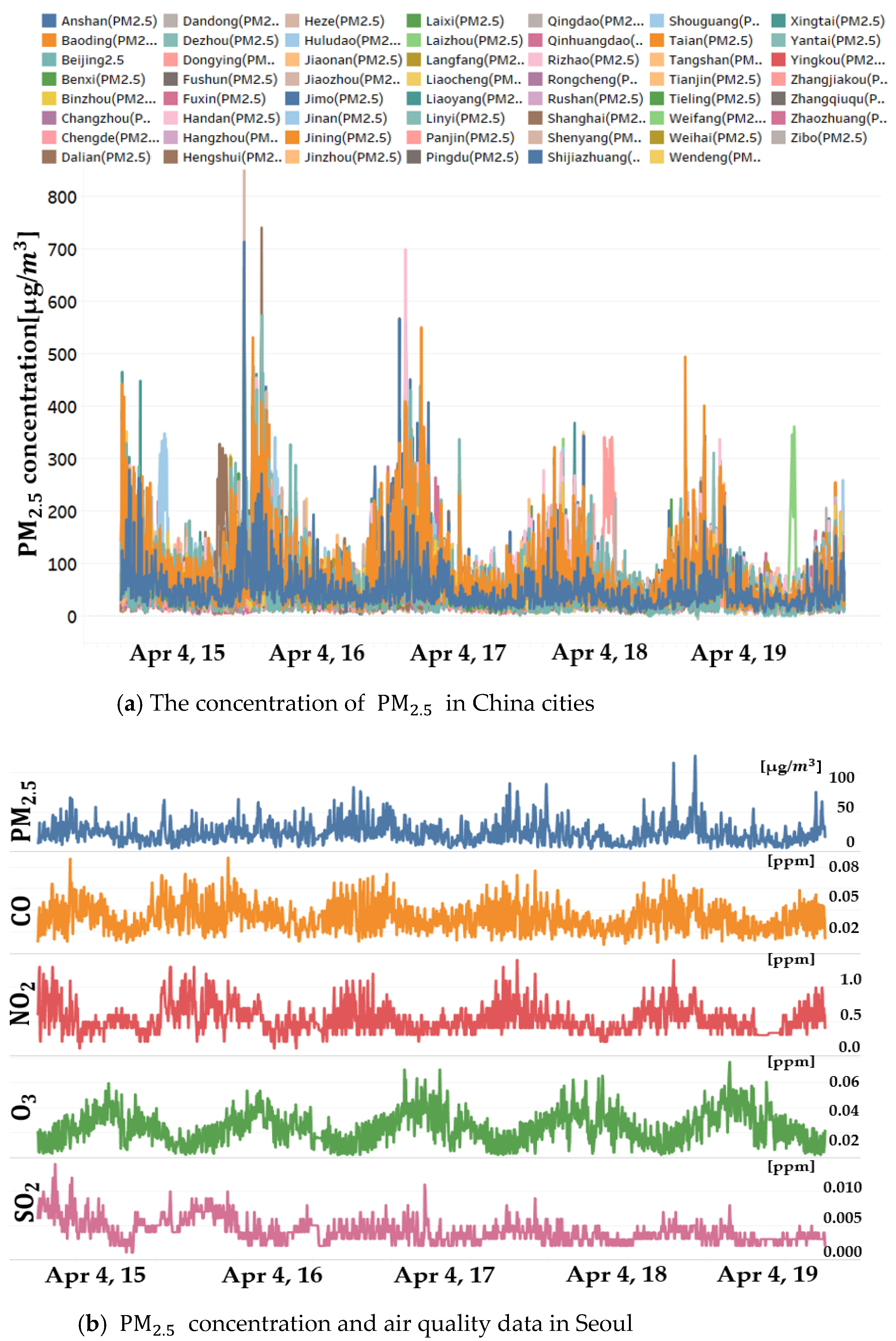
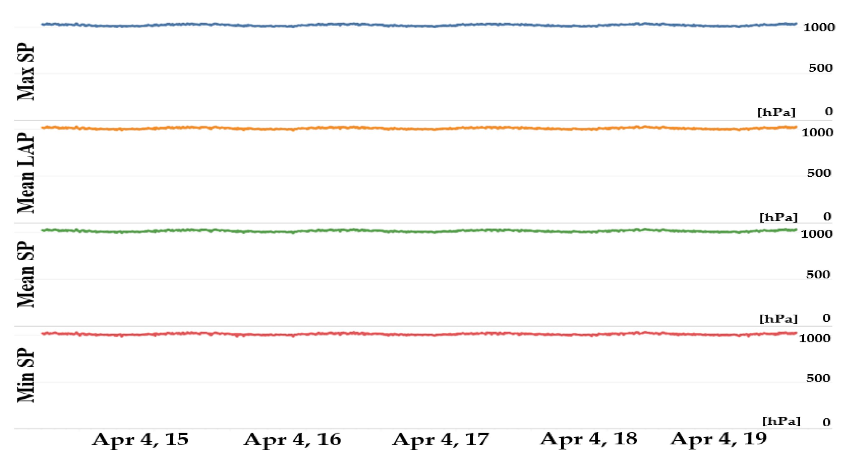
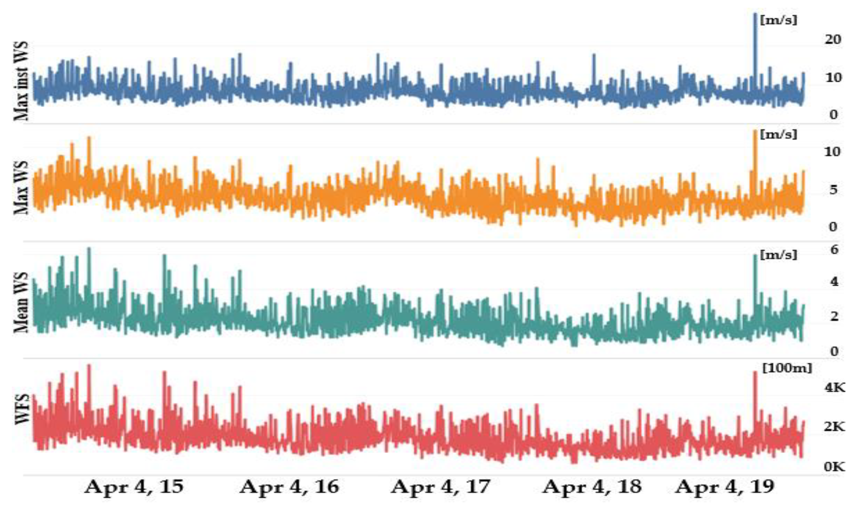
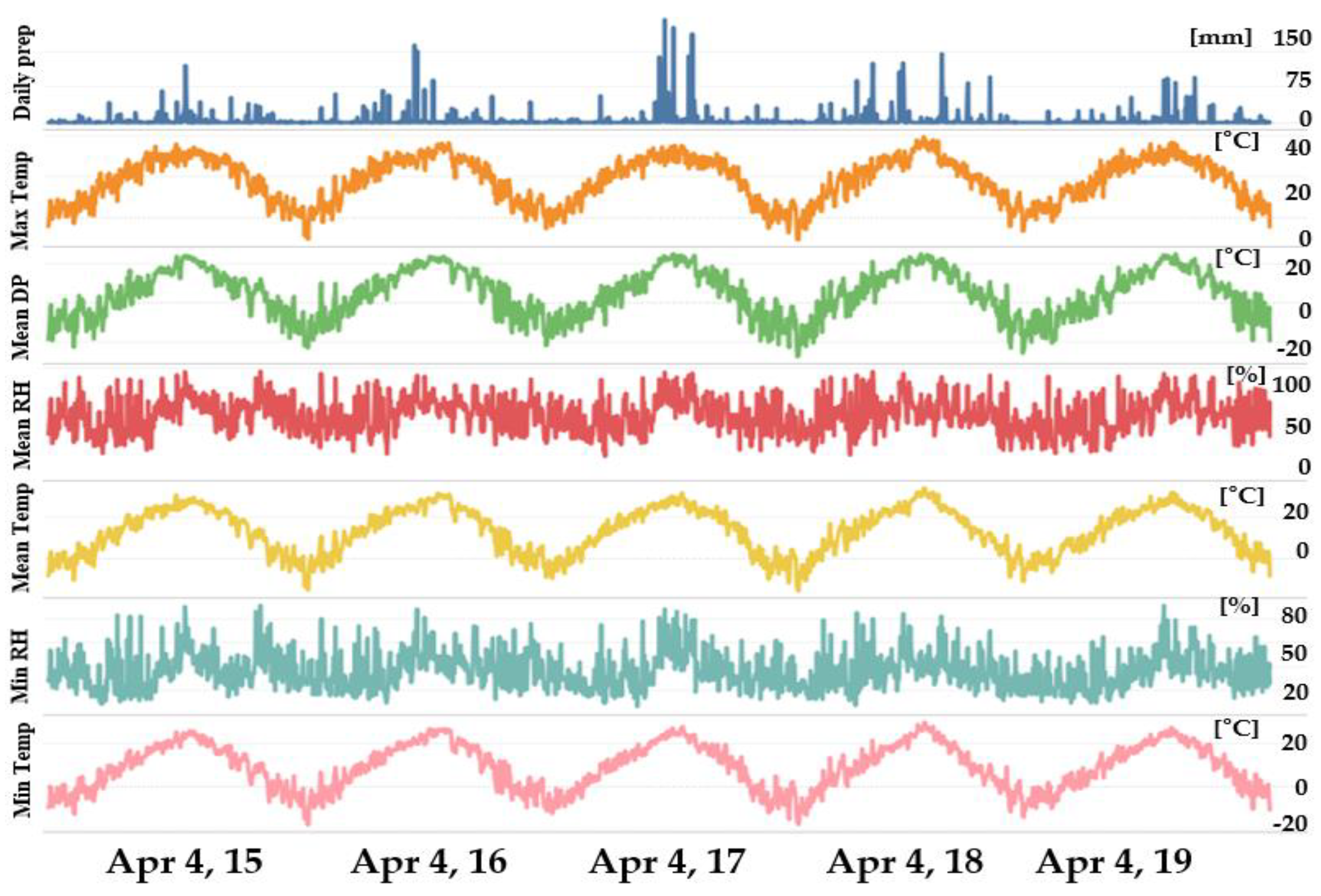
Figure 5 and Figure A1, Figure A2 and Figure A3 show the concentration of PM2.5 in China (Figure 5a), Seoul (Figure 5b) with air quality, and the meteorological data of Seoul (Figure A1, Figure A2 and Figure A3). Each variable shows the values in a different range due to the differences in units of measurement and the characteristics within the region. In the case of Chinese data, the concentration of PM2.5 in each city over time seems to be constant, but some cities have outliers. If one variable has a relatively greater value, or a wider range of values than the others, in the composition of the data, it can result in a significant impact on the predicted value, regardless of the predictive importance of the variable.
To solve these problems, the scope of the variables should be adjusted through normalization. In this study, maximum–minimum normalization was carried out to every data of each city as shown in the following equation:
Because the wind direction data were collected as 16 cardinal points, these are labels encoded to transform direction data into numerical data.
3.3. Variable Correlation Analysis
As mentioned above, the prediction target of this study is the concentration of PM2.5. The efficiency of the forecast results in deep learning, and machine learning depends on the correlation between the dependent and the independent variables. It is important to add variables with a strong negative or positive correlation between the dependent variable and the independent variable. In addition, the results of correlation are necessary for data analysis because they provide a basis for determining the influence of each independent variable on a dependent variable. In this study, the Pearson correlation coefficient was calculated, which is expressed as the covariance and standard deviation of the variables, as shown in the following equations in the case of observation vector :
Each element in the correlation matrix has a value between −1 and 1, showing that a value greater than 0 is a positive correlation and a value less than 0 is a negative correlation. The correlation matrix is symmetric, and all of the diagonal elements of the matrix have a value of 1 considering , .
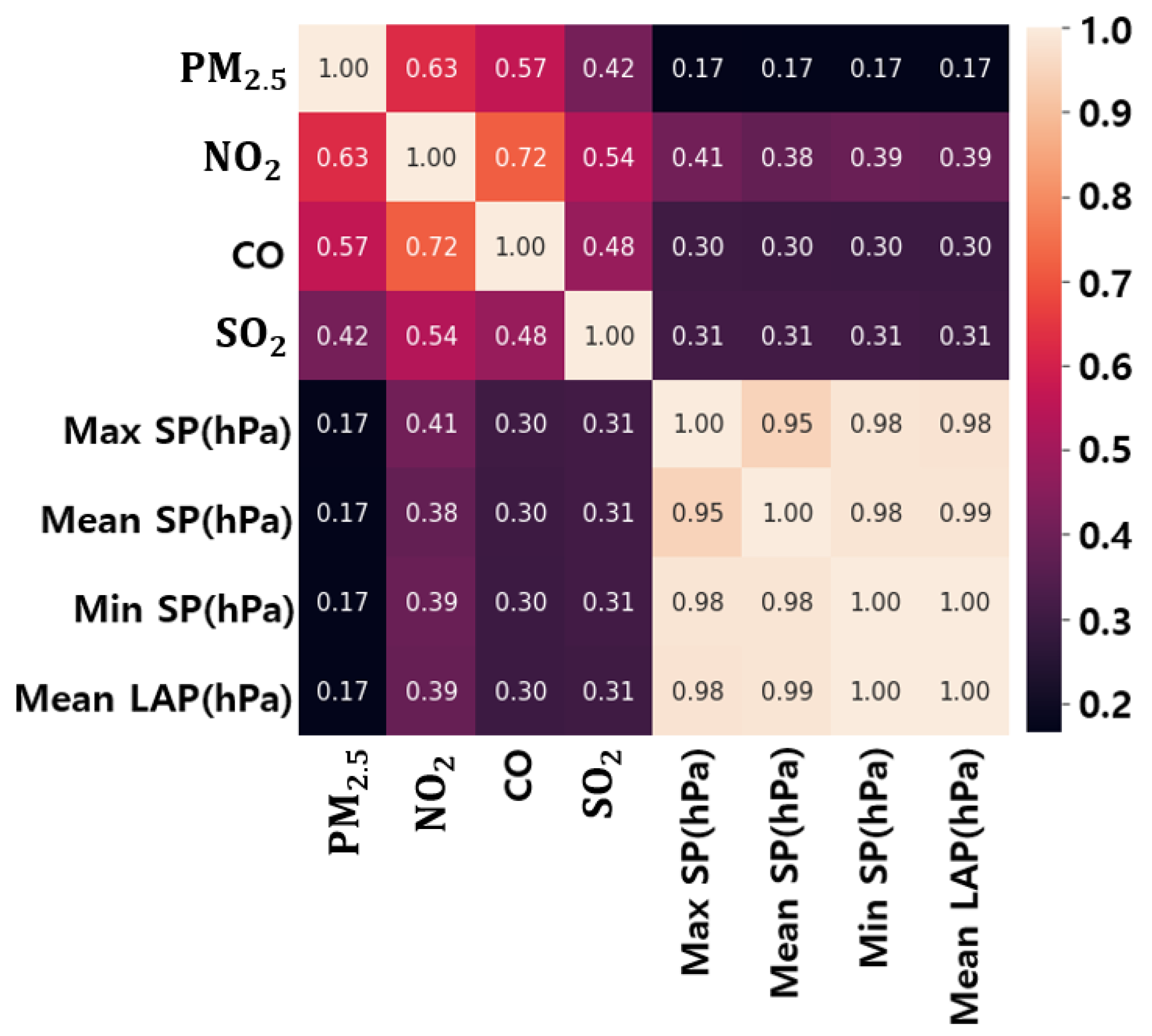
Figure 6 is a visualization of the correlation between concentrations and the highest eight factors inside Seoul, Korea. Appendix A Table A2, Table A3, Table A4, Table A5, Table A6, Table A7, Table A8 and Table A9 show the correlation between PM2.5 concentrations and the meteorological air quality factors of each city in Korea. Overall, the factors that have a strong positive correlation with PM2.5 are air quality factors except for O3. PM2.5 also appears to have a positive correlation with local air pressure (LAP), sea-level pressure (SP), wind direction, and relative humidity. Conversely, temperature, wind speed, O3, wind flow sum (wind flow sum refers to the distance that the air flows, and the Korea Meteorological Administration produces a day-to-day wind flow sum (24 h wind flow sum).), and daily precipitation were found to have a negative correlation with PM2.5 concentrations. However, the variables that have a relatively weak correlation with PM2.5 changed the sign of the correlation depending on the region.
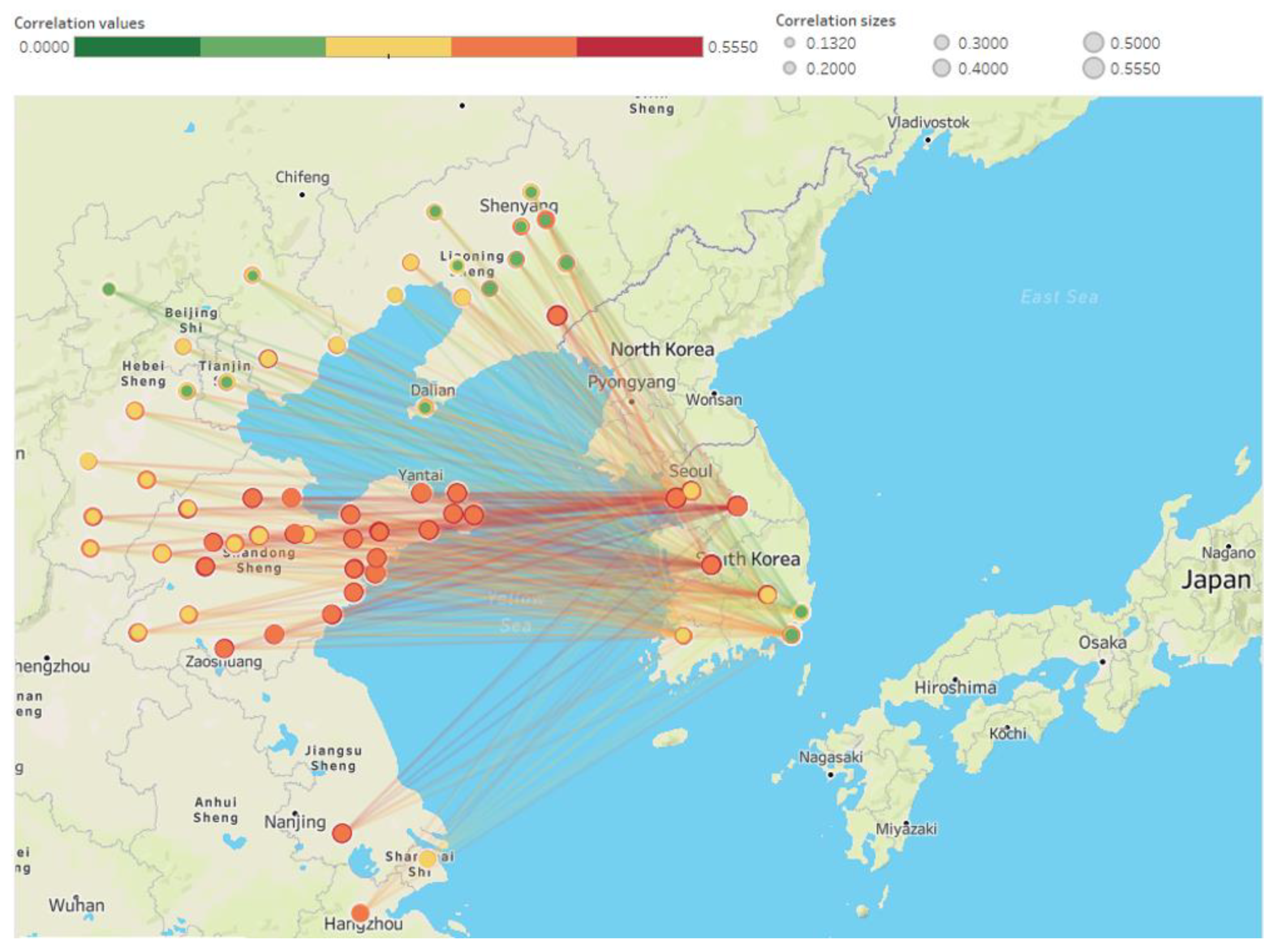
Figure 7 shows an origin–destination map of PM2.5 correlations between Chinese [29] and Korean cities. The correlations between PM2.5 concentrations in each Chinese city and PM2.5 concentrations in each Korean city vary, but as shown in Table 2, an overall correlation between 0.13 and 0.55 is shown. Comparing this with the factors inside the Korean cities, we can see that the PM2.5 concentration of each city in China is as much related with the PM2.5 concentration in Korea as the data of air quality inside the city. This suggests that China’s PM2.5 concentration could be an important independent variable in predicting PM2.5 concentrations in Korea.
4. Analytical Methods
4.1. PCA
PCA reduces dimensions by linear combinations of variables with high explanatory power of the overall data variability, explaining variation in high-dimension data in low dimensions. Vectors with p variables can have total p principal components, and the principal components of vector , whose covariance matrix is , can be generated as follows:
Because the principal component is a linear combination of , it can be expressed as Equation (9), and the variance of this linear combination can be expressed as Equation (10). The PCA has to preserve the variance of the original data as much as possible, so Equation (10) should also be maximized. Therefore, the method of generating principal components can be transformed into the problem of obtaining , which maximizes under the condition . Equation (11) was derived by applying Lagrange’s multiplier method to Equation (10). Equation (13) was made by Equation (12), which partially differentiates Equation (11) by . Equation (13) shows that is the eigenvalue of , and is the eigenvector of . As a result, a linear combination that maximizes Equation (10), i.e., the principal component, can be expressed as Equation (9). In addition, Equation (10), which is the variance of the principal component, can be expressed as under the condition . Therefore, in vectors with p variables, the i-th principal component is Equation (15), and the variance is Equation (16). Subsequently, the number of principal components is selected for convenience by the principal components where the sum of the principal components is more than 80% to 90% of the total variance. For example, the number of principal components i has to be selected out of principal components p. Equation (17) has to produce results of more than 80% to 90%:
4.2. RNN
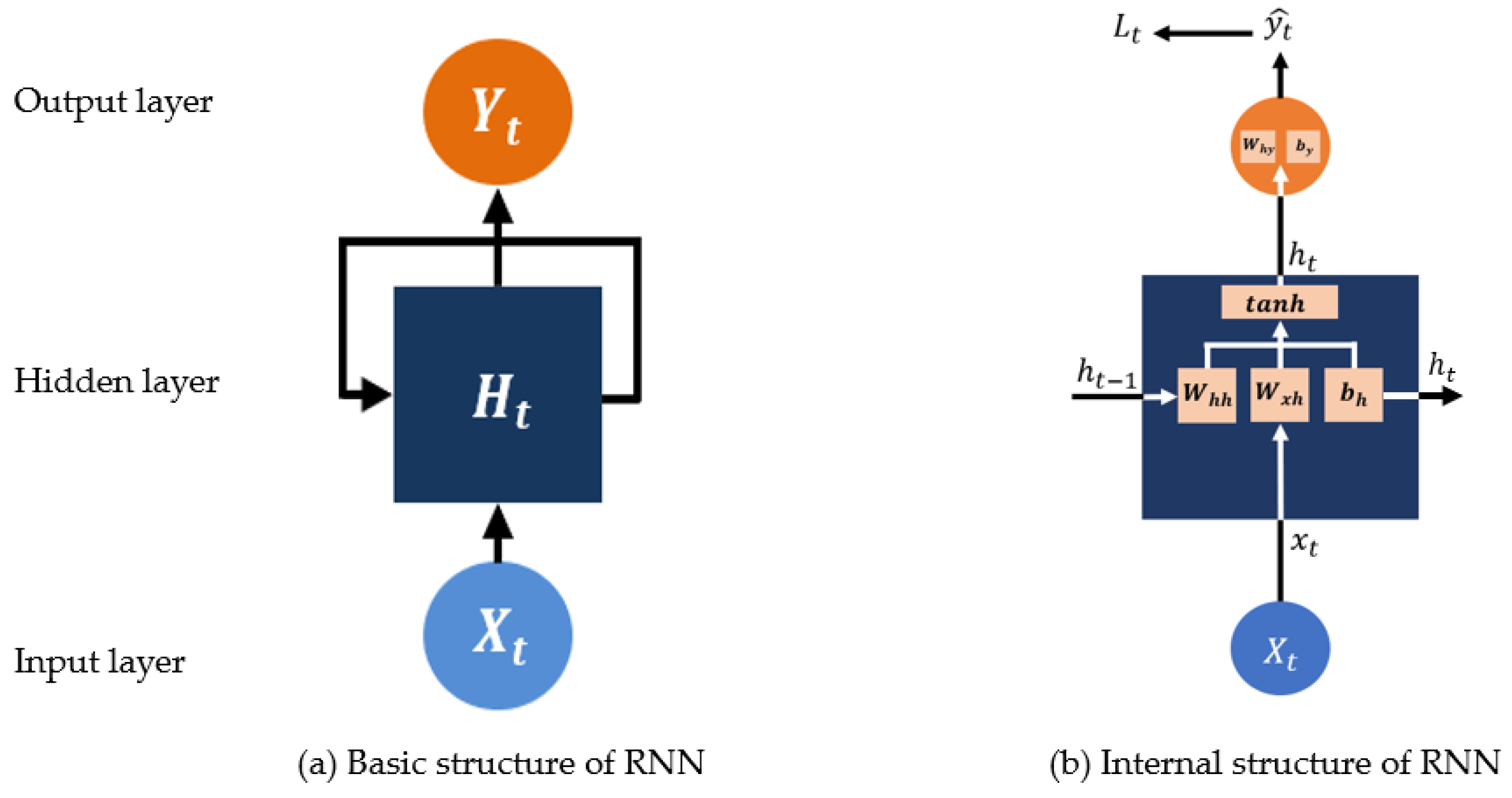
The RNN is a deep learning model for processing sequence data, such as stock charts [30], music [31], and natural language processes [32]. It remembers the state entered from the previous time point (t − 1) through the hidden layer and passes the hidden layer state at that specific time point (t) to the next time point (t + 1). That is, the status at the previous time point affects the state at the present time point, and the state at the present time point affects the status at the next time point. This procedure is repeated until result values becomes optimized; hence the name “recurrent neural network.”
Figure 8b is the unrolled and inner structure of Figure 8a. In Equations (18)–(20), is an input, and is a hidden state at time t. is the weight from layer i to layer j, and is the bias in each layer. In Equation (21), is the loss at time t, and and are the actual and predicted values, respectively, at time point t.
The RNN model shares the weights and biases at all time points and circulates the input data to output the results. Model training is repeated until the loss value is minimized by gradient descending in the loss function, with information of specific previous time steps. At the same time, the weight is updated to find the optimum value. This is called backpropagation through time (BPTT) and in an RNN can be expressed as follows [33]:
4.3. LSTM and BiLSTM
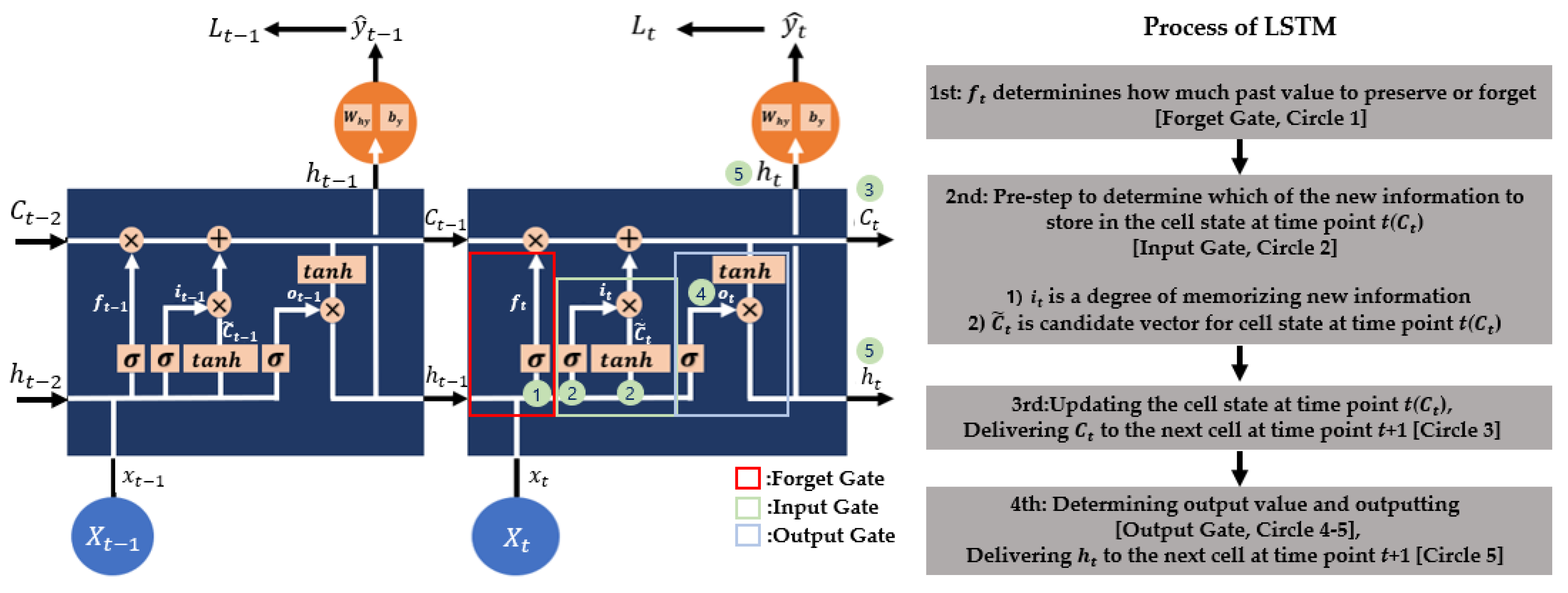
In an RNN, tanh is used as an activation function to train the model in a non-linear way. However, there is a long-term dependency problem caused by a “vanishing gradient” problem in the RNN’s BPTT, in which the gradient (weights update rate) disappears as the value (derivative value of the tanh function with respect to ) less than 1 continues to multiply. Thus, the state of a relatively distant past time point has almost no effect on an output of the present time point. As a result, the model relies only on short-term data and has a limit in achieving the best performance. To solve this problem, Hochreiter et al. [34] suggested the LSTM model. Figure 9 shows the internal structure of LSTM and its process.
LSTM is the model in which forgetting and memory (), the input (), the inner cell state candidate , the conveying and inner cell state at time point t (), and the output () are added to the RNN model. Especially, , which penetrates all time points, greatly contributes to solving the long-term dependency problem. The order of each part and the internal algorithm can be explained by the following process:
Equation (25), output of the forget gate, determines whether the historical state is forgotten by the combination of and . The output value of this step is converted to a number between 0 and 1 by the sigmoid function and multiplied by (memory of past data, i.e., historical state) to determine how much past data to preserve or forget. A value of 0 indicates forgetfulness, and 1 indicates memorization of past data. Equations (26) and (27) are involved in the storage of the inner cell state of time point t. Equation (26), output of the input gate, determines how much data of time point t are memorized. In other words, it has a value between 0 and 1, indicating the degree of memorizing for the new information. At the same time, Equation (27) generates the inner cell state candidate of time point t. Equation (28) generates the new cell state at time point t and passes it on to the LSTM cell at the next time point (t + 1). In other words, LSTM solves the RNN’s long-term dependency problem by adjusting the memorization and forgetfulness of the past and presents the state through Equations (25)–(28). In the end, the output is decided by Equations (29) and (30). Equation (29), output of the output gate, decides which part of the new cell state will become output. A value of the new cell status is converted through the tangent function and calculated with the result value of Equation (29) to produce the final output of time point t, as shown in Equation (30).
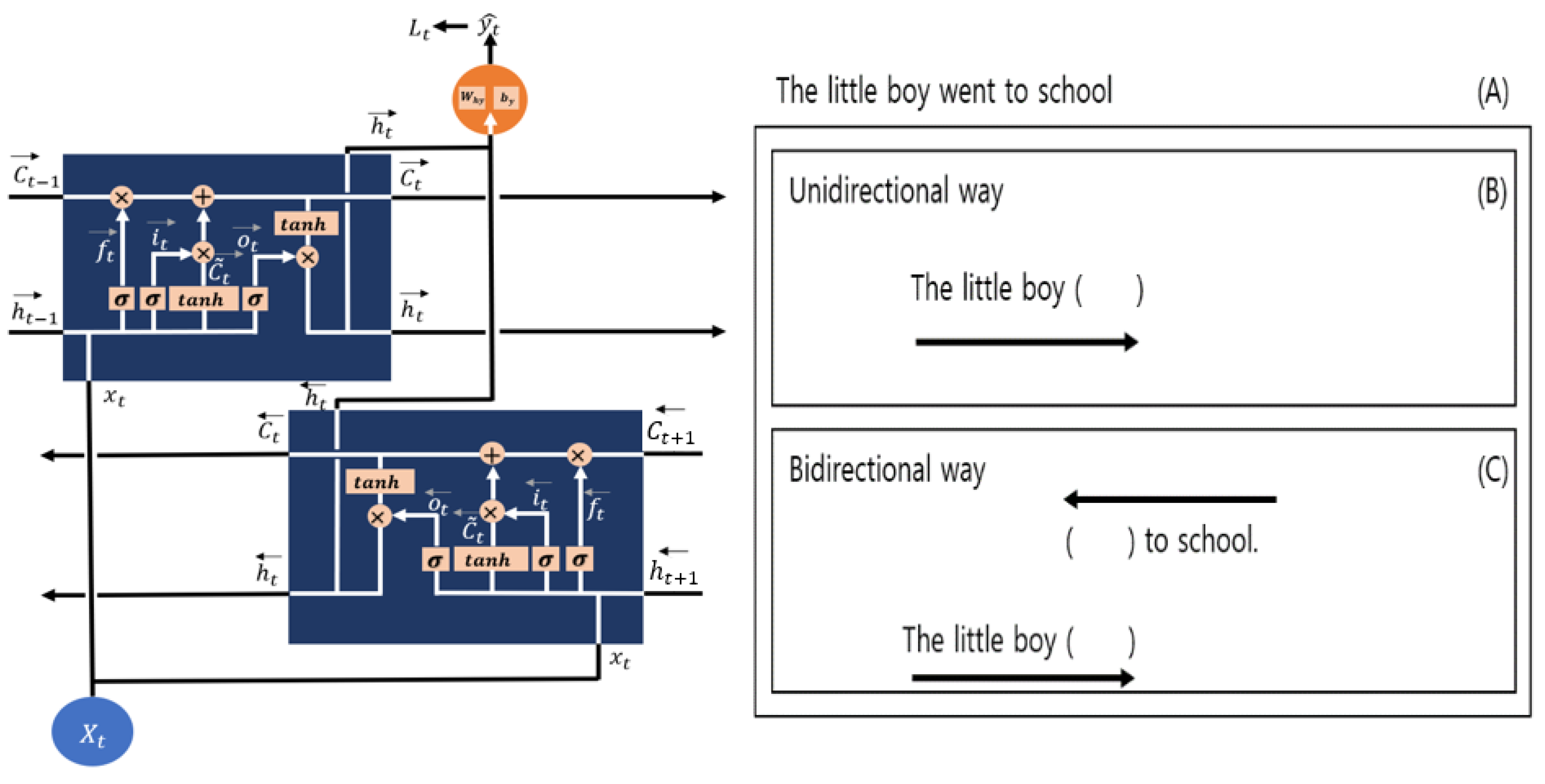
BiLSTM is a variant of the bidirectional RNN proposed by Schuster et al. [35]. Figure 10 shows an example of applying a bidirectional way to sentence learning. If (A) is taught in the model and “went” is set as the target, (B) predicts in a forward way and (C) predicts in both a forward and a backward way. If LSTM uses a historical state to predict the value of time point t, bidirectional LSTM predicts the value of time point t by adding an LSTM layer that reads data from a future state. The computations within the model are the same as those of LSTM, and LSTM and BiLSTM update their weights in the training model as an RNN [36].
4.4. Evaluation Model Performance
In this study, MAE (Mean Absolute Error) and RMSE (Root Mean Square Error) were used as evaluation indicators to compare the performance of each model with and without PCA application. The calculations of each indicator are expressed as follows:
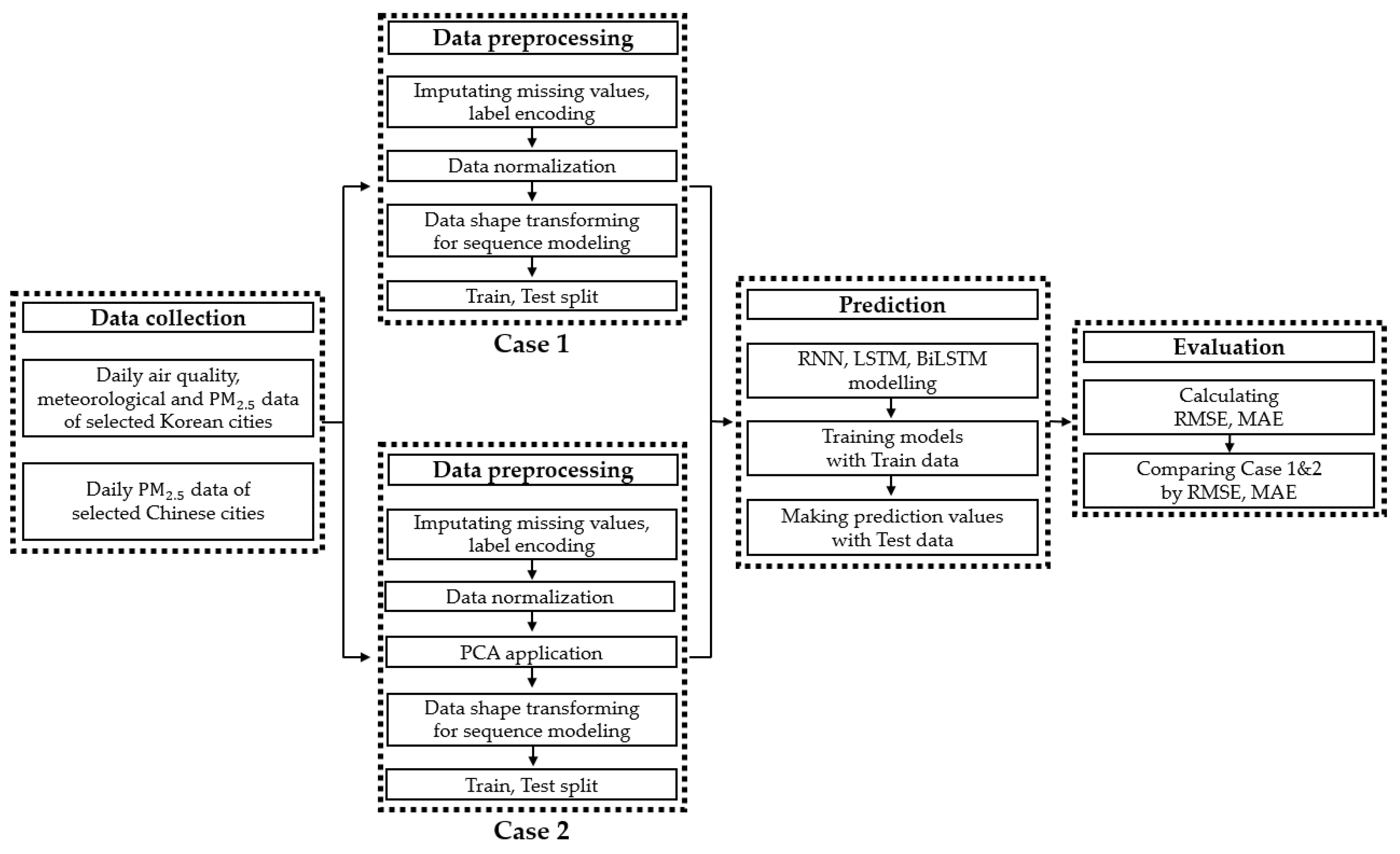
4.5. Workflow
The flow of this study is divided into four stages: data collection, data preprocessing, prediction, and evaluation (Figure 11). The application of PCA is used in the data preprocessing stage, aiming to reduce the number of variables and increase the performance of model predictions. Thus, the data preprocessing stage was divided into two cases. Case 1 was set as a prediction without a PCA application, and Case 2 was set as a prediction with the PCA application. Afterwards, each case will be compared using evaluation indicators (MAE and RMSE).
5. Results
5.1. PC Selection
For each city, PCA was performed on the input variables, except the dependent variable, PM2.5. The variance of each city’s data was explained by a relatively small number of principal components, which resulted in the selection of five principal components in all cities. This reduced the number of input variables to about 1/16. Table A10, Table A11, Table A12, Table A13, Table A14, Table A15, Table A16 and Table A17 show the results of the PCA of each city, and Table 3 shows how much the five principal components describe the overall variation of each city.
5.2. Setup and Case Comparison
China’s daily PM2.5 concentration and Korea’s air quality and meteorological data were collected from 1 January 2015 to 31 December 2019 to predict the concentration of PM2.5 in eight Korean cities. In total, 85% of the collected data were allocated to the train set and 15% to the test set. In the aspect of details in models, the three models have 256 units in the layer, a tanh activation function, 200 epochs, a batch size of 64 and an adaptive moment estimation (ADAM) optimizer [37]. To avoid overfitting, 30% of the train set was designated as a validation set, and a 30% dropout regulation was used between the input layer and the output layer. Additionally, in model learning, earlystopping, one of the callback functions of Keras, was applied to stop learning in the epoch when optimal learning had achieved 200 epochs.
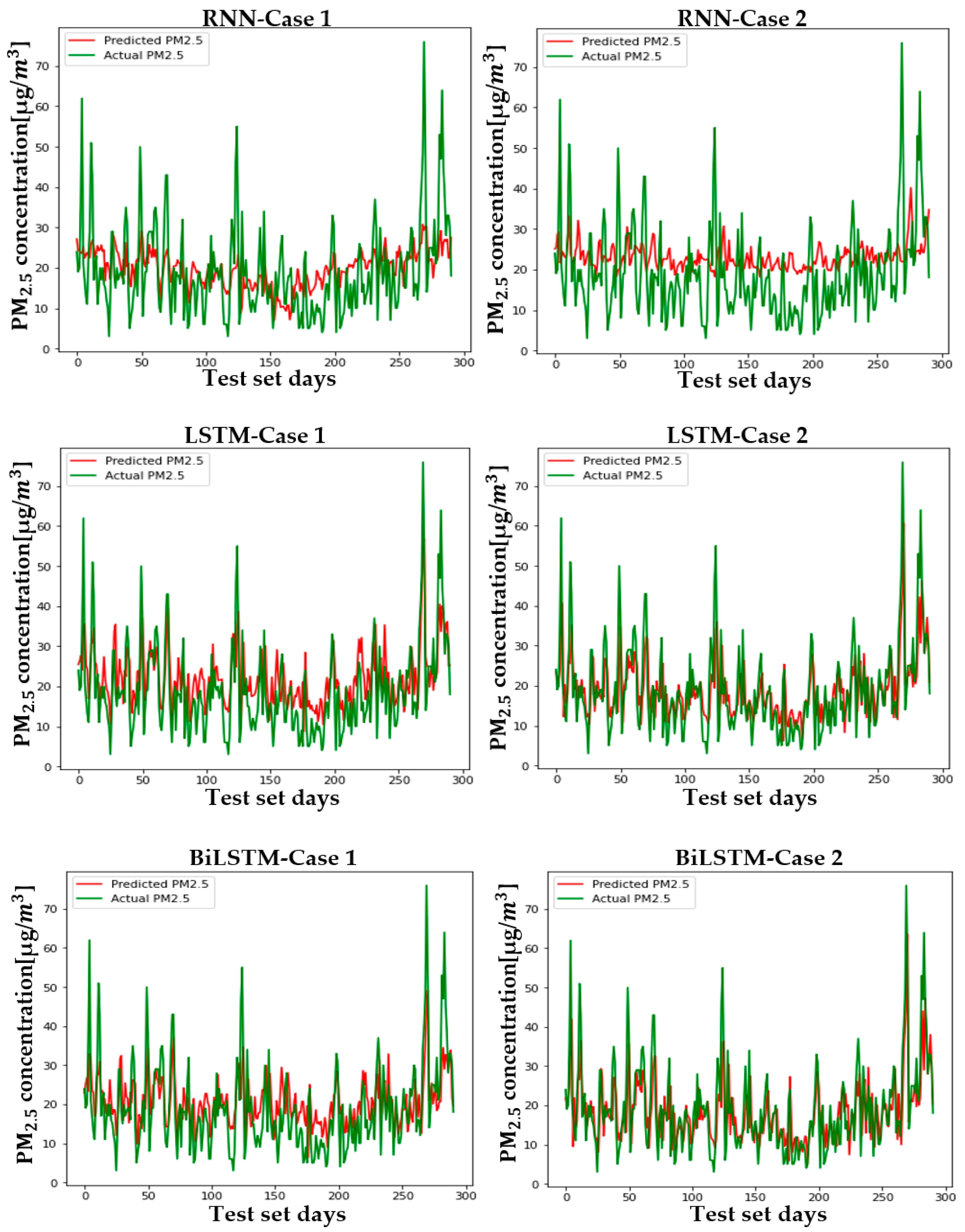
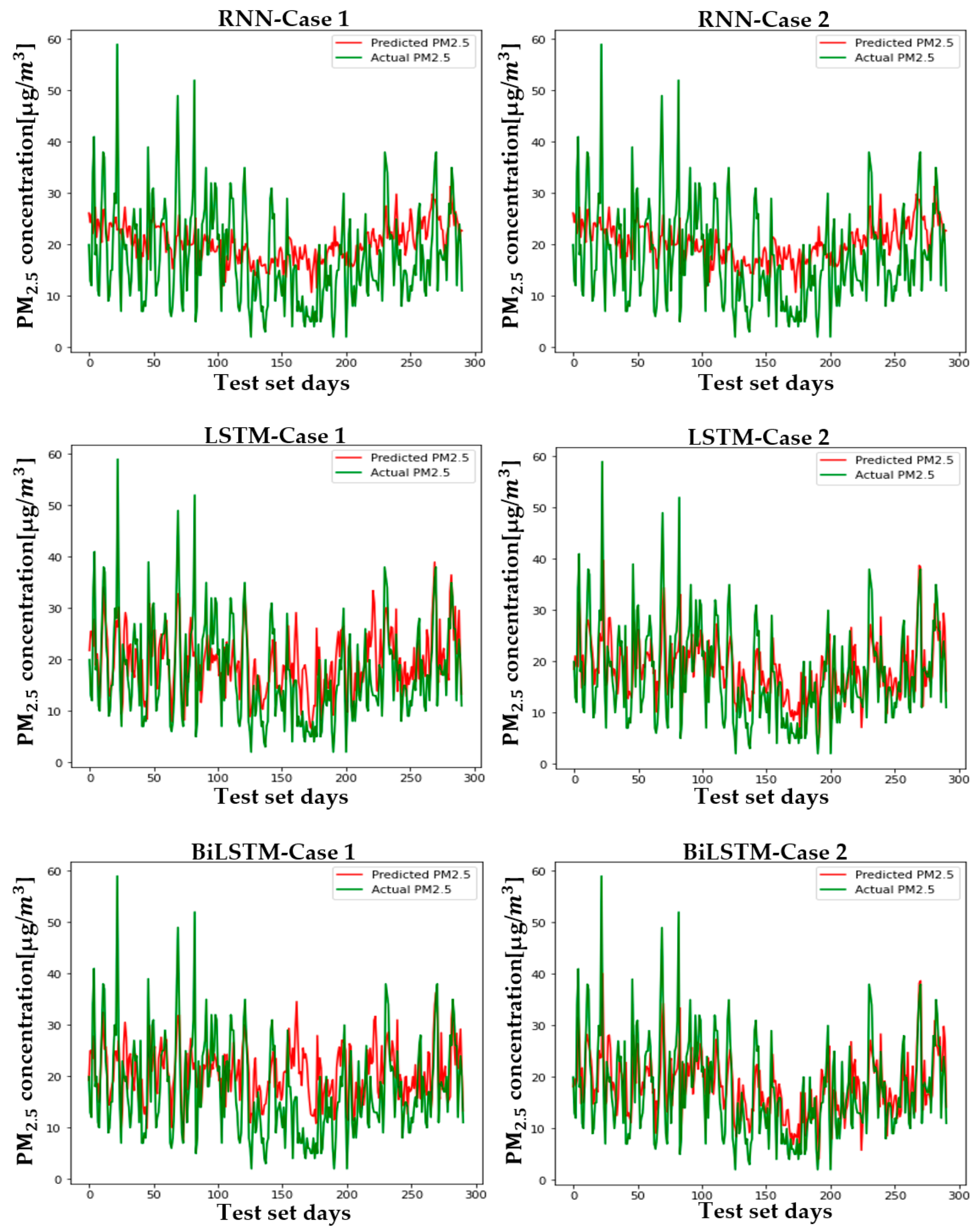
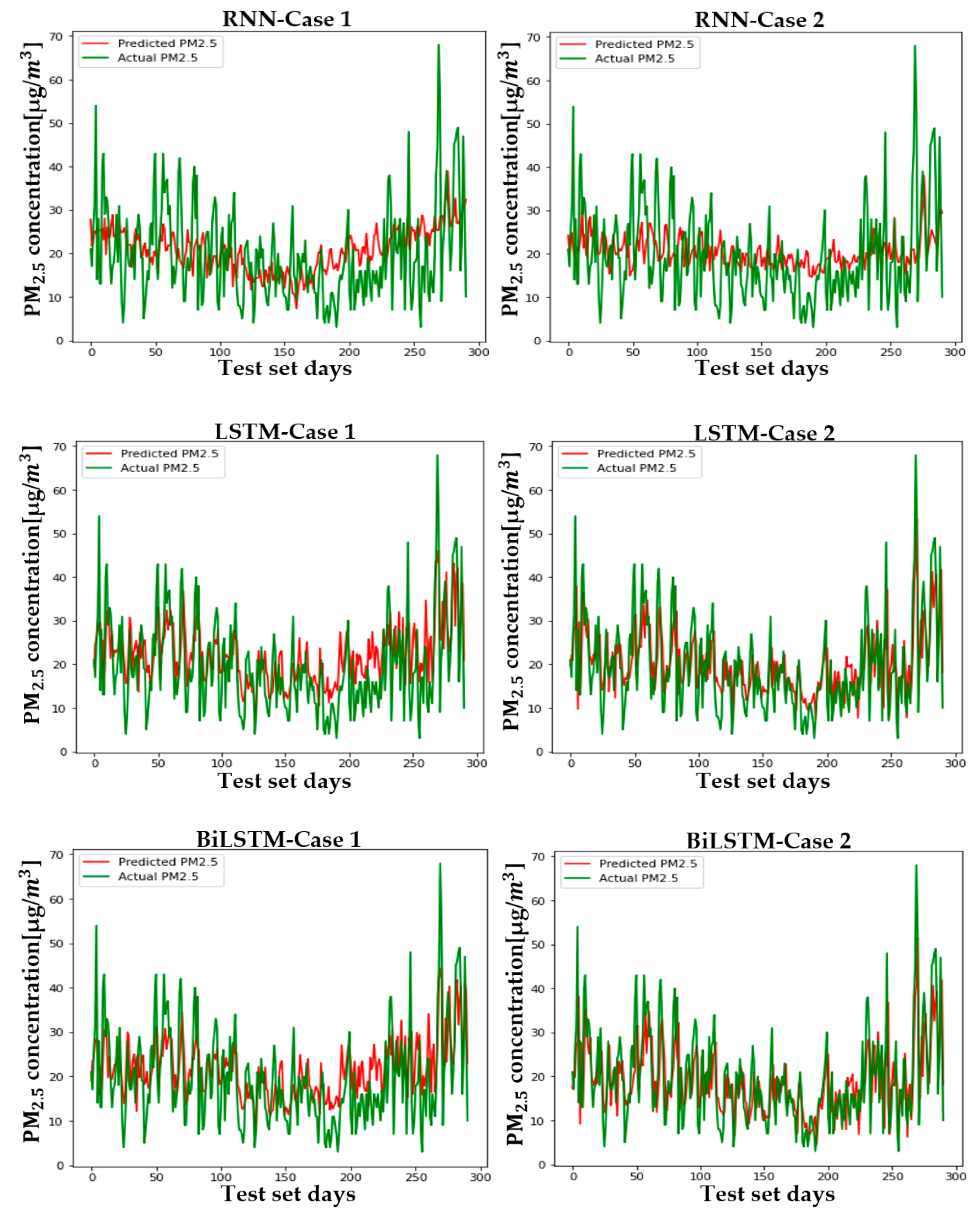
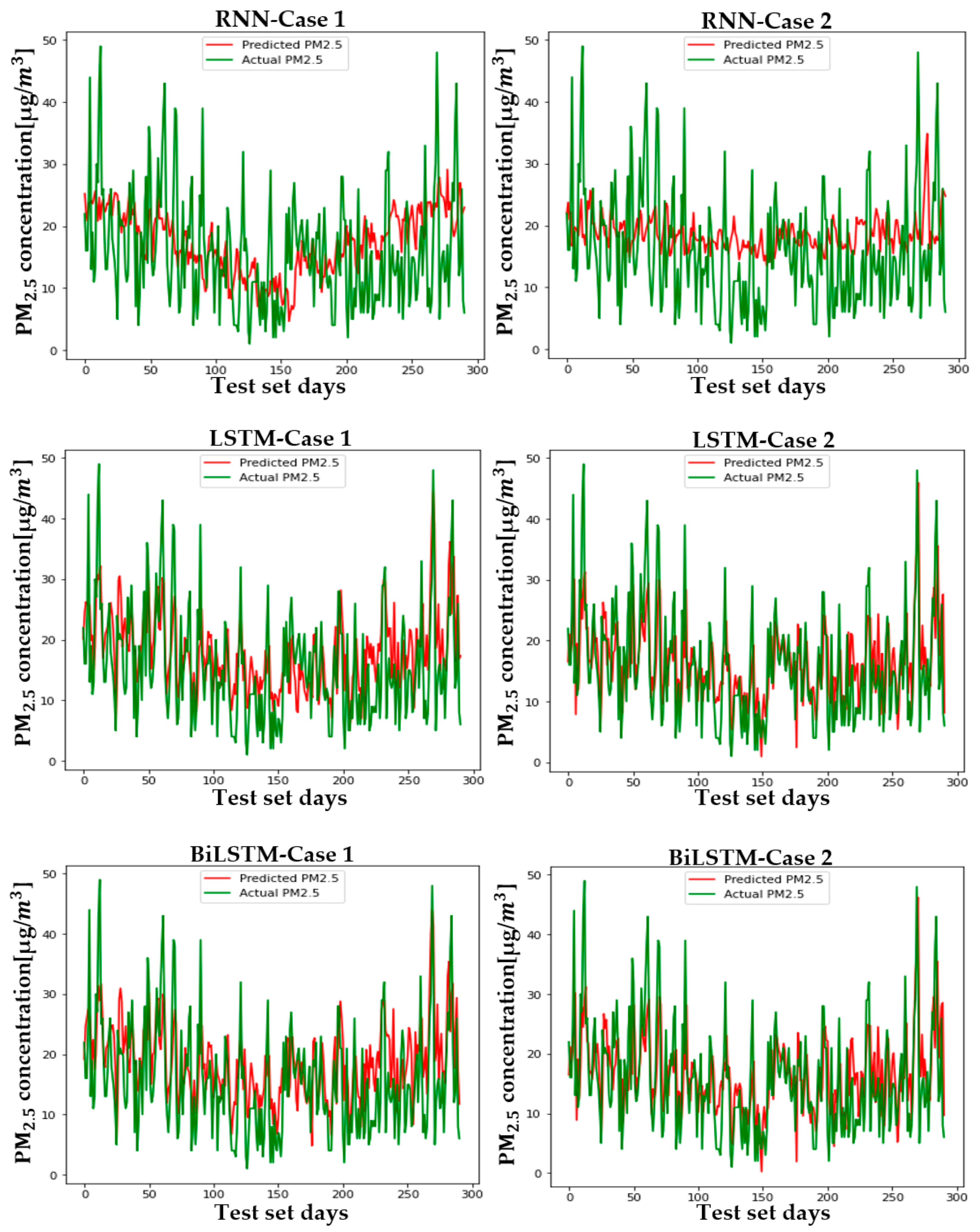
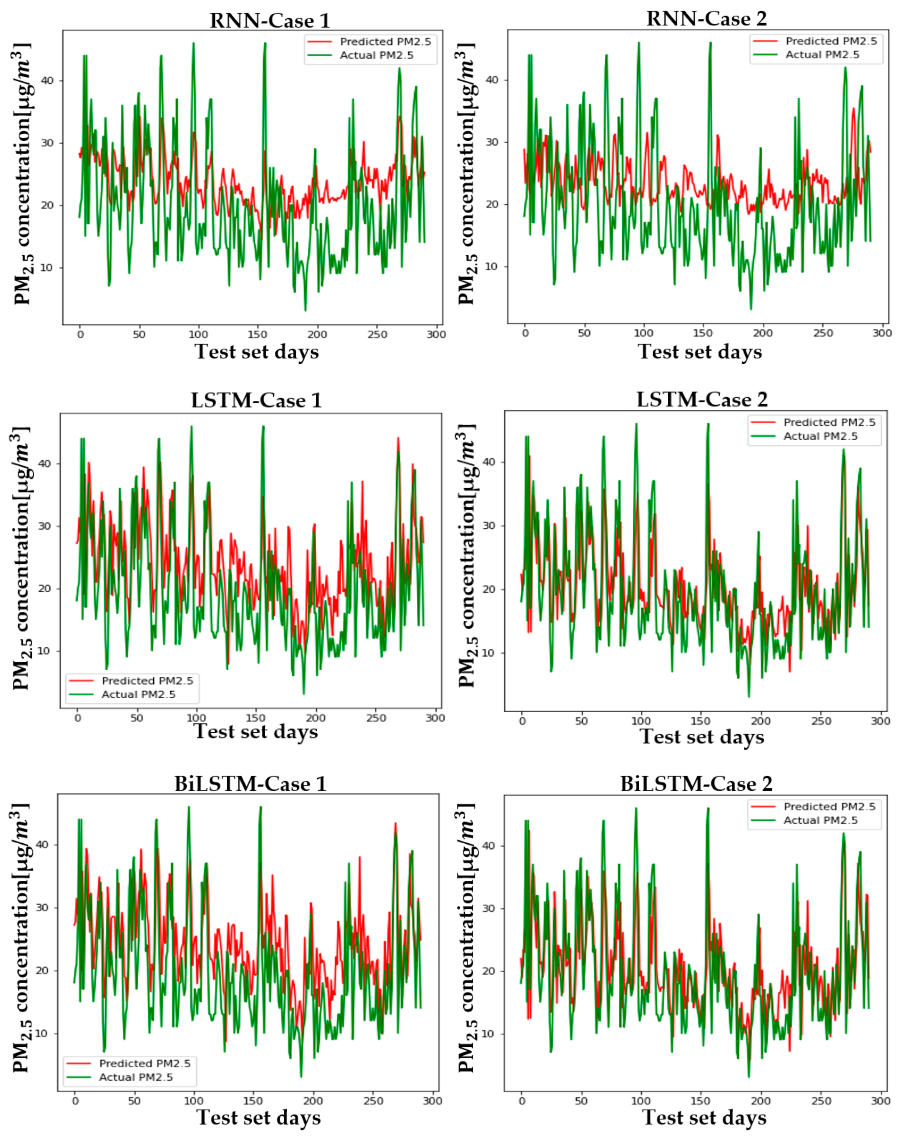
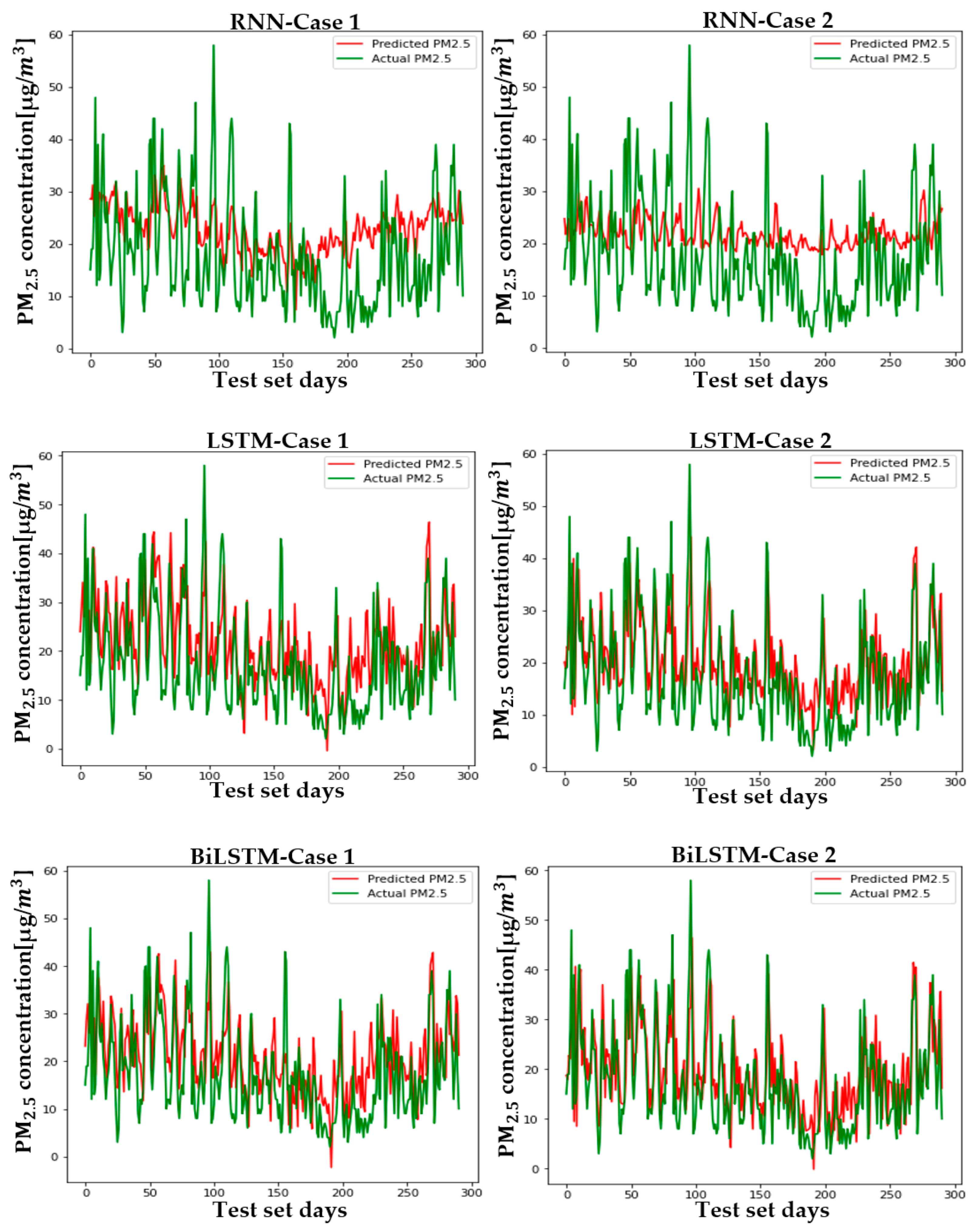
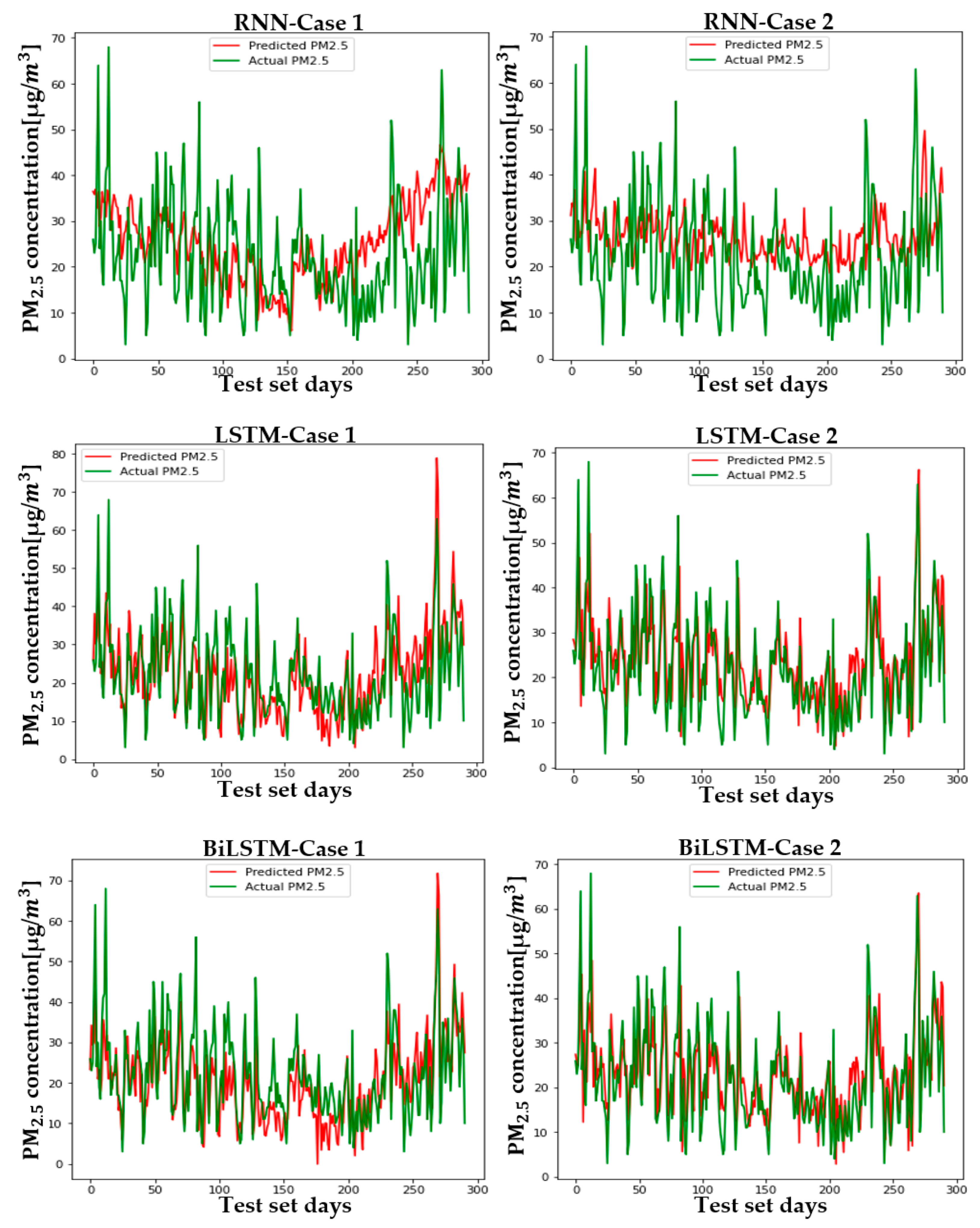
Figure 12 shows the predicted and actual values of PM2.5 for each case and model in Seoul. Figure A4, Figure A5, Figure A6, Figure A7, Figure A8, Figure A9 and Figure A10 show the PM2.5 concentration prediction of each city except for Seoul. Unlike LSTM and BiLSTM, the RNN appears to have outputted average values for all time periods and shows relatively low predictive power in both Case 1 and Case 2. The RNN without PCA seems to follow the trend more and to show relatively higher performance than the RNN with PCA. However, although there are differences between cities, LSTM and BiLSTM show that they follow the trend relatively well, regardless of whether PCA is applied or not. Furthermore, it can be seen that PCA application in all cities corrects the difference between the predicted and actual values that exists if PCA is not applied. It also appears to have produced more accurate results in predicting peak values.
Table 4 and Table 5 are numerical representations of these visual results. As noted above, it is understood that the reduction in dimension in all cities leads to a relatively low performance in the RNN, except for Daegu in terms of the MAE. This means that, for RNNs, reducing variables does not help model learning; rather, providing a high amount of information in a short period of time can lead to a better performance, depending on the feature of the model that relies on short-term information. Instead of an RNN, which lacks overall accuracy, the results that should be considered are those of LSTM and BiLSTM. Unlike the RNN, PCA application to LSTM and BiLSTM showed better results in RMSE and MAE evaluation, similar to the visual results. The order of cities with high performance is as follows: Busan > Daejeon > Gwangju > Daegu > Seoul > Ulsan > Wonju > Incheon, while the order of cities with high improvement in MAE and RMSE is as follows: Busan > Incheon > Gwangju > Seoul > Ulsan > Daegu > Daejeon > Wonju. LSTM showed high performance in Daejeon, Daegu, and Busan, while BiLSTM showed higher performance in the rest of the cities.
The difference in performance and performance improvements city by city makes it worthwhile to consider which characteristics of each city would cause regional differences in the performance of the same model, and which model would perform better depending on regional characteristics. To do so, it is expected that such studies require multidisciplinary considerations.
6. Conclusions
Performance degradation due to the curse of dimensionality can occur in deep learning and machine learning. We proposed a PCA-applied model to solve this problem, and through performance comparison with a non-PCA model, we showed that PCA applications produce better results in deep learning time series prediction. Such a performance improvement technique can be a way to increase the efficiency of the government system by providing better forecasts as a basis for issuing crisis alerts and establishing air pollution reduction policies in the future.
As the correlation analysis shows, the concentration of PM2.5 in China appears to have positive correlations with the concentration of PM2.5 in China, indicating that we have to consider China’s air pollution factors in predicting the concentration of PM2.5 in Korea. It suggests that there is a justification for the setup of real-time air pollution databases between the two countries from the ongoing joint research between Korea and China [38].
However, while PCA applications can improve model performance, the results show relatively weak predictions on predicting the minimum and maximum concentration PM2.5 for each city. It seems to be a problem due to a small number of observations (daily observations, not hourly observations). It is expected that future joint cross-border research will result in better performance by collecting much more observations. Some meteorological data in each Korean city showed a relatively weak correlation with concentration, so it seems necessary to find variables that have causality or strong correlation within areas other than deep learning. For example, if spatial factors (spatial homogeneity, autocorrelation, etc.) in Chinese cities and Korean cities are added to the model as input variables, it is expected that the model will produce better performance by learning time and spatial features of data.
This research will continue to maximize the prediction performance of deep learning models by collecting observations and optimizing models, while applying new algorithms and adding other variables that have causality with concentration of PM2.5 in terms of econometrics and spatial econometrics.
Author Contributions
Both authors have contributed to the ideas of the paper. S.W.C. analyzed the data, interpreted the results, and drafted the article. B.H.S.K. provided core advice, critically revised the article in terms of content and language, and approved this version for publication. Both authors have read and agreed to the published version of the manuscript.
Funding
This work was supported by the National Research Foundation of Korea (NRF) grant funded by the Ministry of Education (NRF-2020S1A5A2A01044582).
Institutional Review Board Statement
Not applicable.
Informed Consent Statement
Not applicable.
Data Availability Statement
Not applicable.
Acknowledgments
The open access fee was supported by the Research Institute for Agriculture and Life Sciences, Seoul National University.
Conflicts of Interest
The authors declare no conflict of interest.
Appendix A
Table A1 shows the acronym list of Table A2, Table A3, Table A4, Table A5, Table A6, Table A7, Table A8, Table A9, Table A10, Table A11, Table A12, Table A13, Table A14, Table A15, Table A16 and Table A17 and Figure A1, Figure A2 and Figure A3.

Table A1.
Acronym list.
| Acronym | Meaning |
|---|---|
| Min Temp | Minimum temperature (°C) |
| Max Temp | Maximum temperature (°C) |
| Mean Temp | Mean temperature (°C) |
| Daily prep | Daily precipitation (mm) |
| Max inst WS | Maximum instantaneous wind speed (m/s) |
| Max inst WSD | Maximum instantaneous wind speed directions (16 cardinal points) |
| Max WS | Maximum wind speed (m/s) |
| Max WSD | Maximum wind speed directions (16 cardinal points) |
| Mean WS | Mean wind speed (m/s) |
| WFS | Wind flow sum (100 m) |
| Max freq WD | Maximum frequent wind directions (16 cardinal points) |
| Mean DP | Mean dew point (°C) |
| Mean RH | Mean relative humidity (%) |
| Mean LAP | Mean local atmospheric pressure (hPa) |
| Max SP | Maximum sea-level pressure (hPa) |
| Min SP | Minimum sea-level pressure (hPa) |
| Mean SP | Mean sea-level pressure (hPa) |
| Min RH | Minimum relative humidity (%) |
| NPC | The number of principal components |
| CV | Cumulative variance |
Table A2, Table A3, Table A4, Table A5, Table A6, Table A7, Table A8 and Table A9 show the correlation coefficient of the meteorological and air quality factors between PM2.5 concentrations in each city.
Table A2.
The correlation coefficient of the meteorological and air quality factors between PM2.5 concentrations in Seoul.
Table A2.
The correlation coefficient of the meteorological and air quality factors between PM2.5 concentrations in Seoul.
| Air quality factors | O3 (ppm) | −0.021 | Meteorological factors | Min Temp | −0.175 | Max inst WS | −0.196 | Mean WS | −0.174 | Mean RH | 0.013 | Mean SP | 0.168 |
| CO (ppm) | 0.565 | Max Temp | −0.185 | Max inst WSD | 0.09 | WFS | −0.175 | Mean LAP | 0.166 | Min RH | −0.047 | ||
| NO2 (ppm) | 0.627 | Mean Temp | −0.156 | Max WS | −0.098 | Max freqWD | 0.041 | Max SP | 0.17 | ||||
| SO2 (ppm) | 0.417 | Daily prep | −0.143 | Max WSD | 0.118 | Mean DP | −0.141 | Min SP | 0.169 |
Table A3.
The correlation coefficient of the meteorological and air quality factors between PM2.5 concentrations in Gwangju.
Table A3.
The correlation coefficient of the meteorological and air quality factors between PM2.5 concentrations in Gwangju.
| Air quality factors | O3 (ppm) | 0.108 | Meteorological factors | Min Temp | −0.223 | Max inst WS | −0.226 | Mean WS | −0.28 | Mean RH | −0.164 | Mean SP | 0.192 |
| CO (ppm) | 0.532 | Max Temp | −0.122 | Max inst WSD | 0.108 | WFS | −0.281 | Mean LAP | 0.192 | Min RH | −0.235 | ||
| NO2 (ppm) | 0.562 | Mean Temp | −0.179 | Max WS | −0.214 | Max freq WD | 0.11 | Max SP | 0.186 | ||||
| SO2 (ppm) | 0.276 | Daily prep | −0.212 | Max WSD | 0.102 | Mean DP | −0.2 | Min SP | 0.196 |
Table A4.
The correlation coefficient of the meteorological and air quality factors between PM2.5 concentrations in Daegu.
Table A4.
The correlation coefficient of the meteorological and air quality factors between PM2.5 concentrations in Daegu.
| Air quality factors | O3 (ppm) | −0.113 | Meteorological factors | Min Temp | −0.291 | Max inst WS | −0.305 | Mean WS | −0.373 | Mean RH | −0.056 | Mean SP | 0.256 |
| CO (ppm) | 0.665 | Max Temp | −0.193 | Max inst WSD | 0.156 | WFS | −0.374 | Mean LAP | 0.252 | Min RH | −0.128 | ||
| NO2 (ppm) | 0.702 | Mean Temp | −0.244 | Max WS | −0.317 | Max freq WD | 0.053 | Max SP | 0.26 | ||||
| SO2 (ppm) | 0.437 | Daily prep | −0.157 | Max WSD | 0.14 | Mean DP | −0.214 | Min SP | 0.253 |
Table A5.
The correlation coefficient of the meteorological and air quality factors between PM2.5 concentrations in Daejeon.
Table A5.
The correlation coefficient of the meteorological and air quality factors between PM2.5 concentrations in Daejeon.
| Air quality factors | O3 (ppm) | −0.086 | Meteorological factors | Min Temp | −0.299 | Max ins tWS | −0.241 | Mean WS | −0.265 | Mean RH | −0.101 | Mean SP | 0.272 |
| CO (ppm) | 0.535 | Max Temp | −0.236 | Max inst WSD | 0.121 | WFS | −0.265 | Mean LAP | 0.271 | Min RH | −0.173 | ||
| NO2 (ppm) | 0.483 | Mean Temp | −0.272 | Max WS | −0.239 | Max freq WD | 0.211 | Max SP | 0.27 | ||||
| SO2 (ppm) | 0.41 | Daily prep | −0.18 | Max WSD | 0.1 | Mean DP | −0.271 | Min SP | 0.272 |
Table A6.
The correlation coefficient of the meteorological and air quality factors between PM2.5 concentrations in Busan.
Table A6.
The correlation coefficient of the meteorological and air quality factors between PM2.5 concentrations in Busan.
| Air quality factors | O3 (ppm) | 0.029 | Meteorological factors | Min Temp | −0.139 | Max inst WS | −0.231 | Mean WS | −0.162 | Mean RH | −0.126 | Mean SP | 0.104 |
| CO (ppm) | 0.32 | Max Temp | −0.095 | Max inst WSD | 0.196 | WFS | −0.162 | Mean LAP | 0.102 | Min RH | −0.187 | ||
| NO2 (ppm) | 0.554 | Mean Temp | −0.119 | Max WS | −0.07 | Max freqWD | 0.178 | Max SP | 0.086 | ||||
| SO2 (ppm) | 0.366 | Daily prep | −0.17 | Max WSD | 0.249 | Mean DP | −0.125 | Min SP | 0.124 |
Table A7.
The correlation coefficient of the meteorological and air quality factors between PM2.5 concentrations in Ulsan.
Table A7.
The correlation coefficient of the meteorological and air quality factors between PM2.5 concentrations in Ulsan.
| Air quality factors | O3 (ppm) | 0.095 | Meteorological factors | Min Temp | −0.084 | Max inst WS | −0.198 | Mean WS | −0.318 | Mean RH | −0.125 | Mean SP | 0.032 |
| CO (ppm) | 0.665 | Max Temp | 0.053 | Max inst WSD | 0.023 | WFS | −0.319 | Mean LAP | 0.064 | Min RH | −0.233 | ||
| NO2 (ppm) | 0.667 | Mean Temp | −0.015 | Max WS | −0.166 | Max freq WD | −0.055 | Max SP | 0.016 | ||||
| SO2 (ppm) | 0.525 | Daily prep | −0.167 | Max WSD | 0.014 | Mean DP | −0.055 | Min SP | 0.051 |
Table A8.
The correlation coefficient of the meteorological and air quality factors between PM2.5 concentrations in Wonju.
Table A8.
The correlation coefficient of the meteorological and air quality factors between PM2.5 concentrations in Wonju.
| Air quality factors | O3 (ppm) | −0.129 | Meteorological factors | Min Temp | −0.384 | Max inst WS | −0.187 | Mean WS | −0.257 | Mean RH | −0.018 | Mean SP | 0.309 |
| CO (ppm) | 0.686 | Max Temp | −0.339 | Max inst WSD | 0.171 | WFS | −0.259 | Mean LAP | 0.299 | Min RH | −0.077 | ||
| NO2 (ppm) | 0.675 | Mean Temp | −0.366 | Max WS | −0.187 | Max freq WD | 0.077 | Max SP | 0.318 | ||||
| SO2 (ppm) | 0.575 | Daily prep | −0.184 | Max WSD | 0.14 | Mean DP | −0.326 | Min SP | 0.302 |
Table A9.
The correlation coefficient of the meteorological and air quality factors between PM2.5 concentrations in Incheon.
Table A9.
The correlation coefficient of the meteorological and air quality factors between PM2.5 concentrations in Incheon.
| Air quality factors | O3 (ppm) | −0.102 | Meteorological Factors | Min Temp | −0.15 | Max inst WS | −0.288 | Mean WS | −0.308 | Mean RH | 0.214 | Mean SP | 0.149 |
| CO (ppm) | 0.621 | Max Temp | −0.122 | Max inst WSD | 0.045 | WFS | −0.309 | Mean LAP | 0.143 | Min RH | 0.091 | ||
| NO2 (ppm) | 0.667 | Mean Temp | −0.142 | Max WS | −0.254 | Max freq WD | 0.07 | Max SP | 0.155 | ||||
| SO2 (ppm) | 0.559 | Daily prep | −0.144 | Max WSD | 0.049 | Mean DP | −0.054 | Min SP | 0.151 |
Table A10, Table A11, Table A12, Table A13, Table A14, Table A15, Table A16 and Table A17 show the results of the PCA of each city.
Table A10.
The PCA result of Seoul.
| NPC | CV | NPC | CV | NPC | CV | NPC | CV | NPC | CV | NPC | CV | NPC | CV | NPC | CV |
|---|---|---|---|---|---|---|---|---|---|---|---|---|---|---|---|
| 1 | 82.06% | 11 | 97.88% | 21 | 98.99% | 31 | 99.49% | 41 | 99.77% | 51 | 99.92% | 61 | 99.99% | 71 | 100.00% |
| 2 | 93.11% | 12 | 98.04% | 22 | 99.06% | 32 | 99.52% | 42 | 99.79% | 52 | 99.93% | 62 | 100.00% | 72 | 100.00% |
| 3 | 94.58% | 13 | 98.19% | 23 | 99.12% | 33 | 99.56% | 43 | 99.81% | 53 | 99.94% | 63 | 100.00% | 73 | 100.00% |
| 4 | 95.71% | 14 | 98.33% | 24 | 99.18% | 34 | 99.59% | 44 | 99.82% | 54 | 99.95% | 64 | 100.00% | 74 | 100.00% |
| 5 | 96.31% | 15 | 98.45% | 25 | 99.23% | 35 | 99.62% | 45 | 99.84% | 55 | 99.96% | 65 | 100.00% | 75 | 100.00% |
| 6 | 96.69% | 16 | 98.56% | 26 | 99.28% | 36 | 99.65% | 46 | 99.85% | 56 | 99.97% | 66 | 100.00% | 76 | 100.00% |
| 7 | 97.01% | 17 | 98.66% | 27 | 99.33% | 37 | 99.68% | 47 | 99.87% | 57 | 99.98% | 67 | 100.00% | 77 | 100.00% |
| 8 | 97.28% | 18 | 98.76% | 28 | 99.37% | 38 | 99.70% | 48 | 99.88% | 58 | 99.98% | 68 | 100.00% | ||
| 9 | 97.50% | 19 | 98.85% | 29 | 99.41% | 39 | 99.72% | 49 | 99.90% | 59 | 99.99% | 69 | 100.00% | ||
| 10 | 97.70% | 20 | 98.92% | 30 | 99.45% | 40 | 99.75% | 50 | 99.91% | 60 | 99.99% | 70 | 100.00% |
Table A11.
The PCA result of Gwangju.
| NPC | CV | NPC | CV | NPC | CV | NPC | CV | NPC | CV | NPC | CV | NPC | CV | NPC | CV |
|---|---|---|---|---|---|---|---|---|---|---|---|---|---|---|---|
| 1 | 79.42% | 11 | 97.44% | 21 | 98.79% | 31 | 99.38% | 41 | 99.72% | 51 | 99.90% | 61 | 99.99% | 71 | 100.00% |
| 2 | 91.66% | 12 | 97.64% | 22 | 98.87% | 32 | 99.43% | 42 | 99.74% | 52 | 99.92% | 62 | 100.00% | 72 | 100.00% |
| 3 | 93.45% | 13 | 97.82% | 23 | 98.94% | 33 | 99.47% | 43 | 99.76% | 53 | 99.93% | 63 | 100.00% | 73 | 100.00% |
| 4 | 94.80% | 14 | 97.99% | 24 | 99.01% | 34 | 99.51% | 44 | 99.78% | 54 | 99.94% | 64 | 100.00% | 74 | 100.00% |
| 5 | 95.53% | 15 | 98.13% | 25 | 99.08% | 35 | 99.54% | 45 | 99.80% | 55 | 99.95% | 65 | 100.00% | 75 | 100.00% |
| 6 | 95.98% | 16 | 98.26% | 26 | 99.13% | 36 | 99.58% | 46 | 99.82% | 56 | 99.96% | 66 | 100.00% | 76 | 100.00% |
| 7 | 96.36% | 17 | 98.39% | 27 | 99.19% | 37 | 99.61% | 47 | 99.84% | 57 | 99.97% | 67 | 100.00% | 77 | 100.00% |
| 8 | 96.69% | 18 | 98.52% | 28 | 99.24% | 38 | 99.64% | 48 | 99.86% | 58 | 99.98% | 68 | 100.00% | ||
| 9 | 96.96% | 19 | 98.61% | 29 | 99.29% | 39 | 99.66% | 49 | 99.87% | 59 | 99.98% | 69 | 100.00% | ||
| 10 | 97.21% | 20 | 98.70% | 30 | 99.34% | 40 | 99.69% | 50 | 99.89% | 60 | 99.99% | 70 | 100.00% |
Table A12.
The PCA result of Daegu.
| NPC | CV | NPC | CV | NPC | CV | NPC | CV | NPC | CV | NPC | CV | NPC | CV | NPC | CV |
|---|---|---|---|---|---|---|---|---|---|---|---|---|---|---|---|
| 1 | 89.40% | 11 | 98.69% | 21 | 99.38% | 31 | 99.69% | 41 | 99.86% | 51 | 99.95% | 61 | 100.00% | 71 | 100.00% |
| 2 | 95.70% | 12 | 98.79% | 22 | 99.42% | 32 | 99.71% | 42 | 99.87% | 52 | 99.96% | 62 | 100.00% | 72 | 100.00% |
| 3 | 96.62% | 13 | 98.88% | 23 | 99.46% | 33 | 99.73% | 43 | 99.88% | 53 | 99.97% | 63 | 100.00% | 73 | 100.00% |
| 4 | 97.33% | 14 | 98.96% | 24 | 99.49% | 34 | 99.75% | 44 | 99.89% | 54 | 99.97% | 64 | 100.00% | 74 | 100.00% |
| 5 | 97.70% | 15 | 99.04% | 25 | 99.53% | 35 | 99.77% | 45 | 99.90% | 55 | 99.98% | 65 | 100.00% | 75 | 100.00% |
| 6 | 97.93% | 16 | 99.11% | 26 | 99.56% | 36 | 99.79% | 46 | 99.91% | 56 | 99.98% | 66 | 100.00% | 76 | 100.00% |
| 7 | 98.13% | 17 | 99.17% | 27 | 99.59% | 37 | 99.80% | 47 | 99.92% | 57 | 99.99% | 67 | 100.00% | 77 | 100.00% |
| 8 | 98.30% | 18 | 99.23% | 28 | 99.61% | 38 | 99.82% | 48 | 99.93% | 58 | 99.99% | 68 | 100.00% | ||
| 9 | 98.44% | 19 | 99.28% | 29 | 99.64% | 39 | 99.83% | 49 | 99.94% | 59 | 99.99% | 69 | 100.00% | ||
| 10 | 98.57% | 20 | 99.33% | 30 | 99.66% | 40 | 99.85% | 50 | 99.95% | 60 | 100.00% | 70 | 100.00% |
Table A13.
The PCA result of Daejeon.
| NPC | CV | NPC | CV | NPC | CV | NPC | CV | NPC | CV | NPC | CV | NPC | CV | NPC | CV |
|---|---|---|---|---|---|---|---|---|---|---|---|---|---|---|---|
| 1 | 78.91% | 11 | 97.36% | 21 | 98.74% | 31 | 99.36% | 41 | 99.71% | 51 | 99.91% | 61 | 99.99% | 71 | 100.00% |
| 2 | 91.31% | 12 | 97.56% | 22 | 98.82% | 32 | 99.41% | 42 | 99.74% | 52 | 99.92% | 62 | 100.00% | 72 | 100.00% |
| 3 | 93.19% | 13 | 97.75% | 23 | 98.90% | 33 | 99.45% | 43 | 99.76% | 53 | 99.93% | 63 | 100.00% | 73 | 100.00% |
| 4 | 94.62% | 14 | 97.92% | 24 | 98.97% | 34 | 99.49% | 44 | 99.78% | 54 | 99.95% | 64 | 100.00% | 74 | 100.00% |
| 5 | 95.39% | 15 | 98.06% | 25 | 99.04% | 35 | 99.53% | 45 | 99.81% | 55 | 99.96% | 65 | 100.00% | 75 | 100.00% |
| 6 | 95.86% | 16 | 98.20% | 26 | 99.10% | 36 | 99.57% | 46 | 99.83% | 56 | 99.97% | 66 | 100.00% | 76 | 100.00% |
| 7 | 96.26% | 17 | 98.33% | 27 | 99.16% | 37 | 99.60% | 47 | 99.84% | 57 | 99.97% | 67 | 100.00% | 77 | 100.00% |
| 8 | 96.60% | 18 | 98.45% | 28 | 99.21% | 38 | 99.63% | 48 | 99.86% | 58 | 99.98% | 68 | 100.00% | ||
| 9 | 96.88% | 19 | 98.55% | 29 | 99.26% | 39 | 99.66% | 49 | 99.88% | 59 | 99.99% | 69 | 100.00% | ||
| 10 | 97.13% | 20 | 98.65% | 30 | 99.31% | 40 | 99.69% | 50 | 99.89% | 60 | 99.99% | 70 | 100.00% |
Table A14.
The PCA result of Busan.
| NPC | CV | NPC | CV | NPC | CV | NPC | CV | NPC | CV | NPC | CV | NPC | CV | NPC | CV |
|---|---|---|---|---|---|---|---|---|---|---|---|---|---|---|---|
| 1 | 90.96% | 11 | 98.92% | 21 | 99.49% | 31 | 99.74% | 41 | 99.88% | 51 | 99.96% | 61 | 100.00% | 71 | 100.00% |
| 2 | 96.47% | 12 | 99.00% | 22 | 99.52% | 32 | 99.75% | 42 | 99.89% | 52 | 99.97% | 62 | 100.00% | 72 | 100.00% |
| 3 | 97.22% | 13 | 99.08% | 23 | 99.55% | 33 | 99.77% | 43 | 99.90% | 53 | 99.97% | 63 | 100.00% | 73 | 100.00% |
| 4 | 97.79% | 14 | 99.15% | 24 | 99.58% | 34 | 99.79% | 44 | 99.91% | 54 | 99.98% | 64 | 100.00% | 74 | 100.00% |
| 5 | 98.10% | 15 | 99.21% | 25 | 99.61% | 35 | 99.80% | 45 | 99.92% | 55 | 99.98% | 65 | 100.00% | 75 | 100.00% |
| 6 | 98.30% | 16 | 99.27% | 26 | 99.63% | 36 | 99.82% | 46 | 99.93% | 56 | 99.98% | 66 | 100.00% | 76 | 100.00% |
| 7 | 98.47% | 17 | 99.32% | 27 | 99.65% | 37 | 99.83% | 47 | 99.93% | 57 | 99.99% | 67 | 100.00% | 77 | 100.00% |
| 8 | 98.60% | 18 | 99.37% | 28 | 99.68% | 38 | 99.85% | 48 | 99.94% | 58 | 99.99% | 68 | 100.00% | ||
| 9 | 98.72% | 19 | 99.41% | 29 | 99.70% | 39 | 99.86% | 49 | 99.95% | 59 | 99.99% | 69 | 100.00% | ||
| 10 | 98.83% | 20 | 99.45% | 30 | 99.72% | 40 | 99.87% | 50 | 99.95% | 60 | 100.00% | 70 | 100.00% |
Table A15.
The PCA result of Ulsan.
| NPC | CV | NPC | CV | NPC | CV | NPC | CV | NPC | CV | NPC | CV | NPC | CV | NPC | CV |
|---|---|---|---|---|---|---|---|---|---|---|---|---|---|---|---|
| 1 | 83.59% | 11 | 98.04% | 21 | 99.07% | 31 | 99.52% | 41 | 99.78% | 51 | 99.92% | 61 | 99.99% | 71 | 100.00% |
| 2 | 93.60% | 12 | 98.19% | 22 | 99.13% | 32 | 99.55% | 42 | 99.80% | 52 | 99.93% | 62 | 100.00% | 72 | 100.00% |
| 3 | 94.97% | 13 | 98.32% | 23 | 99.18% | 33 | 99.58% | 43 | 99.82% | 53 | 99.94% | 63 | 100.00% | 73 | 100.00% |
| 4 | 96.00% | 14 | 98.45% | 24 | 99.24% | 34 | 99.61% | 44 | 99.83% | 54 | 99.95% | 64 | 100.00% | 74 | 100.00% |
| 5 | 96.55% | 15 | 98.56% | 25 | 99.28% | 35 | 99.64% | 45 | 99.85% | 55 | 99.96% | 65 | 100.00% | 75 | 100.00% |
| 6 | 96.90% | 16 | 98.66% | 26 | 99.33% | 36 | 99.67% | 46 | 99.86% | 56 | 99.97% | 66 | 100.00% | 76 | 100.00% |
| 7 | 97.21% | 17 | 98.76% | 27 | 99.37% | 37 | 99.69% | 47 | 99.88% | 57 | 99.97% | 67 | 100.00% | 77 | 100.00% |
| 8 | 97.46% | 18 | 98.86% | 28 | 99.41% | 38 | 99.71% | 48 | 99.89% | 58 | 99.98% | 68 | 100.00% | ||
| 9 | 97.68% | 19 | 98.93% | 29 | 99.45% | 39 | 99.74% | 49 | 99.90% | 59 | 99.99% | 69 | 100.00% | ||
| 10 | 97.87% | 20 | 99.00% | 30 | 99.48% | 40 | 99.76% | 50 | 99.91% | 60 | 99.99% | 70 | 100.00% |
Table A16.
The PCA result of Wonju.
| NPC | CV | NPC | CV | NPC | CV | NPC | CV | NPC | CV | NPC | CV | NPC | CV | NPC | CV |
|---|---|---|---|---|---|---|---|---|---|---|---|---|---|---|---|
| 1 | 71.67% | 11 | 96.38% | 21 | 98.28% | 31 | 99.13% | 41 | 99.61% | 51 | 99.87% | 61 | 99.99% | 71 | 100.00% |
| 2 | 88.12% | 12 | 96.65% | 22 | 98.39% | 32 | 99.19% | 42 | 99.64% | 52 | 99.89% | 62 | 100.00% | 72 | 100.00% |
| 3 | 90.65% | 13 | 96.91% | 23 | 98.50% | 33 | 99.25% | 43 | 99.68% | 53 | 99.91% | 63 | 100.00% | 73 | 100.00% |
| 4 | 92.60% | 14 | 97.14% | 24 | 98.60% | 34 | 99.31% | 44 | 99.71% | 54 | 99.92% | 64 | 100.00% | 74 | 100.00% |
| 5 | 93.66% | 15 | 97.34% | 25 | 98.69% | 35 | 99.36% | 45 | 99.73% | 55 | 99.94% | 65 | 100.00% | 75 | 100.00% |
| 6 | 94.32% | 16 | 97.53% | 26 | 98.77% | 36 | 99.41% | 46 | 99.76% | 56 | 99.95% | 66 | 100.00% | 76 | 100.00% |
| 7 | 94.86% | 17 | 97.71% | 27 | 98.85% | 37 | 99.45% | 47 | 99.78% | 57 | 99.96% | 67 | 100.00% | 77 | 100.00% |
| 8 | 95.33% | 18 | 97.88% | 28 | 98.93% | 38 | 99.50% | 48 | 99.81% | 58 | 99.97% | 68 | 100.00% | ||
| 9 | 95.71% | 19 | 98.02% | 29 | 99.00% | 39 | 99.54% | 49 | 99.83% | 59 | 99.98% | 69 | 100.00% | ||
| 10 | 96.05% | 20 | 98.15% | 30 | 99.06% | 40 | 99.57% | 50 | 99.85% | 60 | 99.98% | 70 | 100.00% |
Table A17.
The PCA result of Incheon.
| NPC | CV | NPC | CV | NPC | CV | NPC | CV | NPC | CV | NPC | CV | NPC | CV | NPC | CV |
|---|---|---|---|---|---|---|---|---|---|---|---|---|---|---|---|
| 1 | 91.12% | 11 | 98.93% | 21 | 99.49% | 31 | 99.74% | 41 | 99.88% | 51 | 99.96% | 61 | 100.00% | 71 | 100.00% |
| 2 | 96.52% | 12 | 99.01% | 22 | 99.52% | 32 | 99.75% | 42 | 99.89% | 52 | 99.96% | 62 | 100.00% | 72 | 100.00% |
| 3 | 97.25% | 13 | 99.08% | 23 | 99.55% | 33 | 99.77% | 43 | 99.90% | 53 | 99.97% | 63 | 100.00% | 73 | 100.00% |
| 4 | 97.83% | 14 | 99.15% | 24 | 99.58% | 34 | 99.79% | 44 | 99.91% | 54 | 99.97% | 64 | 100.00% | 74 | 100.00% |
| 5 | 98.12% | 15 | 99.21% | 25 | 99.61% | 35 | 99.80% | 45 | 99.92% | 55 | 99.98% | 65 | 100.00% | 75 | 100.00% |
| 6 | 98.31% | 16 | 99.27% | 26 | 99.63% | 36 | 99.82% | 46 | 99.92% | 56 | 99.98% | 66 | 100.00% | 76 | 100.00% |
| 7 | 98.47% | 17 | 99.32% | 27 | 99.65% | 37 | 99.83% | 47 | 99.93% | 57 | 99.99% | 67 | 100.00% | 77 | 100.00% |
| 8 | 98.61% | 18 | 99.37% | 28 | 99.68% | 38 | 99.84% | 48 | 99.94% | 58 | 99.99% | 68 | 100.00% | ||
| 9 | 98.72% | 19 | 99.42% | 29 | 99.70% | 39 | 99.85% | 49 | 99.95% | 59 | 99.99% | 69 | 100.00% | ||
| 10 | 98.83% | 20 | 99.45% | 30 | 99.72% | 40 | 99.87% | 50 | 99.95% | 60 | 99.99% | 70 | 100.00% |
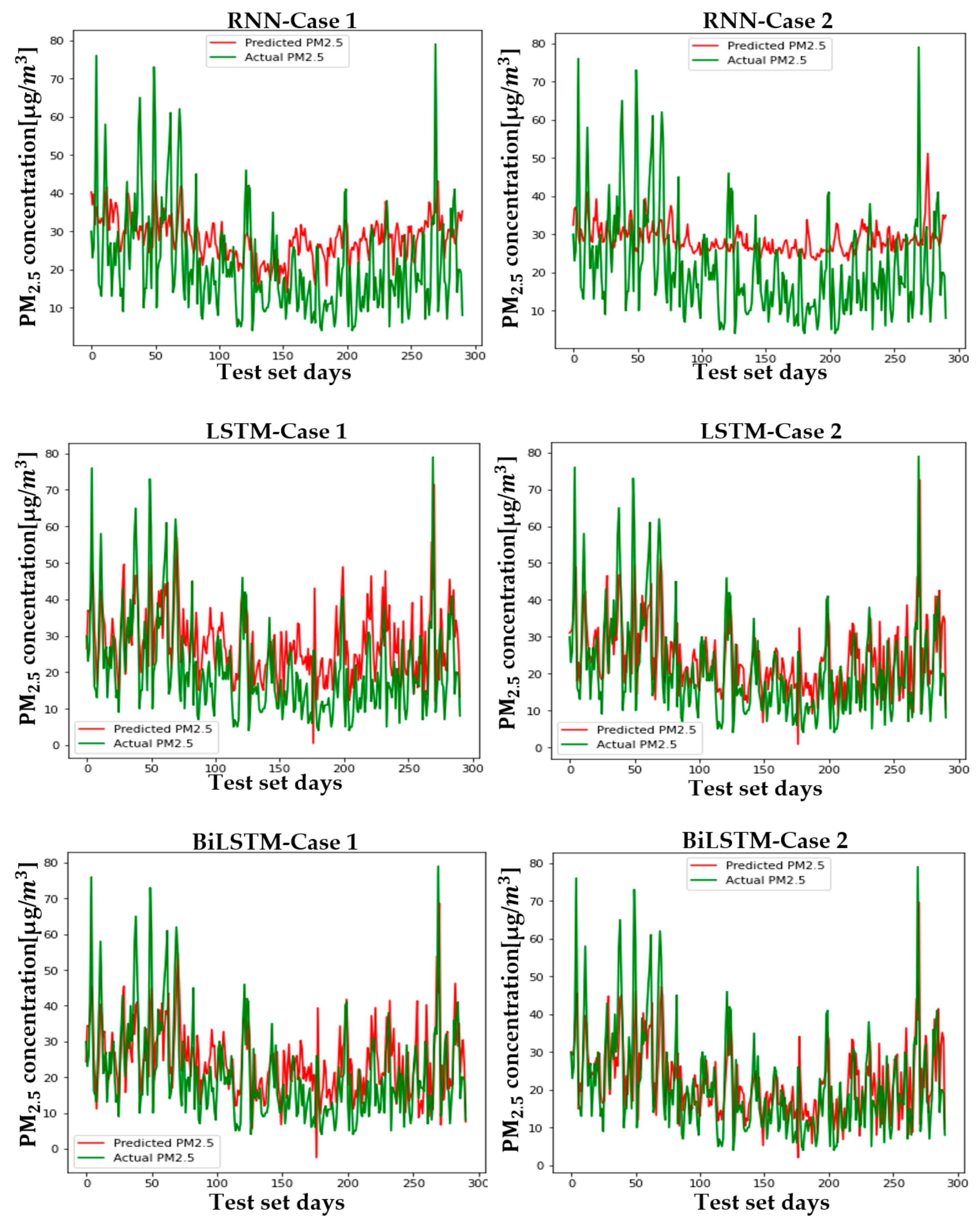
Figure A1, Figure A2 and Figure A3 show the meteorological data of Seoul and Figure A4, Figure A5, Figure A6, Figure A7, Figure A8, Figure A9 and Figure A10 show the PM2.5 concentration prediction of each city.
Figure A1.
The meteorological data of Seoul (atmospheric, sea−level pressure).

Figure A2.
The meteorological data of Seoul (wind).

Figure A3.
The meteorological data of Seoul (temperature, relative humidity, precipitation).

Figure A4.
The PM2.5 prediction in Gwangju by two cases.

Figure A5.
The PM2.5 prediction in Daegu by two cases.

Figure A6.
The PM2.5 prediction in Daejeon by two cases.

Figure A7.
The PM2.5 prediction in Busan by two cases.

Figure A8.
The PM2.5 prediction in Ulsan by two cases.

Figure A9.
The PM2.5 prediction in Wonju by two cases.

Figure A10.
The PM2.5 prediction in Incheon by two cases.

References
- Gong, S. A Study on the Health Impact and Management Policy of PM2.5 in Korea 1.; Korea Environment Institute: Sejong, Korea, 2012; pp. 1–209. (In Korean) [Google Scholar]
- WHO Health Organization. Ambient (Outdoor) Air Pollution. Available online: https://www.who.int/news-room/fact-sheets/detail/ambient-(outdoor)-air-quality-and-health (accessed on 8 December 2019).
- French National Health Agency, InVS, European Environment Agency. Available online: https://news.yahoo.com/micro-pollution-ravaging-china-south-asia-study-031634307.html (accessed on 3 March 2020).
- OECD. Available online: https://data.oecd.org/air/air-pollution-exposure.htm (accessed on 11 December 2019).
- Han, C.; Kim, S.; Lim, Y.-H.; Bae, H.-J.; Hong, Y.-C. Spatial and Temporal Trends of Number of Deaths Attributable to Ambient PM2.5in the Korea. J. Korean Med Sci. 2018, 33, e193. [Google Scholar] [CrossRef]
- Hwang, I.C.; Kim, C.H.; Son, W.I. Benefits of Management Policy of Seoul on Airborne Particulate Matter; The Seoul Institute Policy Research: Seoul, Korea, 2018; pp. 1–113. (In Korean) [Google Scholar]
- Statistics Korea Office Press Release. “Results of Cause of Death Statistics in 2019”, Statistics Korea. Available online: http://kostat.go.kr/portal/korea/kor_nw/1/6/2/index.board?bmode=read&bSeq=&aSeq=385219&pageNo=1&rowNum=10&navCount=10&currPg=&searchInfo=&sTarget=title&sTxt= (accessed on 22 September 2020). (In Korean).
- Joint Association of Related Korean Ministries of Korea. Comprehensive Plan for Fine Dust Management (2020–2024); Joint Association of Related Korean Ministries of Korea: Seoul, Korea, 2019. (In Korean) [Google Scholar]
- Xayasouk, T.; Lee, H.; Lee, G. Air Pollution Prediction Using Long Short-Term Memory (LSTM) and Deep Autoencoder (DAE) Models. Sustainability 2020, 12, 2570. [Google Scholar] [CrossRef] [Green Version]
- Mengara, A.M.; Kim, Y.; Yoo, Y.; Ahn, J. Distributed Deep Features Extraction Model for Air Quality Forecasting. Sustainability 2020, 12, 8014. [Google Scholar] [CrossRef]
- Park, S.; Shin, H. Analysis of the Factors Influencing PM2.5 in Korea: Focusing on Seasonal Factors. J. Environ. Policy Adm. 2017, 25, 227–248. (In Korean) [Google Scholar] [CrossRef]
- Wang, C.; Tu, Y.; Yu, Z.; Lu, R. PM2.5 and Cardiovascular Diseases in the Elderly: An Overview. Int. J. Environ. Res. Public Heal. 2015, 12, 8187–8197. [Google Scholar] [CrossRef] [Green Version]
- César, A.C.G.; Nascimento, L.F.C.; Mantovani, K.C.C.; Vieira, L.C.P. Fine particulate matter estimated by mathematical model and hospitalizations for pneumonia and asthma in children. Rev. Paul. Pediatr. 2016, 34, 18–23. [Google Scholar] [CrossRef] [PubMed]
- Kim, K.-N.; Kim, S.; Lim, Y.-H.; Song, I.G.; Hong, Y.-C. Effects of short-term fine particulate matter exposure on acute respiratory infection in children. Int. J. Hyg. Environ. Health 2020, 229, 113571. [Google Scholar] [CrossRef]
- Vinikoor-Imler, L.C.; Davis, J.A.; Luben, T.J. An Ecologic Analysis of County-Level PM2.5 Concentrations and Lung Cancer Incidence and Mortality. Int. J. Environ. Res. Public Health 2011, 8, 1865–1871. [Google Scholar] [CrossRef]
- Choe, J.-I.; Lee, Y.S. A Study on the Impact of PM2.5 Emissions on Respiratory Diseases. J. Environ. Policy Adm. 2015, 23, 155. (In Korean) [Google Scholar] [CrossRef]
- Ross, Z.; Jerrett, M.; Ito, K.; Tempalski, B.; Thurston, G. A land use regression for predicting fine particulate matter concentrations in the New York City region. Atmos. Environ. 2007, 41, 2255–2269. [Google Scholar] [CrossRef]
- Beelen, R.; Hoek, G.; Pebesma, E.; Vienneau, D.; de Hoogh, K.; Briggs, D.J. Mapping of background air pollution at a fine spatial scale across the European Union. Sci. Total. Environ. 2009, 407, 1852–1867. [Google Scholar] [CrossRef] [PubMed]
- Singh, V.; Carnevale, C.; Finzi, G.; Pisoni, E.; Volta, M. A cokriging based approach to reconstruct air pollution maps, processing measurement station concentrations and deterministic model simulations. Environ. Model. Softw. 2011, 26, 778–786. [Google Scholar] [CrossRef]
- Zhao, J.; Deng, F.; Cai, Y.; Chen, J. Long short-term memory—Fully connected (LSTM-FC) neural network for PM2.5 concentration prediction. Chemosphere 2019, 220, 486–492. [Google Scholar] [CrossRef] [PubMed]
- Karimian, H.; Li, Q.; Wu, C.; Qi, Y.; Mo, Y.; Chen, G.; Zhang, X.; Sachdeva, S. Evaluation of Different Machine Learning Approaches to Forecasting PM2.5 Mass Concentrations. Aerosol Air Qual. Res. 2019, 19, 1400–1410. [Google Scholar] [CrossRef] [Green Version]
- Qadeer, K.; Rehman, W.U.; Sheri, A.M.; Park, I.; Kim, H.K.; Jeon, M. A Long Short-Term Memory (LSTM) Network for Hourly Estimation of PM2.5 Concentration in Two Cities of South Korea. Appl. Sci. 2020, 10, 3984. [Google Scholar] [CrossRef]
- Air Korea. Available online: http://www.airkorea.or.kr/web (accessed on 30 January 2020). (In Korean).
- Korea Meteorological Agency. Available online: https://data.kma.go.kr/cmmn/main.do (accessed on 15 February 2019). (In Korean).
- Nullschool. Available online: https://earth.nullschool.net/ko/ (accessed on 30 January 2020).
- Bao, R.; Zhang, A. Does lockdown reduce air pollution? Evidence from 44 cities in northern China. Sci. Total Environ. 2020, 731, 139052. [Google Scholar] [CrossRef] [PubMed]
- Moritz, S.; Bartz-Beielstein, T. imputeTS: Time Series Missing Value Imputation in R. R J. 2017, 9, 207–218. [Google Scholar] [CrossRef] [Green Version]
- Hunter, J.S. The Exponentially Weighted Moving Average. J. Qual. Technol. 1986, 18, 203–210. [Google Scholar] [CrossRef]
- China National Environmental Monitoring Centre. Available online: http://www.cnemc.cn/sssj/ (accessed on 1 March 2020). (In Chinese).
- Hsieh, T.-J.; Hsiao, H.-F.; Yeh, W.-C. Forecasting stock markets using wavelet transforms and recurrent neural networks: An integrated system based on artificial bee colony algorithm. Appl. Soft Comput. 2011, 11, 2510–2525. [Google Scholar] [CrossRef]
- Franklin, J.A. Recurrent Neural Networks for Music Computation. INFORMS J. Comput. 2006, 18, 321–338. [Google Scholar] [CrossRef] [Green Version]
- Goldberg, Y. Neural Network Methods for Natural Language Processing. Synth. Lect. Hum. Lang. Technol. 2017, 10, 1–309. [Google Scholar] [CrossRef]
- Chen, G. A gentle tutorial of recurrent neural network with error backpropagation. arXiv 2016, arXiv:1610.02583. [Google Scholar]
- Hochreiter, S.; Schmidhuber, J. Long Short-Term Memory. Neural Comput. 1997, 9, 1735–1780. [Google Scholar] [CrossRef] [PubMed]
- Schuster, M.; Paliwal, K. Bidirectional recurrent neural networks. IEEE Trans. Signal Process. 1997, 45, 2673–2681. [Google Scholar] [CrossRef] [Green Version]
- Gonzalez, J.; Yu, W. Non-linear system modeling using LSTM neural networks. IFAC-PapersOnLine 2018, 51, 485–489. [Google Scholar] [CrossRef]
- Kingma, D.P.; Ba, J. Adam: A method for stochastic optimization. In Proceedings of the International Conference Learn, Represent (ICLR), San Diego, CA, USA, 5–8 May 2015. [Google Scholar]
- Ministry of Environment. Ministry of Environment Press Release “Korea-China Joint Research Group to Reduce Fine Dust”. Available online: http://me.go.kr/home/web/board/read.do?boardMasterId=1&boardId=1201300&menuId=286 (accessed on 22 January 2020). (In Korean)
Figure 1.
Effects of fine particulate matter (PM2.5) on the body. Source: French National Health Agency, InVS (Institut de veille sanitaire), European Environment Agency, and AFP.
Figure 1.
Effects of fine particulate matter (PM2.5) on the body. Source: French National Health Agency, InVS (Institut de veille sanitaire), European Environment Agency, and AFP.

Figure 2.
Spatial range of the research.

Figure 3.
The wind direction frequency of Korea’s selected cities in 2019.

Figure 4.
PM2.5 distribution maps (before and after the COVID-19 outbreak: 2019 vs. 2020).

Figure 5.
Visualization of China’s and Seoul’s air quality data set.

Figure 6.
Correlation between the highest eight factors and PM2.5 concentrations in Seoul, Korea.

Figure 7.
Origin–destination map of PM2.5 correlations between Chinese cities and Korean cities.

Figure 8.
Internal structure of the recurrent neural network (RNN).

Figure 9.
Internal structure of long short-term memory (LSTM).

Figure 10.
Internal structure of bidirectional long short-term memory (BiLSTM) and an example.

Figure 11.
Workflow of the PCA application deep learning model for predicting PM2.5.

Figure 12.
The PM2.5 prediction in Seoul by two cases.

Table 1.
Crisis stage standard.
| Crisis Stages | Criteria | Main Contents |
|---|---|---|
| Stage 1 | 150 μg/m3 for 2 h or longer + 75 μg/m3 for the following day | Strengthening the current system |
| Stage 2 | 200 μg/m3 for 2 h or longer + 150 μg/m3 for the following day | Strengthening public sector measures |
| Stage 3 | 400 μg/m3 for 2 h or longer + 200 μg/m3 for the following day | Strengthening private sector measures/disaster response |
Table 2.
Correlation range from Chinese cities to Korean cities.
| Cities | Minimum | Maximum | Cities | Minimum | Maximum |
|---|---|---|---|---|---|
| Seoul | 0.1993 | 0.4994 | Busan | 0.1320 | 0.5084 |
| Gwangju | 0.1446 | 0.4035 | Ulsan | 0.1419 | 0.5394 |
| Daegu | 0.1813 | 0.5087 | Wonju | 0.1824 | 0.5550 |
| Daejeon | 0.1839 | 0.5087 | Incheon | 0.2556 | 0.5415 |
Table 3.
The ratio of variance explained by five principal components in each city.
| Cities | Cumulative Variance | Cities | Cumulative Variance |
|---|---|---|---|
| Seoul | 0.9631(=96.31%) | Busan | 0.98102(=98.102%) |
| Gwangju | 0.9553(=95.53%) | Ulsan | 0.9655(=96.55%) |
| Daegu | 0.9770(=97.70%) | Wonju | 0.9366(=93.66%) |
| Daejeon | 0.9539(=95.39%) | Incheon | 0.98123(=98.123%) |
Table 4.
Evaluation results from PM2.5 prediction in each Korean city (Case 1).
| City | Model | RMSE | MAE | City | Model | RMSE | MAE |
|---|---|---|---|---|---|---|---|
| Seoul | RNN | 9.730 | 7.328 | Gwangju | RNN | 9.002 | 7.472 |
| LSTM | 8.020 | 6.374 | LSTM | 7.7415 | 5.797 | ||
| BiLSTM | 8.101 | 6.168 | BiLSTM | 8.300 | 6.590 | ||
| Daegu | RNN | 10.171 | 8.110 | Busan | RNN | 8.410 | 7.224 |
| LSTM | 7.654 | 6.223 | LSTM | 7.770 | 6.504 | ||
| BiLSTM | 7.707 | 6.193 | BiLSTM | 7.897 | 6.578 | ||
| Daejeon | RNN | 9.361 | 7.497 | Ulsan | RNN | 10.558 | 8.988 |
| LSTM | 7.042 | 5.753 | LSTM | 8.660 | 6.959 | ||
| BiLSTM | 7.231 | 5.927 | BiLSTM | 8.383 | 6.772 | ||
| Wonju | RNN | 11.603 | 9.208 | Incheon | RNN | 13.686 | 11.408 |
| LSTM | 8.718 | 6.520 | LSTM | 11.900 | 9.828 | ||
| BiLSTM | 8.459 | 6.251 | BiLSTM | 10.393 | 8.285 |
Table 5.
Evaluation results from PM2.5 prediction in each Korean city (Case 2).
| City | Model | RMSE | MAE | City | Model | RMSE | MAE |
|---|---|---|---|---|---|---|---|
| Seoul | RNN | 11.680 (20%↑) | 9.310 (27%↑) | Gwangju | RNN | 9.492 (5.4%↑) | 7.746 (3.7%↑) |
| LSTM | 7.667 (4.6%↓) | 5.455 (16.8%↓) | LSTM | 7.148 (8.3%↓) | 5.541 (4.6%↓) | ||
| BiLSTM | 7.567 (7.1%↓) | 5.368 (14.9%↓) | BiLSTM | 7.110 (16.7%↓) | 5.455 (20.8%↓) | ||
| Daegu | RNN | 10.208 (0.4%↑) | 7.824 (3.5%↓) | Busan | RNN | 9.924 (18%↑) | 8.316 (15.1%↑) |
| LSTM | 7.491 (2.2%↓) | 5.664 (9.9%↓) | LSTM | 6.668 (16.5%↓) | 4.881 (33.3%↓) | ||
| BiLSTM | 7.552 (2.1%↓) | 5.703 (8.6%↓) | BiLSTM | 6.779 (16.5%↓) | 4.999 (31.6%↓) | ||
| Daejeon | RNN | 9.602 (2.6%↑) | 7.824 (4.4%↑) | Ulsan | RNN | 11.160 (5.7%↑) | 9.389 (4.5%↑) |
| LSTM | 6.967 (1.1%↓) | 5.374 (7.1%↓) | LSTM | 8.021 (8%↓) | 6.251 (11.3%↓) | ||
| BiLSTM | 7.098 (1.9%↓) | 5.537 (7%↓) | BiLSTM | 7.871 (6.5%↓) | 5.993 (13%↓) | ||
| Wonju | RNN | 12.132 (4.6%↑) | 9.758 (6%↑) | Incheon | RNN | 14.744 (7.7%↑) | 12.427 (8.9%↑) |
| LSTM | 8.424 (3.5%↓) | 6.251 (4.3%↓) | LSTM | 10.205 (16.6%↓) | 8.000 (22.9%↓) | ||
| BiLSTM | 8.345 (1.4%↓) | 6.137 (1.9%↓) | BiLSTM | 9.709 (7%↓) | 7.354 (12.7%↓) |
Publisher’s Note: MDPI stays neutral with regard to jurisdictional claims in published maps and institutional affiliations. |
© 2021 by the authors. Licensee MDPI, Basel, Switzerland. This article is an open access article distributed under the terms and conditions of the Creative Commons Attribution (CC BY) license (http://creativecommons.org/licenses/by/4.0/).
Share and Cite
MDPI and ACS Style
Choi, S.W.; Kim, B.H.S. Applying PCA to Deep Learning Forecasting Models for Predicting PM2.5. Sustainability 2021, 13, 3726. https://0-doi-org.brum.beds.ac.uk/10.3390/su13073726
AMA Style
Choi SW, Kim BHS. Applying PCA to Deep Learning Forecasting Models for Predicting PM2.5. Sustainability. 2021; 13(7):3726. https://0-doi-org.brum.beds.ac.uk/10.3390/su13073726
Chicago/Turabian StyleChoi, Sang Won, and Brian H. S. Kim. 2021. "Applying PCA to Deep Learning Forecasting Models for Predicting PM2.5" Sustainability 13, no. 7: 3726. https://0-doi-org.brum.beds.ac.uk/10.3390/su13073726
Note that from the first issue of 2016, this journal uses article numbers instead of page numbers. See further details here.