1. Introduction
A project can be defined as a “‘unique, temporary, multidisciplinary and organized endeavor to realize agreed deliverables within pre-defined requirements and constraints” [
1]. Industrial construction projects, which fall under this definition, have their own peculiarities, one of the most relevant being their complexity due to the multiple variables, components, and activities that must be managed, coordinated, and controlled in each phase. They are part of various construction markets, but different from civil construction, infrastructure, or residential buildings, being their purpose to deliver a functioning facility or asset to End-Users. This type of projects encompasses a wide variety of fields of application and sectors, including but not limited to power generation, nuclear plants, industrial plants, renewables, power transmission and distribution, water treatment, Oil and Gas fields development and processing plants or treatment units [
2,
3,
4,
5,
6].
In this study, there is considered hypothetical planning data from a set of power generation projects (PXE) and one non-power generation project (INE), all of them carried out under the EPC (Engineering, Procurement, and Construction) form of contracting arrangement. The EPC contractor is responsible for all the activities during the execution phase, including the design engineering, the procurement, and supply of the necessary equipment and materials, the construction, along with the installation, commissioning and start-up of the facility or asset in order to complete the scope of works necessary for the handover of the project to the Client.
The prominence of EPC projects is clear from the figures for the international procurement market, which shows that EPC contracts were worth an estimated USD 7.60 trillion at the end of 2019 [
7], although this project model is coming under increasing pressure due to low productivity, tight profit margins or lack of digitization [
8]. Improving the efficiency of projects to minimize problems between the parties involved, optimize execution, and control operating and maintenance costs become an indispensable task given the multitude of simultaneous activities that are extremely complicated to manage [
9,
10,
11], especially since they are heavily conditioned by cost margins and deadlines.
Numerous methodologies and tools have been developed and implemented to manage projects, despite which the number of failed projects remains high [
1]. Industrial construction projects are no exception, where a clear example of this can be found in EPC contracts, which very often experience high-cost overruns and significant delays [
12,
13,
14,
15]. Over the last years, diverse studies have tried to identify the variety of reasons for delays in projects and proposed methods to mitigate them by analyzing different aspects and factors [
16,
17,
18,
19,
20,
21]. According to the literature review, there are major factors causing a delay in the completion of construction projects [
22,
23] such as construction mistakes and defective works, delays in approving design documents and in payments, change orders, difficulties in financing project, ineffective project planning, and scheduling, late procurement, and delivery of materials, low productivity, material shortages, mistakes and deficiencies in design documents, poor communication and coordination with other parties, poor site management and supervision, price escalation, or unreliable subcontractors.
While in the case of industrial construction projects, additional factors can be included [
20,
24,
25,
26,
27,
28], such as a change in laws and regulations, confiscation of the bid guarantee, contractor’s incompetent technology, delay of design approval from consultant, incomplete onshore fabrication, inaccurate contractor cost estimates, inadequate baseline schedule development and updating by contractors, inadequate contractor experience, or insufficient and inexperienced owner’s technical personnel.
It seems clear then, as stated by many authors, that one of the main causes of delays is the project planning, but few of them have verified the effect of the activities of the schedules in the delays of the industrial construction projects [
18,
19,
20,
21,
23,
25,
27,
28,
29,
30].
The importance of planning and scheduling understood as the tool that aims to identify dependencies between activities, allocate resources, determine the start and finish dates, and thus calculate the duration of the entire project and each one of its phases and parts [
31,
32,
33], is evident throughout the different stages of an industrial project. Commercial software available on the market, such as Primavera P6 or MS Project [
34,
35], is widely used to develop these schedules, from which it is possible to extract information and learn valuable lessons once project execution is complete.
The monitoring and control processes of these complex construction projects must consider variables related to the fundamental constraints, such as the execution times of activities, delays, or activities that pose a higher risk of generating cost overruns and/or delays [
4,
15,
23,
36]. These delays are also a major source of complaints and disputes [
37] concerning both costs and deadlines and can involve not only the principal parties to the contract but subcontractors as well [
38], which highlights the need to analyze and identify the causes of the delays [
39,
40,
41].
It is believed that by analyzing the activities included in the planning of industrial projects it will be possible to evaluate some of the reasons that can influence variations in execution times and help to identify those activities and components that are likely to experience or cause execution delays, making an important contribution to overcoming these project limitations. In an effort to examine the impact of these delays, it is also considered necessary to develop a planning analysis methodology to assess the causes of delays occurring during the execution phase.
The emergence of technologies aimed at the construction sector seems to offer significant advantages for implementation in industrial projects, such as the use of 4D software and Building Information Modelling (BIM) methodology as a support for planning, coordination, and project management [
42]. It also seems inevitable to start exploring the feasibility of using new techniques for data analysis, based on innovative tools such as data mining, Big Data [
43,
44], or statistical software, which provides utilities for processing the parameters of various models [
45].
In this study, the R-Commander [
46] graphical interface of the R programming language [
47] will be used to provide an analytical view of certain elements that cause delays during the development of industrial projects, in an effort to describe and classify the types of activities that tend to be delayed during project stages, and to identify, to the extent possible, those components that are most significant in this respect using different metrics. In general, the use of statistical software can help organizations obtain valuable information which contributes to the know-how that facilitates the correct assessment of project risks from an execution perspective and adds value through lessons learned that can be applied to future projects.
While in absolute terms it seems straightforward to identify activities that are completed after their originally scheduled completion date, it is also important to discern whether it is the implementation of the activity itself that was delayed or whether, on the contrary, the delay could have been due to issues not attributable to the activity itself. Despite the heterogeneity of the scope of industrial construction projects [
3,
48,
49,
50] and the relationships between scheduled activities, there is no denying the importance of determining not only the start of an activity but also the loss of float or reduction of the planned duration, which can even influence the modification of the tasks associated with each activity to mitigate or avoid delays.
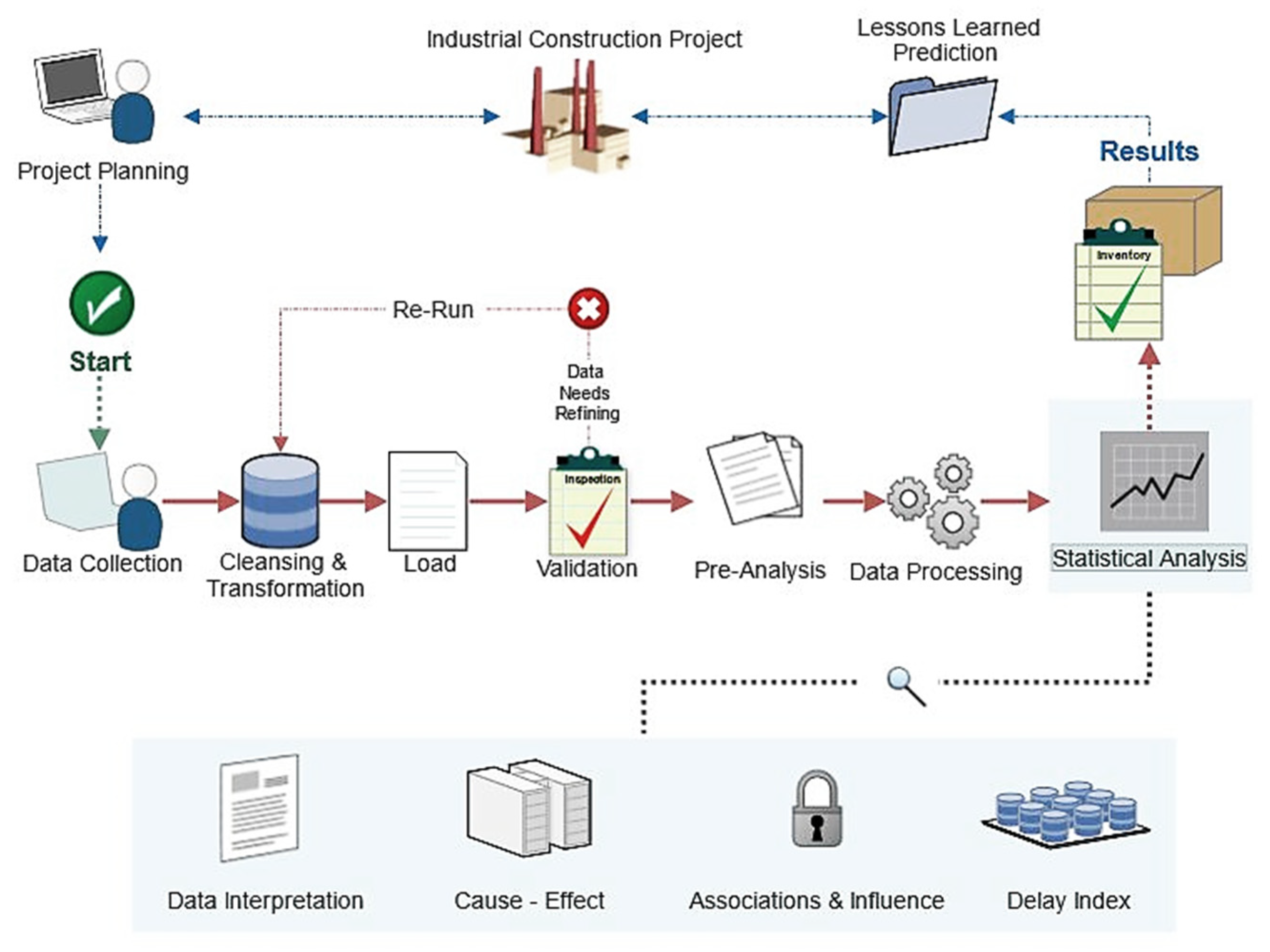
This study focuses on the relationships between and effects of the most important factors (System, Discipline, Specialty, Component) of these projects, and the influence which delays in predecessor activities can have on delays in successive activities. It also examines how to connect delays to the different components of a project at the planning level, starting with the most generic ones such as Systems and moving on to the disaggregated ones such as units or equipment. The aim is not to analyze project delays in general but rather to determine which activities and types of activities tend to experience execution delays during a project, considering the activities, dates, durations, relationships (unique predecessor/successor), and the different elements involved in the planning. The workflow of this approach to the analysis through planning is shown in the
Figure 1.
It is believed that this research could lead to an approach for visualizing certain factors that cause delays in these types of projects and even serve as an analysis methodology if properly developed.
2. Materials and Methods
2.1. Data Collection
For the development of the study, hypothetical data from industrial project plannings were used as a starting point, based on and consistent with real projects, treating the information generically and focusing mainly on basic parameters such as the duration of activities and delays, the relationships between activities (predecessor/successor) and the different components and equipment included in each plan. The projects considered were quite heterogeneous in terms of their scope of application, resources, etc. Nevertheless, they were considered to be representative of the industrial construction field since they shared at least the following common characteristics:
They would be part of an EPC-type contract.
They would be subject to planning and a control and monitoring schedule.
They would include activities such as:
- -
Engineering: basic, detailed, Construction and Commissioning support.
- -
Procurement: equipment and material purchases, manufacturing, supply.
- -
Construction: civil, electrical, instrumentation and control (I&C), mechanical.
- -
Commissioning and Start-up.
There were unique relationships between activities.
2.2. Data Cleansing and Transformation
The first step was to prepare the information from the source data. Given the variety of industrial construction projects that exist, there may be different original data formats (software/PDF/spreadsheet), so they had to be converted to a common format. The medium used to contain and prepare the data before loading them into the statistical software was a spreadsheet.
Although it was possible to perform these tasks in the software itself, before the data were imported, they were cleansed of errors and inconsistent values, removing the parameters that were not going to be used in the study. Other parameters were used instead, such as:
Difference in duration of activities (initial phase/advanced phase).
Delay in the start and finish of an activity (difference of initial/advanced phase).
Delay of the predecessor activity.
This last parameter was of utmost importance, as it tells how an activity was impacted by a predecessor (or predecessors). Once the format had been standardized, the next process was the identification and grouping of:
Systems: associating similar terms to the extent possible.
Disciplines: Procurement, Engineering, Construction, among others.
Specialties: according to EPC scheme; Civil, Electrical, I&C, Mechanical.
Components: basic units or elements of the Systems.
In many cases, the classifications were determined by the planning structure and type of project; in others, the most general criteria possible were assumed in order to identify under which heading various activities or components were included. Within Systems, the main ones and equipment were considered while the rest were included in sections that were as generic as possible in order to cover the diversity of components contained in the plannings.
Since the time interval between plannings is not the same for every project, weighted magnitudes were calculated from the existing data in order to obtain a more harmonized criterion for the values of the study variables. The word “Weighted” was added to these new magnitudes to differentiate them from the original ones.
2.3. Data Import into R
R-Commander, a graphical interface that covers a majority of the most common statistical analyses in drop-down menus without the need to write code, was used for statistical analysis and the creation of graphs, in conjunction with R-Studio, an integrated development environment for the free programming language R [
47,
51,
52].
The data were loaded by choosing the option “Import data set” in the menu, Data→Import Data→From Excel. After the import, the software itself established the qualitative and quantitative variables, which were called factors and variables in this software, respectively, the most significant of these being:
{6} “System”, {7} “Specialty”, {8} “Discipline”, {9} “Component” for factors.
{15} “Delay Start”, {17} “Delay Finish”, {19} “Duration Difference”, {21} “Delay Predecessor” for variables.
The factors were chosen by selecting those that better define the structure of the data set since they were widely present in these types of projects, which benefits the homogenization of the original data and then obtaining results common to the majority of industrial construction projects. Although not listed above, there are other less relevant factors, such as “Project Type”, “Project”, “ID_Activity”, “ID_Predecessor” and “Activity_Name”, rarely used. The description of the variables was as follows:
Delay Start: difference between the planned start date of the planning activity and the actual start date, measured in days. Data is obtained from each schedule.
Delay Finish: difference between the planned finish date of the planning activity and the actual finish date, measured in days.
Duration Difference: difference between the expected duration of an activity and the actual duration, measured in days.
Delay Predecessor: expected end date of the activity preceding the activity and its actual end date, measured in days. The purpose of considering this variable is to try to evaluate the influence that the delay of the activity has on the subsequent one.
What was intended by focusing on the variables chosen was to reduce the number of elements to handle in the analysis to the lowest possible. In this way, instead of working with many variables, only a few were used that group most of the information, simplifying the analysis of the planning. This also allowed for generating other variables if necessary, as done with the weighted ones, which were calculated by dividing the variable by the duration in months of the project.
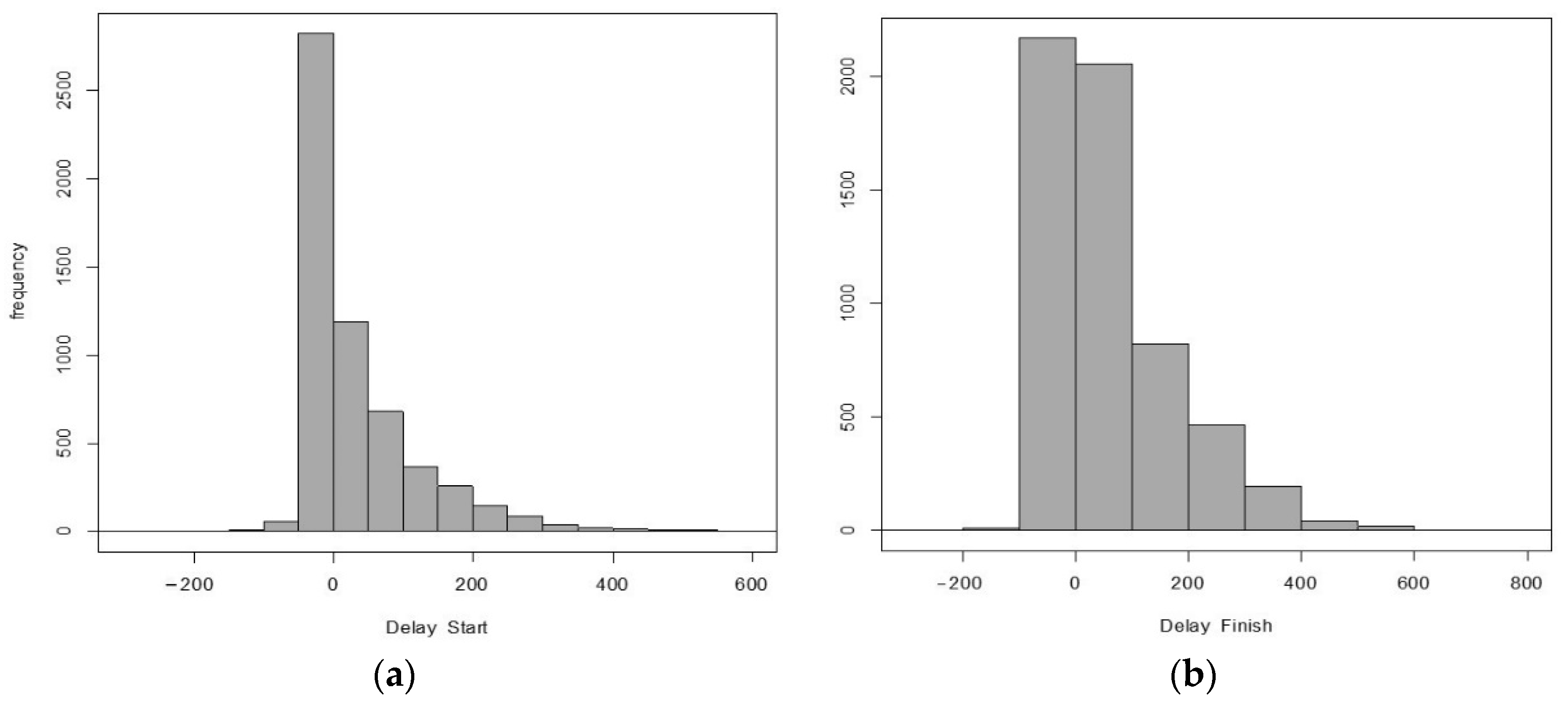
The first verification was a summary of the active data set from Statistics→Summaries→Active data set. The general information of the data set comprised a total of 6216 entries corresponding to five projects, including minimum and maximum values, first and third quartiles, the median, the mean, and the missing values. The same summary showed the frequency distribution of the main items in each category.
One important piece of information that this initial analysis revealed was the dispersion of data and the existence of many missing values in relation to the delays in the start and finish of the activities. It can also be seen that these were left-skewed asymmetric distributions of values where the mean was greater than the median, as shown in the
Figure 2. This can also be seen in the Numerical Summaries of the variables, such as the one for “Delay Finish” and “Duration Difference”, where the dispersion measurements extracted using the menu option Statistics→Summaries→Numerical summaries can be visualized.
The next step was to apply filters to reduce anomalies that could be due to issues not directly related to the execution of the project itself (force majeure, financial problems, onsite risks, etc.), and to limit existing outliers given the dispersion of data. At the same time, possible errors were minimized using statistics and inference. Following an iterative process to estimate the best fit, the filtering for “Delay Finish Weighted” was performed for values 30 > X > −10, while for “Duration Difference Weighted”, filtering was performed for the interval 30 > X > −10. The final number of rows compared to the spreadsheet dropped from 6216 to 5145, with the total number of activities decreasing by 17.2%. A new overview of the active dataset was then generated, summarized in the
Table 1, which showed minimum delay values reduction.
2.4. Statistical Analysis
Once the data set was configured, different statistical studies were carried out. First, a more detailed summary of the new set was drafted as the starting point for the analysis from a descriptive point of view, with statistics for the complete set. Then, the key characteristics of the duration and delay variables were reviewed in order to describe them using a small number of descriptors. This exercise helped to visualize trends and to summarize and characterize data and interpret them. The key conclusions of this section showed:
A (persisting) lack of uniformity of the factors under study in the dataset and the dispersion of variable values.
A reduction in the average duration of activities as the project progresses.
Shorter delays in completing activities in the advanced stages than at the start.
For this summary, it was started with the options in Statistics→Summaries→Numerical summaries to evaluate the centrality and dispersion of the variables and the effectiveness of the filter applied to reduce outliers, relying on the graphs available in the Graphs menu:
Statistics: frequency tables and numerical characteristics of position, centrality, and dispersion such as mean, median, maximum, and minimum, quartiles, or skewness.
Graphs: scatterplots and plots of means which facilitate the transmission and presentation of information in a visual way.
The next step was the comparison of variables and correlation using the different options in the Statistics→Summaries menu, where associations between variables and factors are checked using:
This was used to check the relationship between different variables in order to determine the existence of a cause-effect relationship. The following conclusions were drawn from the results obtained, among others:
The farther along with in the phases of a project, the greater the delay by Discipline.
There was a direct relationship between a delay in predecessor activity and a delay in the completion date of the next activity.
As an example of possible combinations for segregating information in this and subsequent sections, the data was usually filtered for Construction Discipline, Mechanical Specialty, or a combination of both, or Engineering and Civil.
Linear regression analyses were then conducted to determine the function that interprets the relationship between the dependent and the independent variables. In addition to providing information on the residuals, the results were used to obtain the coefficient of determination, R
2, which allowed for studying the goodness-of-fit of the model, as well as the values of the test statistics and the corresponding
p-values [
53] in the following cases:
Single, between predecessor and successor.
Two-degree, predecessor-successor-subsuccessor: the relationships between an activity, its successor, and the successor’s successor must be established.
Multiple, with grouping by factors.
The key conclusions of this section were as follows:
As the delay in the predecessor activity increases, the delay in the activity under review increases.
The duration of an activity increases in direct relation to a delay in the Finish date.
The more distant the degree of relationship between activities, the smaller the effect which the delay of the predecessor has on the subsequent successor.
No conclusive results can be drawn on the impact of second-degree successor activities or the multiple linear regression developed.
With regard to the analysis of variance to assess the differences in delay per project, it was considered that there were significant statistical differences between them, either in general or those of the PXE type.
Finally, it was concluded by determining the Components with the greatest completion delays and their relationships with the following stages. To that end, a new parameter called Delay Index was defined, which was calculated using median values and the interquartile range (IQR), finding that the main activities related to the elements considered in this index were the ones concerning Mechanical Insulation and one type of Turbine. When the predecessor activities of this Turbine were analyzed, it was observed that Mechanical Supply activities as those with the highest incidence.
3. Results
3.1. Descriptive Analysis
Given the high number of factors and variables, only some of the cases were shown in this section. For the descriptive analysis, a summary of the active data set was created to calculate basic statistics for these factors and variables. The information of some of the main factors is shown in the
Table 2 below:
What was observed was a lack of uniformity of the data in terms of the Specialty and Discipline factors, as was to be expected due to the different types of input data.
A summary was obtained for each of the variables in order to begin assessing the centrality and dispersion of these variables and to draw initial conclusions. In the case of the evolution of the durations and delays of the
Table 3, it seemed clear that as the stages of the project advance (Design Engineering, Procurement, Construction, Commissioning), the average duration of the activities was reduced, either due to adjustments as the project reaches the final stages or due to the needs of the project to make up for cumulative delays.
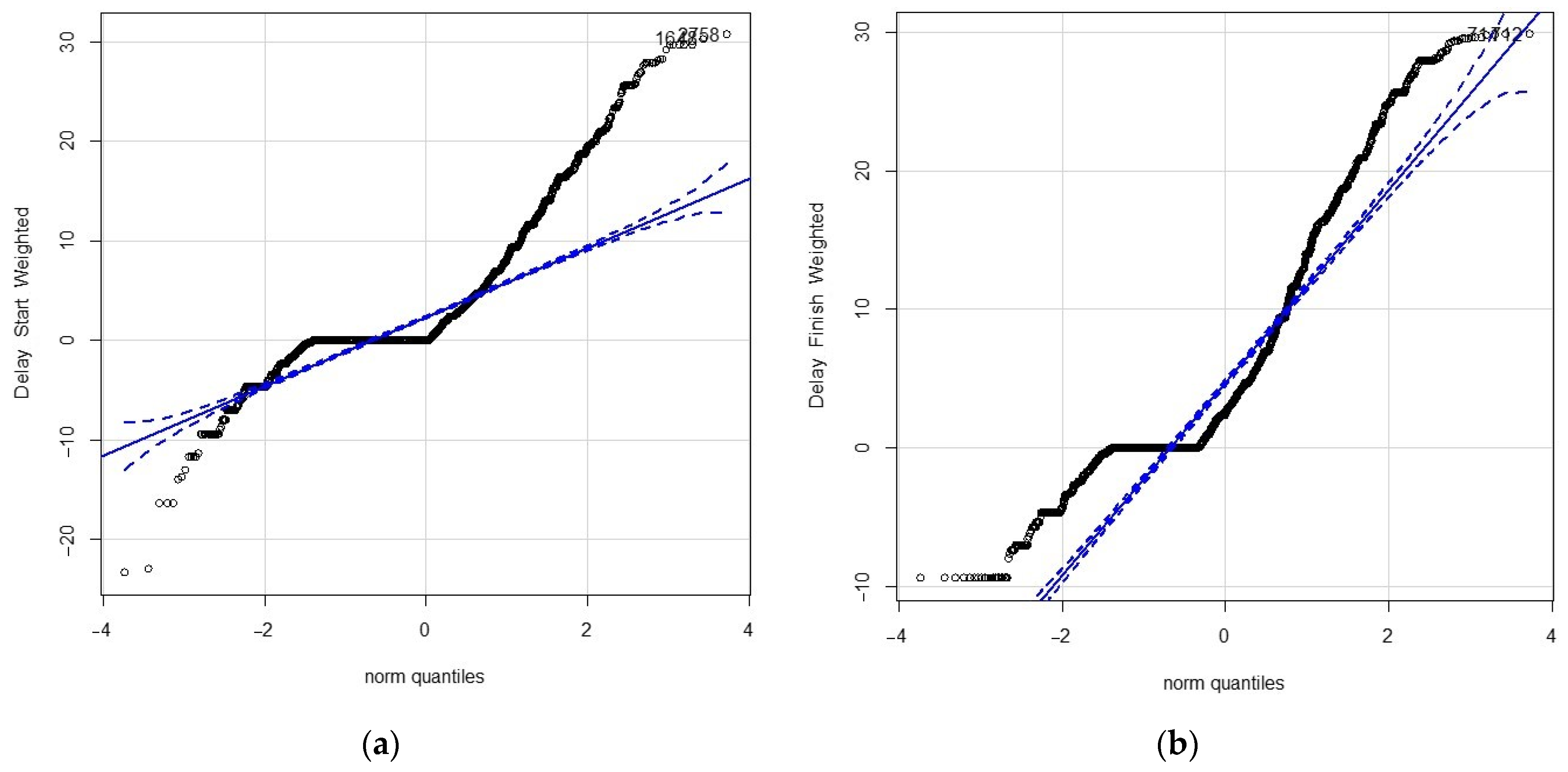
On the other hand, the delay in starting an activity at an advanced stage was less than the delay in finishing. In other words, although there was relatively little delay in starting activities compared to what was planned at the beginning of the project, the delay in completion increased significantly for the cases under study. Add to this the information provided by the percentiles as well as positive skewness with the most extreme values above the mean, and it was confirmed that there was a shift in the delay of activities which was more pronounced for the variable Finish. This is presented in
Figure 3 and
Table 4:
It was also clear from these values that the dispersion of the variables, despite data cleaning and filtering, was still significant and that, in some cases, there were quite a few outliers, which was also visible in the different descriptive analyses.
3.2. Comparison of Variables and Correlation
Contingency tables can be used to infer information on the activities with the greatest relative weight in relation to the factors. Specifically, in the projects analyzed and for the Discipline and Specialty factors, these activities were Procurement and Commissioning within the Mechanical Specialty, with Civil Engineering activities related to the Construction phase also having particular relevance in the projects, as shown in
Table 5. This was consistent with the sector in which industrial construction projects were carried out, where it was common to start from scratch with earth movement for the Civil Engineering and Construction portions and the need for extensive Mechanical equipment to do the work. It was also noteworthy that the importance of Civil Engineering activities disappeared during commissioning, as is logical. As for the general part of the project, the Electrical Specialty was the one that has the greatest influence on the activities.
By way of example, in the case of Systems filtered by the Engineering Discipline, the activities related to I&C were seen to have greater relative weight in Engineering activities than in the rest of the Specialties. This was largely due to the importance of the Distributed Control System (DCS), which was critical to the operation of an industrial plant.
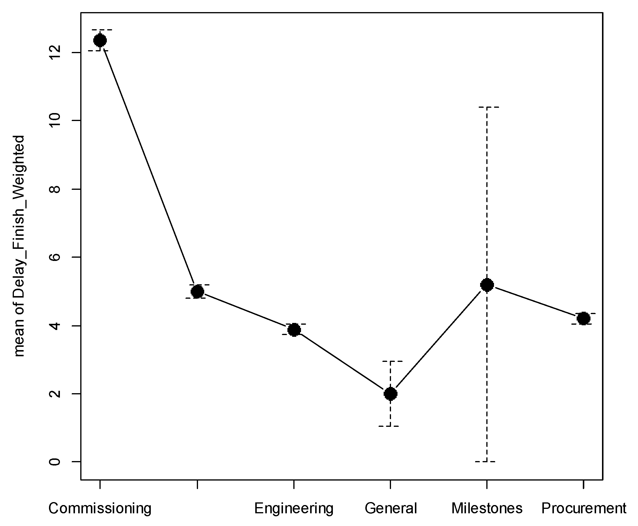
Moving on to other numerical summaries, in the comparison of delays by Discipline, it seemed clear according to
Figure 4, that the delays increase as the project advances through the different phases.
Using the value of the weighted variable in this case, what it showed was that the delay in Engineering < Procurement < Construction < Commissioning, which is in line with the different stages of project development according to the theoretical phases of a construction project of this kind. The same occurs when predecessor activities are analyzed: the further along the project is, the longer the delay.
It was also necessary to verify the relationship between some variables and others, i.e., to discern whether there was indeed a cause-effect relationship that was appreciable from an analytical or statistical point of view. A correlation matrix was used for this purpose.
According to
Table 6, the linear correlation coefficient of Predecessor Delay and Duration Difference was 0.10, a very weak association, but for Delay Finish it was intermediate at 0.55. Another intermediate result, with a value of 0.59, was the correlation between Delay Finish and Duration Difference. In other words, there was a direct relationship between a delay in predecessor activity and the completion of the next one, and thus an increase in the duration of the successor activity.
It was possible to filter using different factors, such as Specialty or Discipline, to see how the different variables behave as the level of detail increased. The delay in the predecessor activity, in the case of Specialty = Mechanical, had a greater impact on the delay of Mechanical activities than on the overall activities. However, when the Mechanical Specialty was observed for Construction activities only, the relationship between the predecessor and the successor activity was somewhat weaker.
All of these statistical analyses provide useful data for similar construction projects. By knowing which activities are critical, it is possible to identify which predecessor activities to focus on in order to improve efficiency and take preventive actions to limit cumulative delays.
3.3. Linear Regression
3.3.1. Delay Finish
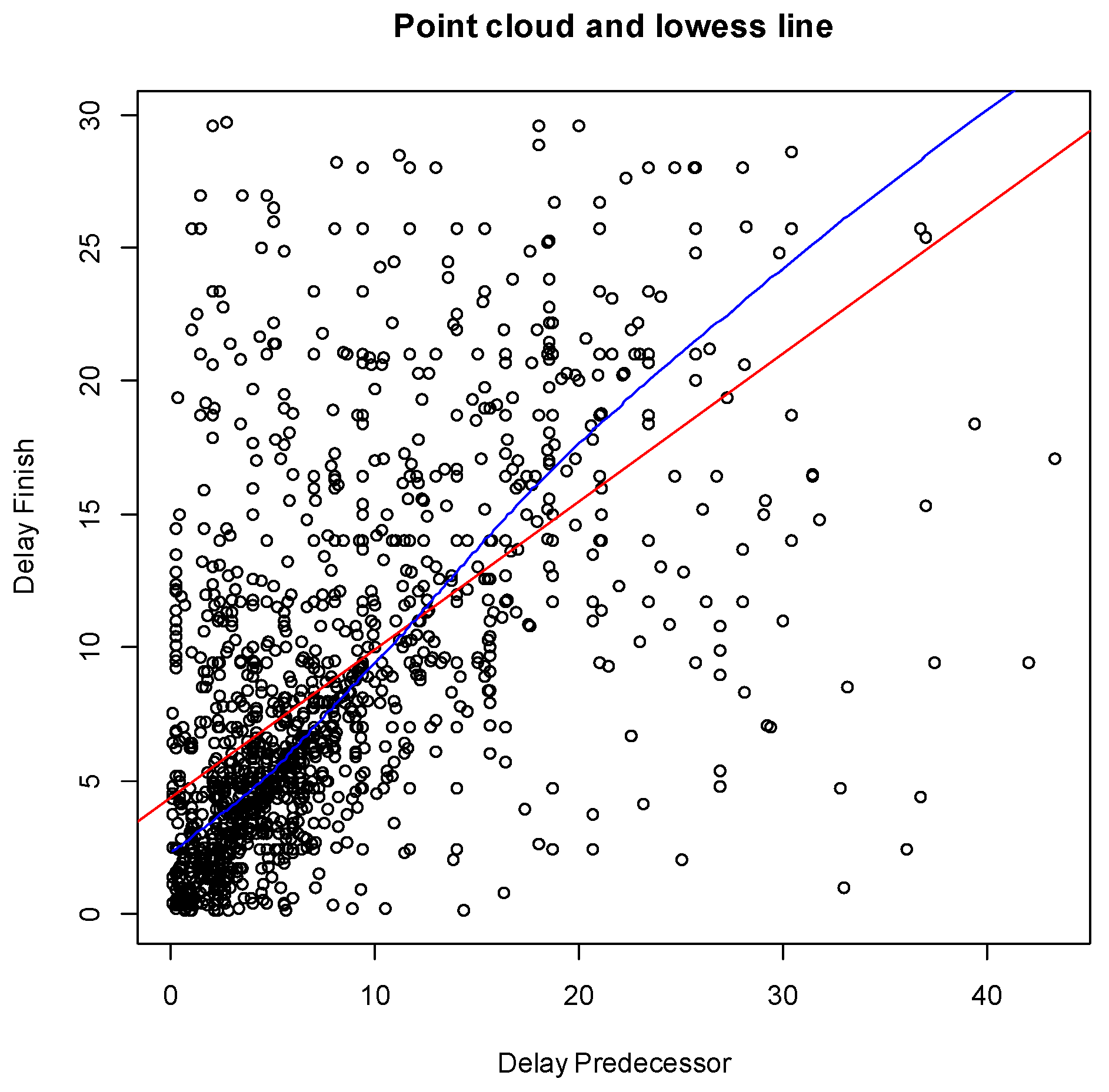
After obtaining the correlation results, the linear regression model was reviewed with respect to the totality of the activities, using Delay Finish in relation to Delay Predecessor as the dependent variable. The following results were obtained with weighted variables as shown in
Table 7. In this model, the
p-values that help to resolve these contrasts were in both cases, 2 × 10
−16, a value less than 0.05 [
54,
55].
Thus, considering a significance level of 5%, the null hypothesis would be rejected in both cases, concluding that there was a linear relationship between the variables. Therefore, as the delay in the predecessor activity increased, the delay also increased and the linear model can be written as follows, considering the model function y = α + βx which describes a line with slope β (i.e., regression coefficient = Delay Predecessor Weighted coefficient) and y-intercept α [
56]:
The smaller the residuals, the better the fit of the model to the data and the more accurate the predictions made using the model, as the residuals are the differences between the observed responses of the explanatory variables and the prediction calculated using the regression function [
57]. The standard error of the residuals indicates the dispersion of the residual values so that the better the fit, the smaller the standard error. In this case, the standard error of the residuals was 5.966.
The value of R
2 (Multiple R-squared) ranged between 0 and 1 [
36,
54], so values close to 1 indicated a good fit of the linear model to the data. In this case, 30.53% of all variability related to the delay in the completion of Mechanical Construction activities can be explained by the delay of the predecessor.
The model, fitted to the point cloud with the addition of a smoothed lowess line [
58], is plotted in
Figure 5. All data must be positive in order to obtain such a lowess line, so the data table was transformed to positive by filtering for Delay Predecessor Weighted and Delay Finish Weighted >0. In addition, it was filtered by Specialty for this example.
In the case of the Duration Difference weighted variables explained by Delay Finish, the
p-values were also less than 0.05, so there was a linear relationship between the variables, as stated in
Table 8.
Although the descriptive section concluded that, in general, activities tended to get shorter as the project progresses, the regression also showed that the duration of activities whose completion date had been delayed increases, despite the fact that corrective measures should be taken to compensate for the delay caused by reducing the duration of the activity:
3.3.2. Delay with Two-Variable Filtering
To evaluate the option of obtaining a higher level of detail in the results, different estimations of linear regression models were performed by changing the variables. In another representation, shown in
Table 9, the regression was again filtered, as in the previous sections, by Construction and Mechanical to check the behavior of the model.
The
p-values were 3.13 × 10
−14 and 2 × 10
−16, meaning that in this case, the impact of predecessor activities was lower than in the general case, 28.43%, obtaining the following linear model:
There were numerous possibilities and combinations. Depending on the variables, different filters can be applied to obtain the results that allowed them to be properly analyzed.
3.3.3. Impact on Successive Activities
Linear regressions between the predecessor (0) of an activity (I) and the delay in the completion of its successor (II) were also evaluated. For activities where the predecessor was an activity in the Engineering Discipline and the Mechanical Specialty, it was found that the variability of the delay in the completion of the successor II activity was only due to the initial predecessor 11.98% of the time, as can be seen in
Table 10. It followed that the more distant the relationship between activities, the smaller the effect which the delay of the predecessor had on the subsequent successor (II). However, as more filters were applied and the level of detail increased, the null hypothesis cannot always be discarded.
In the case of Mechanical Engineering on the table above (Mech. Engineering & Cons), it does not have a significant effect on second-degree Construction activities, while in the case of the impact of Civil Engineering on the Construction subsequent successors (Civil Engineering & Cons), this conclusion is not as obvious since the p-values are bordering on the acceptable limit.
3.3.4. Multiple Linear Regression
The next observation refers to the development of a multiple regression model. It contains more than one independent or explanatory variable, which could even be qualitative (factor), and which determines the value of the variable to be analyzed. The effect of a predecessor activity, segmented by Discipline, on the completion of the second-degree successor activity (subsuccessor) is studied and shown in
Table 11.
Looking at the p-values, only delays in the Commissioning predecessor and, to a lesser extent, Milestones, seemed to have an influence on the delay of the subsuccessor, but the number of observations within the dataset was very low (around 2.1%), so this kind of analysis did not appear to yield conclusive results.
3.4. One-Way Analysis of Variance (ANOVA)
This analysis of variance made it possible to compare different groups in relation to a variable. In the case shown in the
Table 12, the different projects in the study (factor) were compared with respect to the delay in the completion of activities (variable).
The groups to be compared should be normally distributed and homogeneous, but because they were large in size it was less important to ensure these two assumptions since ANOVA is usually a fairly “robust” technique, behaving well with respect to transgressions of normality [
59,
60]. The corresponding hypotheses are:
Hypothesis 1 (H1). The delay in the completion of activities is the same in all projects.
Hypothesis 2 (H2). Some are different (there are differences between at least some of the five projects).
According to the data obtained in the table above, the mean delays in the completion of activities differed. It can therefore be concluded that there were statistically significant differences between the projects with respect to the delay variable, since F(4.5140) = 274.3 (not equal to 1), with
p < 0.05 (2 × 10
−16) [
54,
61]. This was the expected result, given the non-uniform nature of the projects and their source data.
The same was true for PXE-type projects where, as shown in
Table 13 and despite similarities, there were significant differences in the magnitude of the delays in general and for the Disciplines in particular. In the latter case, the F-value was lower than before, but far from a value of 1.0.
This type of analysis was useful for evaluating the projects for which it was appropriate to work with statistically more homogeneous parameters when the information was to be included in a dataset to be studied.
3.5. Component Lag Analysis
To conclude the statistical analyses, a new numerical summary was carried out to calculate the mean and standard deviation values of the delays in the completion of the activities for equipment, materials, etc., under the Components heading of the data table. The median was also extracted for each one. Since they were widely dispersed values, it was quite indicative of the ones that need to be reviewed.
Given that the average variation between the mean and the median of the weighted lag variable per element yielded a value of 69.07%, the latter was used along with the interquartile range (IQR) to determine the Components with the highest lag index.
The IQR interquartile range was the difference between the third and first quartiles to estimate the dispersion of data distribution, highly recommended when the measure of central tendency used was the median. Considering that the total number of rows was 5145 with 96 types of Components, those with a frequency of occurrence of at least half the average, i.e., 26.80, were evaluated:
obtaining the ranking by index on
Table 14, where the activities related to Insulation and Turbine A would have the highest rate of delay:
However, not every activity has a predecessor and they are not always homogeneous even if they do exist. By way of example, also presented in
Table 15, using the source data on the spreadsheet, for Turbine A, there were various types of predecessor activities. These ranged from Procurement activities for the Turbine itself (6 Procurement and 2 Supply-related) to lifting elements in the case of the Crane System in the Construction Discipline. The Specialties were Civil, Electrical, Mechanical and one General which corresponds to Basic Engineering.
From there, it became possible to establish criteria for relationships and the possibility of examining the impact of each predecessor on successive Turbine activities. Successive analyses can be carried out, e.g., how each predecessor activity by Discipline (or System or Specialty) influences the cumulative delay of other activities, either in absolute or relative terms, weighted values, as a percentage or other metrics suitable for quantifying and evaluating such influence.
Table 16 shows the average impact of the delay in a predecessor activity on the completion of DCS activities by Discipline.
4. Discussion
The analysis of planning is a tool that can be used to identify key points affecting the development and efficiency of industrial construction projects, as the amount of information and lessons learned that can be obtained are significant. However, the level of digitization of these types of projects remains low, which is a major handicap for management and control, as well as for subsequent diagnosis. It is also one of the reasons for the productivity gap compared to other industrial sectors [
62].
In this study, the use of advanced statistical software for data analysis was examined as a way of contributing to closing this gap and to assess the suitability of its use as part of a methodology that can lead to more effective identification of the elements and causes of delays during the execution phase, based on the study of scheduled activities.
It was possible to extract relevant information from these plannings in a fast and effective way, demonstrating the ease of use of the chosen interface and showing the multiple possibilities it can offer, although statistical knowledge is necessary to take actions or interpret results. In addition, programming is required for options not currently included in the menus, but the capacity and, above all, the speed of calculation allowed complex and repetitive operations to be carried out in a relatively short period of time.
As a starting point for the work, the task of extracting and standardizing project data from different areas was an arduous one, so the possibility of automating this process would be a substantial improvement. This is where the development of new technologies can play an important role, both in the initial phases of extracting common information (relating concepts) and later in the transformation of data before loading it for subsequent analysis using data mining, Big Data, or machine learning tools. The use of automation routines would simplify work time, providing continuous, reproducible, and repeatable analysis, while reducing errors.
Regarding the actual development of the study, descriptive analysis was used to define the characteristics of the data set for the study and to assess the dispersion of its components using a small number of descriptive statistics. The results showed there was a need to homogenize the data and eliminate anomalies in order to extract more conclusive results. This task was performed using filters and establishing new weighted variables. The initial analysis showed that there was still a lack of uniformity of the factors in the data set and dispersion of the values of the variables. This first analysis also served as the basis for representing trends and for summarizing and characterizing data on the variables relating to the duration and delays of planning activities as the different phases of the projects progressed.
It was subsequently possible to deepen the analysis through the use of variable comparison and correlation tools. It was observed that as the project advanced through the different stages there was a greater incidence in the delays of activities with respect to the original project planning. To a large extent, this was caused by delays in predecessor activities, as a consequence of which the completion date of the next planned activity was shifted.
Linear regression showed that those activities whose completion dates were delayed also experienced an increase in duration so that the delay has a dual effect. It was also found that the more distant the degree of relationship between activities, the smaller the effect which the delay of the predecessor has on the subsequent successor. However, it was not possible to draw conclusive results regarding the impact of second-degree successor activities in all the combinations of Specialties/Disciplines or from the multiple linear regression carried out, either because of the low number of observations available in the dataset or due to the statistical parameters which were bordering on the acceptable limit.
Regarding the analysis of variance, the key conclusion is that this type of analysis offers the possibility of determining the projects whose parameters are statistically more homogeneous, in order to choose the most similar projects and extrapolate the results to others with comparable characteristics.
When evaluating the causes of delay by Component, the establishment of the “Index” parameter made it possible to identify those components with the highest rate of delay. From there, it was possible to determine which activities influenced their behavior and the impact on the activities with which each Component was directly related.
Regarding the aspects not addressed in the study, it would be feasible, although more complex, to expand it so that each activity would have more than one dependency (predecessor activity). This would also be subject to availability in the source data but would increase the options and the capacity to generate usable results. As the quality and quantity of the source data increases, so does the refinement of the model in relation to sub-successor activities, which in the study were found to be insignificant (
Section 3.3.3).
As far as planning is concerned, although no tool of this kind was reviewed in this study, the use of new tools in the construction sector such as 4D software, which combines three-dimensional systems with time as a fourth dimension, is becoming widespread. Among the advantages of 4D software are the increased efficiency in the planning process of construction projects and more efficient monitoring and control of progress [
63]. The use of 4D software adapted to the field of industrial projects which provides the required level of planning detail would mean that there would be much more available data and relationships between activities, leading to a much more robust model. Furthermore, as part of the process of digitizing the industrial projects sector, it is expected that the development of new technologies will provide new tools that will improve the efficiency of complex construction projects and increase the information available for analysis, such as advances in the field of Artificial Intelligence (AI) planning or the use of BIM [
64,
65,
66,
67].
5. Conclusions
This study presented an approach based on a planning analysis methodology to assess the certain elements that can influence variations in execution times during the development of construction industrial projects, and to identify, to the extent possible, those components that are most significant in this respect using different techniques, as well as the impact in other components, considering the activities, dates, durations, relationships and the different elements part of the project schedules.
As part of the conclusions of this initial phase of the analysis, it was concluded that with this methodology, it was possible to determine the Specialties, Disciplines, and Systems whose activities had more influence on the rest of the factors. In the case of Specialties:
Mechanical activities were almost 54% of Commissioning, 38% of Engineering, and above 56% of Procurement,
Civil activities represent more than 38% of Construction.
This basic evidence from planning can provide the projects with operational information to define the necessary resources leading to an efficient development of the projects. Other information available from this data—which are also useful for other projects—are related to the Systems with the greatest relative weight in Disciplines. Although the Specialties of the Systems are varied, still the outstanding influence of the Mechanical part can be found, being the more relevant Systems for Commissioning, the turbines A and B and boiler; civil works, power source installation and water systems for Construction; electrical system, mechanical assembly and civil works for Engineering; electrical and mechanical systems for Procurement.
As stated before, by identifying the critical activities it is possible to focus on predecessor activities in order to improve efficiency and take preventive actions to limit cumulative delays. The lag in the predecessor activity had a greater impact on the delay of Mechanical Specialty than in I&C, with a similar effect in Electrical, while the Civil Specialty presented the lower ratio according to the results.
Linear regression was conducted to determine the function that interprets the relationship between the dependent and the independent variables in different cases, from single to multiple linear regression. The key conclusions of this section are as follows:
The linear regression equations established that the delay of activity increases its duration and is directly proportional to its predecessor.
The more distant the degree of relationship between activities, the smaller the effect which the delay of the predecessor has on the subsequent successor.
For instance, in activities where the predecessor was an activity in the Mechanical Specialty, the most influent one according to the contingency tables, the variability of the delay in the completion of the second-degree successor as a result of the first predecessor is reduced up to three times compared to the direct case. Based on this knowledge, it is possible to predict and control those activities with a higher probability of affecting other elements.
As a final point, the use of the component lag analysis Index was found valid to specifically determine the Components with the highest delay occurrence. In this particular case, it is reflected again the importance of Mechanical activities and components (insulation, turbines, valves).
In relation to the limitations, firstly, the data is based on and in general consistent with real projects, but some information and results could be considered as inexact due to that nature. The aim is to focus on the feasibility of using this methodology rather than considering the contributions of the numerical results. The use of statistical software facilitates the capture of valuable information for organizations. However, it is worth noting that in order to refine the model and be able to extrapolate the results to the industrial projects sector, it would be advisable to study a larger number of plans. As indicated above, the international procurement market was worth
$7.60 trillion at the end of 2019 for EPC projects [
7]. Without distinguishing between fields and assuming an average price of
$400 million per contract, the number of projects would be somewhere around 19,000. With a confidence level of 95% and a margin of error of 5%, a sample of at least 379 projects would be required. For a 90% confidence level and a 10% margin of error, data from at least 68 of these projects would be required.
At the same time, the wide variety of sectors where industrial projects are carried out conditions the extrapolation of findings from one project to another, not only by segment but also by company.
Finally, it was noted that there are multiple possibilities and combinations for studying variables and that different filters can be applied to refine the study of these variables. However, as these filters are applied, the amount of data is reduced, so the results were not found to be relevant to the case study. Something similar happens with multiple linear regression, where the scarce number of observations available did not allow the quantitative results to be considered conclusive, beyond the validity of the methodology itself.


