Spatiotemporal Change and Coordinated Development Analysis of “Population-Society-Economy-Resource-Ecology-Environment” in the Jing-Jin-Ji Urban Agglomeration from 2000 to 2015

Abstract

Measuring the regionally coordinated development degree quantitively at an urban agglomeration scale is vital for regional sustainable development. To date, existing studies mainly utilized statistical data to analyze coordinated development degrees between different subsystems, which failed to measure the development gap of subsystems between cities. This study integrated remote sensing and statistical data to evaluate the development degree from six subsystems. The coordinated index (CI) and coordinated development index (CDI) were then promoted to assess the coordinated degree and coordinated development degree. The main findings were: (1) The coordinated development degree of Jing-Jin-Ji (JJJ) had increased from 0.4616 in 2000 to 0.6099 in 2015, with the corresponding grade improvement from “moderate” to “good”; (2) JJJ and six subsystems’ development degree showed an increasing trend. JJJ’s whole development degree had improved from 0.34 to 0.52, and the grade had changed from “fair” to “moderate”; (3) The coordinated degree of JJJ displayed a “V” shape. However, the coordinated degree was lower in 2015 than in 2000.

1. Introduction

Since the implementation of the reform and opening-up policy in 1978, tremendous changes have occurred in mainland China [1,2]. However, accompanied by a high economic growth speed, several problems have arisen, such as a low resource utilization efficiency, a high degree of environmental pollution, a wider economic development gap, etc. In response to these problems, the Chinese government promulgated the regional coordinated development strategy in 2017. To date, numerous studies have focused on this topic. Specifically, from the point of view of definition, it could be divided into two types. The first one refers to the synchronized development of different subsystems. These subsystems included population, society, economy, environment, etc. For instance, Li and Yi assessed the city’s coordinated development level from three subsystems, which were economy, society, and environment [3]; Xie et al. analyzed the coordinated development of the “resources-environment-ecology-economy-society” complex system in China [4]. The second one refers to the economic gap narrowing between different regions. For example, Qin et al. evaluated China’s economic gap and its coordinated development level [5]. However, both definitions consider one-sided aspects of development. The first one emphasized the synchronism of various subsystems but failed to assess each subsystem’s gap between regions. The second one only measured the regional economic gap while ignoring other subsystems, such as population, society, resources, etc. From a methodological point of view, these studies can be grouped into three types: the development degree model, the coordinated degree model, and the coordinated development degree model. The first type includes the principal component analysis (PCA); for instance, Bolcárová and Kološta [6]. The second type includes grey relational analysis [7], data envelopment analysis [8], system dynamic analysis [9], etc. The third type includes the coupling coordinated degree model (CCD) [10,11]. For example, Lin et al. evaluated the coupling coordination changes between the urbanization quality and eco-environment pressure of the West Taiwan Strait urban agglomeration [12]. Li et al. assessed the coordinated development between social economy and ecological environment in northeastern China [13]. Fan et al. studied the coupling coordinated development situation between social economy and ecological environment in Chinese provincial capital cities [14]. In general, these studies measured mainly the coordinated development degree under the first definition. As for data sources, traditional research mainly applied statistical data to evaluate the coordinated development degree. For instance, Zameer et al. investigated the coordinated development of natural resources, financial development, and ecological efficiency in China [15]; Zhang et al. used panel data to assess the development level of the “Five Modernizations” [16]; Ma et al. utilized statistical data to evaluate the coordinated development from the perspective of new urbanization [17]. Generally, statistical data have their advantages, like high authority and accuracy; however, they also have some disadvantages, such as the inconsistent statistical caliber, limited coverage, and incomplete statistical indicators. Compared with statistical data, non-statistical data have been gradually utilized to investigate the regionally coordinated development degree. For example, Ariken et al. evaluated the coordinated development degree of urbanization and eco-environment in Yanqi Basin based on multi-source remote sensing data [18]; Tian et al. combined land use data and statistical data to analyze the coordination state between urbanization and ecosystem services [19]; Yang et al. integrated spatial data, environmental data, and statistical data to evaluate the coupling coordination of geo-ecological environment and urbanization [20]; Shao et al. explored the relationship between urbanization and ecological environment using remote sensing images and statistical data [21]. Based on these studies, we found that remote sensing data were gradually applied to evaluate the ecological quality. However, due to the ecology subsystem’s complexity, numerous studies mainly assessed one aspect of it [22]. In this context, one comprehensive index, named remote sensing ecological index (RSEI), was promoted by Xu in 2013 [23]. Since its promotion, this index has been widely applied in numerous studies; however, it was seldom applied to assess the ecological quality at a large scale due to some limitations, like the difficulty of obtaining the same period’s data and cloud pollution [24]. Integrated with MODIS datasets and Google Earth Engine technologies, Ji et al. successfully evaluated the regional ecological quality at an urban agglomeration scale [24,25].

As for the weighting methods, existing studies could be divided into subjective weighting methods, such as the analytic hierarchy process (AHP) [4,26,27] and the Delphi method [28], objective weighting methods, such as global principal component analysis [29] and the entropy method (EM) [30,31,32,33,34,35], and combined weighting methods, such as the fuzzy analytical hierarchy process (FAHP) and the entropy method [36,37]. In general, subjective weighting methods have the advantage of considering the expert’s experience while ignoring the information of the data themselves. On the contrary, objective weighting methods consider the data’s information while ignoring the decision makers’ subjective intentions. Combined weighting methods utilize the advantages of both subjective and objective weighting methods, which have become more and more popular. Regarding the subsystems’ selection, we concluded that population, economy, society, resource, ecology, and environment were the primary subsystems [38,39,40,41,42,43]. However, due to the similarity between environmental and ecological concepts, both subsystems’ selected indicators were also similar [11,36]. The concept of environment mainly refers to the interaction between human beings and their living environment, while ecology mainly refers to the natural ecological situation.

Based on the above literature review, we first defined the regional coordinated development as “Within a certain geographical space, the internal development level of its population, society, economy, resource, ecology, as well as environment tend to improve, and the internal differences tend to narrow, thus moving forward as a whole.” Then, we constructed the indicator system from six subsystems: population, society, economy, resource, ecology, and environment, and assigned each subsystem’s weight by combining AHP and EM. Finally, we introduced one novel coordinated index (CI) and calculated the coordinated development index (CDI) to analyze Jing-Jin-Ji’s (JJJ) changes during 2000–2015. This paper is organized into five sections. The first section introduces the background of the study and its rationale. The material and methods section introduces the study area, the data source and indicator calculation, the acquisition of combined weighting, and the CI and CDI calculation. The result section incorporates the development degree and coordinated degree of JJJ and each subsystem in different years. The discussion part explains the weight allocation result, cause analysis, implications, and limitations of the study. The last section represents the conclusion of the study.

2. Materials and Methods

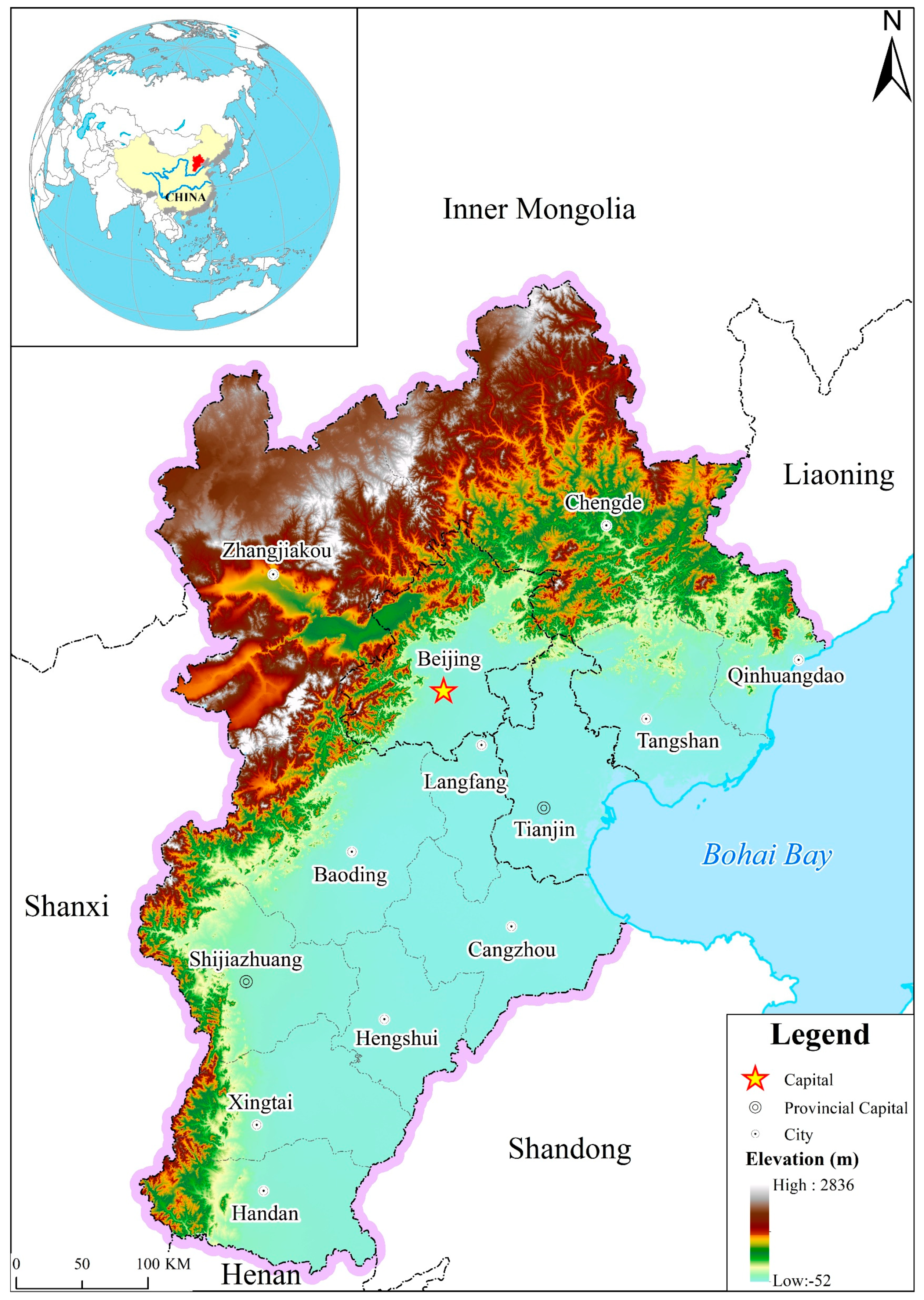
2.1. Study Area

The JJJ urban agglomeration is located in northern China, covering approximately 218,000 km² (Figure 1). It has a total of 13 cities with different categories. Beijing (BJ) and Tianjin (TJ) are municipalities, while Shijiazhuang (SJZ), Tangshan (TS), Qinhuangdao (QHD), Handan (HD), Xingtai (XT), Baoding (BD), Zhangjiakou (ZJK), Chengde (CD), Cangzhou (CZ), Langfang (LF), and Hengshui (HS) are prefecture-level cities. As one of China’s three economic growth engines in the 21st century, JJJ’s further development could contribute a lot to China’s growth. In 2019, the total population and GDP reached 113.07 million people and 8458.00 billion yuan, accounting for 8.10% and 8.54% of the country’s overall values.

2.2. Indicator System and Data Collection

Based on the literature [3,4,5,6,7,8,9,10,11,12,13,14,15,16,17,18,19,20,21,26,27,28,29,30,31,32,33,34,35,36,37,38,39,40,41,42,43], we have collected 232 indicators at the beginning. Then, correlation analyses were done to exclude indicators with a high correlation coefficient. Finally, 25 indicators were selected based on the principles of comparability, accessibility, representativeness, and computability (

Table 1. Indicator system.

Subsystems	Attributes	Indicators	Unit	Trend	Data Source
Population	Population quantity	Total resident population (C1)	10,000 person	Negative	(1)(2)(3)(4)
	Population structure	Proportion of employees in the tertiary industry (C2)	%	Positive	(1)(2)(3)(4)
		Proportion of the urban population (C3)	%	Positive	(1)(2)(3)(4)
	Education level	Per capita of years of education (C4)	Year	Positive	(2)(3)(4)(5)(6)
Society	Infrastructure construction level	Number of mobile phone users per 100 people (C5)	Users	Positive	(1)(2)(3)(4)
		Per capita built-up area (C6)	m2	Positive	(1)(2)(3)(4)
		Road density (C7)	m/km2	Positive	(7)
	Basic public service level	Number of doctors per 10,000 people (C8)	People	Positive	(1)(2)(3)(4)
		Number of beds in hospitals and health centers per 10,000 people (C9)	Unit	Positive	(1)(2)(3)(4)
		Number of buses and trams per 10,000 people (C10)	Unit	Positive	(1)(2)(3)(4)
		Number of full-time teachers in universities per 10,000 people (C11)	Person	Positive	(1)(2)(3)(4)
		Number of books in public libraries per 100 people (C12)	Unit	Positive	(1)(2)(3)(4)
		Proportion of basic medical insurance (C13)	%	Positive	(1)(2)(3)(4)
Economy	Economic quantity	GDP (C14)	Billion yuan	Positive	(1)(2)(3)(4)
		Per capita GDP (C15)	Yuan	Positive	(1)(2)(3)(4)
	Economic structure	Proportion of tertiary industry in GDP (C16)	%	Positive	(1)(2)(3)(4)
Resource	Resource utilization efficiency	Water consumption per 10,000 yuan GDP (C17)	Ton	Negative	(1)(2)(3)(4)
		Energy consumption per 10,000 yuan GDP (C18)	Ton’s standard coal	Negative	(1)(2)(3)(4)
		Comprehensive utilization rate of industrial solid waste (C19)	%	Positive	(1)(2)(3)(4)
Ecology	Ecological quality	Remote sensing ecological index (C20)	Non-dimension	Positive	(8)(9)
Environment	Environmental pollution level	PM2.5 annual average concentration (C21)	ug/m3	Negative	(10)
		Per capita industrial wastewater discharge (C22)	Ton	Negative	(1)(2)(3)(4)
		Industrial sulfur dioxide emissions per 10,000 people (C23)	Ton	Negative	(1)(2)(3)(4)
	Environmental governance level	Harmless treatment rate of domestic garbage (C24)	%	Positive	(1)(2)(3)(4)
		Domestic sewage treatment rate (C25)	%	Positive	(1)(2)(3)(4)

).

In Table 1, the data sources are: (1) Chinese City Statistical Yearbook (2001, 2006, 2011, 2016); (2) Beijing Statistical Yearbook (2001, 2006, 2011, 2016); (3) Tianjin Statistical Yearbook (2001, 2006, 2011, 2016); (4) Hebei Economic Yearbook (2001, 2006, 2011, 2016); (5) Population Census of Hebei Province (2000, 2010); (6) Population Census of China (2000, 2010); (7) National Traffic Digital Map in vector format (2000, 2007, 2010, 2015); (8) MOD09A1 dataset (2001, 2005, 2010, 2015); (9) MOD11A2 dataset (2001, 2005, 2010, 2015); (10) PM_2.5 dataset (2000, 2005, 2010, 2015) [44]. For 8 to 10, the details are shown in

Table 2. Introduction of the remote sensing dataset.

Name	Spatial Resolution/m	Temporal Resolution/Day	Data Availability
MOD09A1	500	8	https://lpdaac.usgs.gov/products/mod09a1v006/ accessed on 15 June 2019
MOD11A2	1000	8	https://lpdaac.usgs.gov/products/mod11a2v006/ accessed on 20 June 2019
PM2.5	1000	Monthly	http://0-doi-org.brum.beds.ac.uk/10.5281/zenodo.3987359 accessed on 10 November 2020

.

Based on Table 2, the MOD09A1 product provided an estimate of the surface spectral reflectance of Terra MODIS bands 1–7 at 500 m resolution and corrected for atmospheric conditions. The MOD11A2 product provides an average 8-day land surface temperature (LST) at 1000 m resolution [45]. To exclude the phenology influence on RSEI [22,23], each year’s time period was from 1 June to 31 October. Equations (1)–(6) were used to acquire JJJ’s RSEI [22,23]. These equations were computed with the help of the Google Earth Engine platform and ArcGIS 10.6 software.

$$Greeness=NDVI=\left({\rho }_{nir}-{\rho }_{red}\right)/\left({\rho }_{nir}+{\rho }_{red}\right)$$

(1)

$$\begin{array}{c}WET=0.1084\times {\rho }_{red}+0.0912\times {\rho }_{nir}+0.5065\times {\rho }_{blue}+0.4040\times {\rho }_{green}-\\ 0.2410\times {\rho }_{mir1}-0.4658\times {\rho }_{mir2}-0.5306\times {\rho }_{mir3}\end{array}$$

(2)

$$\begin{array}{c}Dryness=NDBSI=\frac{1}{2}\left\{\frac{\frac{2\times {\rho }_{mir2}}{{\rho }_{mir2}+{\rho }_{nir}}-\frac{{\rho }_{nir}}{{\rho }_{nir}+{\rho }_{red}}-\frac{{\rho }_{green}}{{\rho }_{green}+{\rho }_{mir2}}}{\frac{2\times {\rho }_{mir2}}{{\rho }_{mir2}+{\rho }_{nir}}+\frac{{\rho }_{nir}}{{\rho }_{nir}+{\rho }_{red}}+\frac{{\rho }_{green}}{{\rho }_{green}+{\rho }_{mir2}}}\right\}+\\ \frac{1}{2}\left\{\frac{{\rho }_{mir2}+{\rho }_{red}-{\rho }_{nir}-{\rho }_{blue}}{{\rho }_{mir2}+{\rho }_{red}+{\rho }_{nir}+{\rho }_{blue}}\right\}\end{array}$$

(3)

$$RSE{I}_{origin}=1-PC1\left\{f\left(Greeness,Wet,Dryness,LST\right)\right\}$$

(4)

$$X_{rescale}=\left(X_i-X_{\min }\right)/\left(X_{\max }-X_{\min }\right)$$

(5)

$$RSEI=\left(RSE{I}_{origin\_i}-RSE{I}_{\min }\right)/\left(RSE{I}_{\max }-RSE{I}_{\min }\right)$$

(6)

where ρ stands for the surface reflectance bands; blue, green, red, nir, mir1, mir2, mir3 are the MODIS bands at 459–479 nm, 545–565 nm, 620–670 nm, 841–876 nm, 1230–1250 nm, 1628–1652 nm, and 2105–2155 nm, respectively; PC1 represents the first component of the spatial principal component analysis (SPCA); LST denotes the land surface temperature; X_rescale indicates the normalized result of each index; and RSEI means the normalized result of the RSEI_orgin.

2.3. The Indicator System Consistency Test and Weight Assignment

After constructing the indicator system, Cronbach’s alpha test was adopted to test its consistency [46]. Equation (7) was the calculation formula.

$$\alpha =\frac{k\overline{r}}{1+(k-1)\overline{r}}$$

(7)

where α is Cronbach’s alpha, k is the number of selected indicators, and $\overline{r}$ is the average value of all indicator’s correlation coefficients. The α ranges from 0 to 1. This range can be further categorized into >0.9, 0.8–0.9, 0.7–0.8, and <0.7, that respectively reveals the indicator system is good, acceptable, has certain problems, and is not acceptable.

All the α test result values were greater than 0.87, and the average value was 0.8977 (

Table 3. The Cronbach’s alpha values of the indicator system.

Indicator System	Cronbach’s Alpha Value
2000	0.9256
2005	0.8992
2010	0.8770
2015	0.8887

), which was close to the threshold value (0.9), indicating that the indicator system was acceptable.

Concerning weight assignment, equal weight was given to the indicators under the same subsystem. Each subsystem was given appropriate weight by combining AHP and EM. Before this, all indicators were rescaled to the same dimension. There are several normalization methods, such as the max-min, Z-score, variation coefficient, the ideal value, etc. Of these, we utilized the ideal value normalized method, because it allows for the comparison of the results of different years.

Table 4. The ideal value of each indicator.

Indicator	Ideal Value	Data Range
Total resident population (C1)	Highest population carrying capacity value [47]	275.40–2170.50
Proportion of employees in the tertiary industry (C2)	Highest value of all years	39.80–80.07
Proportion of the urban population (C3)	70% [48]	15.87–86.51
Per capita of years of education (C4)	15 years [49]	7.43–12.65
Number of mobile phone users per 100 people (C5)	100 users	2.68–181.73
Per capita built-up area (C6)	Highest value of all years	5.12–64.55
Road density (C7)	Highest value of all years	64.18–758.93
Number of doctors per 10,000 people (C8)	30 person [50]	9.38–44.43
Number of beds in hospitals and health centers per 10,000 people (C9)	60 unit [50]	15.79–52.25
Number of buses and trams per 10,000 people (C10)	Highest value of all years	0.14–13.55
Number of full-time teachers in universities per 10,000 people (C11)	Highest value of all years	0.58–31.17
Number of books in public libraries per 100 people (C12)	100 unit	5.00–441.79
Proportion of basic medical insurance (C13)	100%	0.45–76.32
Gross domestic product (C14)	Highest value of all years	16.30–2301.46
Per capita GDP (C15)	Highest value of all years	4610–107,960
Proportion of tertiary industry in GDP (C16)	Highest value of all years	24.44–79.65
Water consumption per 10,000 yuan GDP (C17)	Lowest value of all years	1.14–48.99
Energy consumption per 10,000 yuan GDP (C18)	Lowest value of all years	0.34–3.34
Comprehensive utilization rate of industrial solid waste (C19)	100%	12.20–100.00
Remote sensing ecological index (C20)	1	0.29–0.64
PM2.5 annual average concentration (C21)	35 ug/m3 [51]	33.32–100.53
Per capita industrial wastewater discharge (C22)	Lowest value of all years	3.87–40.13
Industrial sulfur dioxide emissions per 10,000 people (C23)	Lowest value of all years	10.17–414.95
Harmless treatment rate of domestic garbage (C24)	100%	28.00–100.00
Domestic sewage treatment rate (C25)	100%	16.00–100.00

shows the ideal value and original value range of each indicator in 2000, 2005, 2010, and 2015. Equations (8) and (9) were the normalization formulas.

$$N_{ij}=\frac{x_{ij}}{x_{ideal}},if\mathrm{it}\mathrm{is}\mathrm{a}\mathrm{positive}\mathrm{indicator},$$

(8)

$$N_{ij}=\frac{x_{ideal}}{x_{ij}},if\mathrm{it}\mathrm{is}\mathrm{a}\mathrm{negative}\mathrm{indicator},$$

(9)

where N_ij indicates the ith indicator’s normalized value in the jth city; x_ideal represents the ith indicator’s ideal value.

After normalization, all indicators’ original values were transformed into 0–1. Each subsystem’s development degree value (DI) was computed using Equation (10).

$$DI={\displaystyle \sum _{i=1}^m{w}_i{N}_{ij}}$$

(10)

where DI indicates a subsystem’s development degree value, from 0 to 1; N_ij is the normalized value of each indicator; w_i denotes each indicator’s weight within the same subsystem. Take the resource subsystem as an example, it has three indicators (C₁₇, C₁₈, C₁₉). They were assigned the same weight (1/3). Then, the development degree value of the resource subsystem was acquired based on Equation (10).

After acquiring each subsystem’s development value, the combined weight was applied to get each subsystem’s weight (Equation (11)).

$$w_n=\frac{w_{AHP(n)}+w_{EW(n)}}{2}$$

(11)

where w_n is the nth subsystem’s combined weight; and w_AHP(n) and w_EW(n) display the nth subsystem’s AHP and EM weight, respectively.

To obtain six subsystem’s AHP weight, they were first treated as an AHP structure. Then, a judgment matrix was constructed by consulting relevant experts. Next, we utilized Equation (12) to calculate the consistency index (CI_AHP), the average random consistency index (RI), and the consistency ratio (CR) (Equation (13)) to test the results. Typically, if the CR is less than 0.1, the judgment matrix has a good consistency, indicating that each subsystem’s weight is reasonable.

$$C{I}_{AHP}=\frac{{\lambda }_{\max }-n}{n-1}$$

(12)

$$CR=\frac{C{I}_{AHP}}{RI}$$

(13)

where λ_max denotes the highest real eigenvalue, and n is the number of subsystems. In this study, CI_AHP was 0.0254; and CR was 0.0205, which was far less than 0.1, indicating that the judgment matrix has a good consistency.

To obtain six subsystem’s entropy weight, we utilized Equations (14)–(18) to calculate their weight.

$$p_{ij}=\frac{N_{ij}}{{\displaystyle \sum _{i=1}^m{N}_{ij}}},j=1,2,\dots m$$

(14)

$$E_j=-k{\displaystyle \sum _{i=1}^m{p}_{ij}\ln p_{ij},j=1,2,\dots m}$$

(15)

$$d_j=1-E_j,j=1,2,\dots m$$

(16)

$$w_j=\frac{d_j}{{\displaystyle \sum _{j=1}^m{d}_j}},j=1,2,\dots m$$

(17)

$$k=\frac{1}{\ln m}$$

(18)

where p_ij is the ratio of the jth subsystem information; m is the sample number, which equals 52; k is a constant; E_j is the information entropy of the jth subsystem; d_j is the information entropy redundancy; and w_j is the weight of the jth subsystem. After acquiring the six subsystem’s AHP and EW weight, each subsystem’s combined weight was obtained using Equation (11) (

Table 5. The weight of each subsystem.

Subsystem	AHP	EW	Combined Weight
Population	0.1535	0.0387	0.0961
Society	0.2433	0.3365	0.2899
Economy	0.3745	0.3177	0.3461
Resource	0.0442	0.2049	0.1245
Ecology	0.1067	0.0516	0.0792
Environment	0.0778	0.0506	0.0642

).

2.4. Calculation of CI and CDI

After calculating the whole JJJ and each subsystem’s development degree, the coordinated degree index (CI) was calculated (Equation (19).

$$CI=e^{-\frac{\sigma }{\mu }}$$

(19)

where σ is the standard deviation; μ denotes the average value of the whole JJJ and each subsystem’s development degree value; and CI represents the coordinated degree value. It ranges from 0 to 1. The higher the CI value, the smaller the development gap of all cities within JJJ. Using the CCD model [10,11], the geometric mean value was computed to represent one subsystem’s CDI (Equation (20). CDI also ranges from 0 to 1. A higher CDI indicates that a region’s overall development level is high, and the disparities between cities are slight.

$$CDI=\sqrt{CI\times DI}$$

(20)

where CI denotes the coordinated degree; and DI denotes the development degree.

3. Results

3.1. The Weight of Each Subsystem

Table 5 shows the weight of each subsystem. It was found that the order of each subsystem’s EM weight was society > economy > resource > ecology > environment > population. As for the AHP method, the order of their weight was economy > society > population > ecology > environment > resource. Regarding the combined weight, the order was economy > society > resource > population > ecology > environment. In general, economy had the highest weight, while the environment had the lowest weight, indicating that it was given the least consideration.

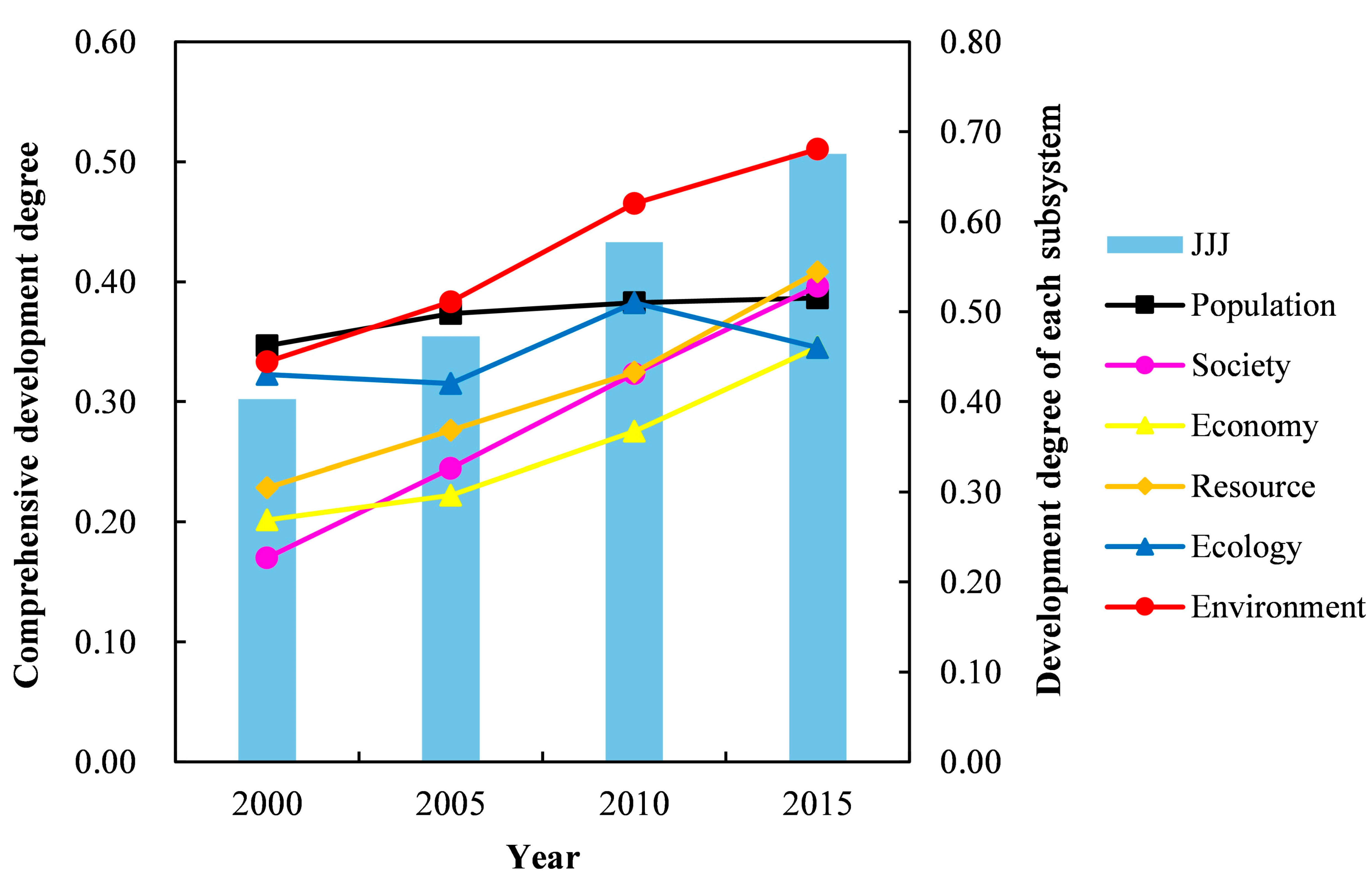
3.2. The Changing Trend of the Whole JJJ and Each Subsystem’s DI

3.2.1. The Changing Trend of DI at the City Scale

Figure 2 showed the changing trend of DI at the city scale. The percent value above the bar diagram was the average annual growth rate of each city’s DI. ZJK (2.44%) and CD (1.33%) were the top two cities in terms of the average annual growth rate of the population subsystem (Figure 2a), whereas TJ was the only city with a negative rate of change. BJ had the highest average DI value (0.70), followed by TJ (0.63). Regarding the society subsystem, BJ had the highest DI value, especially during 2000–2005, with a sharp increase from 0.58 to 0.86, while HS had the lowest DI value with an average value of 0.22. As for the average annual growth rate, CZ had the highest rate (15.59%), while BJ had the lowest one (4.23%), although all cities had been experiencing a continuous increase in DI values. As for the economy subsystem, BJ and TJ were the top two cities in terms of DI value and annual average growth rate (8.11% and 8.02%), while ZJK and QHD were in the lowest position, with the rate of 1.46% and 1.60%, respectively. Except for ZJK and CD, all the left cities showed a continuously increasing economy subsystem trend.

Regarding the resource subsystem, CZ had the highest average DI value (0.60), while CD had the lowest (0.18). Its annual average growth rate was highest in XT (14.51%). Regarding the ecology subsystem, all the left cities except for ZJK showed a fluctuating DI trend; Considering the average value of DI, CD had the highest value (0.61), while XT had the lowest one (0.33). Besides, seven cities had a positive annual average rate of change, especially ZJK, that showed the highest annual average growth rate (2.28%). As for the environment subsystem, BJ had the highest DI value in 2015 (0.90), while HS had the lowest one (0.61), whereas its annual average growth rate was highest in CD (8.25%) and lowest in QHD (1.31%). Generally, BJ achieved the highest average DI value in population, society, economy, and environment, which corresponds to its administrative status; Although CD had the lowest average DI value in resources, it exhibited the highest DI value in ecology, owing to its high vegetation cover.

3.2.2. The Changing Trend of DI at the Urban Agglomeration Scale

Figure 3 displayed the changing trend of DI at the urban agglomeration scale. The comprehensive DI value of JJJ showed a continuous increase from 0.30 (2000) to 0.51 (2015), with an annual average growth rate of 4.51%. For each subsystem, the annual average growth rates were the following: society (8.87%), resource (5.23%), economy (4.75%), environment (3.54%), population (0.77%), and ecology (0.47%). By the end of 2015, the environment subsystem had the highest DI value (0.68), followed by resource (0.54), society (0.53), population (0.52), economy (0.46), and ecology (0.46). DI values were divided into five grades, which were poor (0–0.2), fair (0.2–0.4), moderate (0.4–0.6), good (0.6–0.8), and excellent (0.8–1.0). To this end, the DI value grade improved from “fair” to “moderate.” The grades of population, society, economy, resource, and ecology were found to be “moderate,” and that of the environment was “good” in 2015.

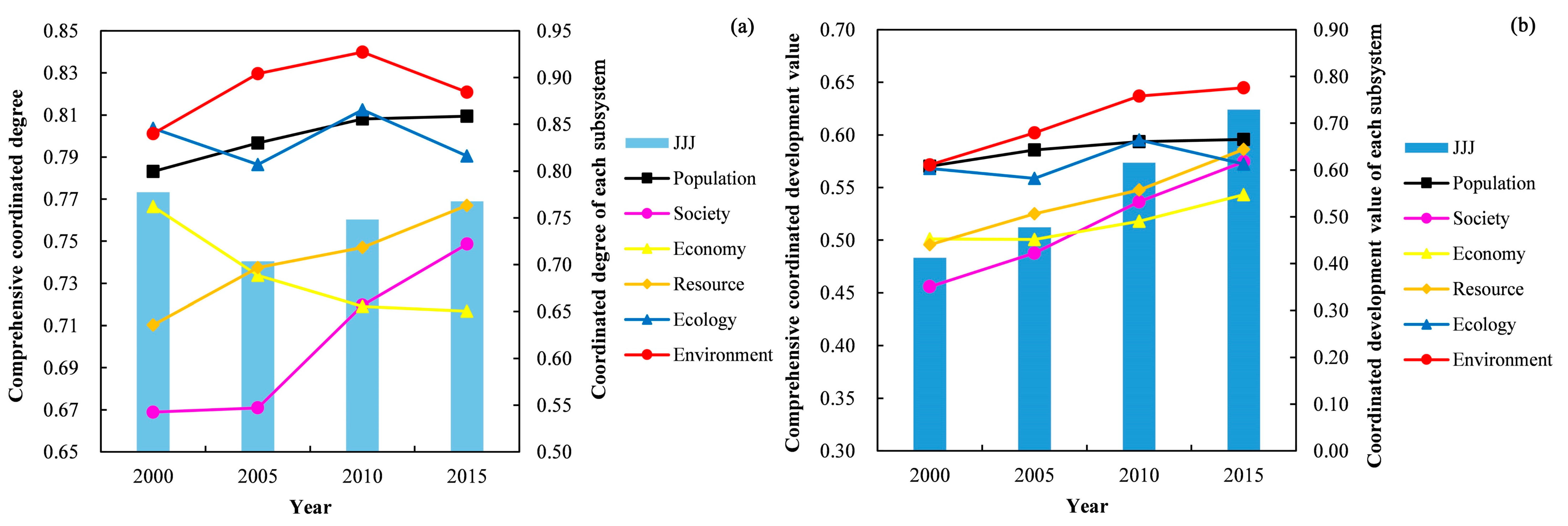
3.3. The Changing Trend of the Whole JJJ and Each Subsystem’s CI Value

Table 6. The coordinated index (CI) value of the whole Jing-Jin-Ji (JJJ) and each subsystem.

Subsystem	2000	2005	2010	2015
Population	0.7996	0.8300	0.8557	0.8588
Society	0.5425	0.5471	0.6566	0.7219
Economy	0.7621	0.6884	0.6554	0.6505
Resource	0.6356	0.6968	0.7184	0.7632
Ecology	0.8457	0.8069	0.8654	0.8162
Environment	0.8401	0.9042	0.9272	0.8843
JJJ	0.7733	0.7404	0.7603	0.7690

shows the whole JJJ and each subsystem’s CI value. Figure 4a illustrates the changing trend of CI at the urban agglomeration scale. Based on Table 6 and Figure 4, the comprehensive CI of JJJ had a “V” shape. The CI value decreased by −1.74% from 2000 to 2015, indicating the wider gap of comprehensive DI value among cities. Among the six subsystems, population, society, resource, and environment exhibited an increasing trend, while economy and ecology decreased. Their annual average growth rates were the following: society (2.21%), resource (1.34%), population (0.49%), environment (0.35%), ecology (−0.23%), and economy (−0.98%). In general, the CI value of the society subsystem increased significantly from 0.5425 (2000) to 0.7219 (2015), indicating that the gap between cities had been gradually narrowed. However, the CI value of the economy subsystem decreased from 0.7621 (2000) to 0.6505 (2015), indicating that the gap between cities had gradually widened. As with DI, we also divided CI into five grades, equally. The comprehensive CI grade of JJJ was found to be “good” during the study period. The grade of the population and society subsystems improved from “good” to “excellent” and “moderate” to “good,” respectively. The grade of the resource subsystem was not changed (“good” all the time). Furthermore, the grade of both the ecology and environment subsystems was “excellent” during 2000–2015. Although the CI value decreased continuously, the economy subsystem’s grade was “good” during the study period.

3.4. The Changing Trend of the Whole JJJ and Each Subsystem’s CDI

Table 7. The coordinated development index (CDI) value of the whole JJJ and each subsystem.

Subsystem	2000	2005	2010	2015
Population	0.6078	0.6427	0.6607	0.6653
Society	0.3507	0.4224	0.5321	0.6175
Economy	0.4529	0.4516	0.4905	0.5475
Resource	0.4402	0.5065	0.5575	0.6444
Ecology	0.6030	0.5822	0.6643	0.6127
Environment	0.6110	0.6798	0.7584	0.7757
JJJ	0.4834	0.5123	0.5737	0.6242

displays the CDI value of the whole JJJ and each subsystem. Figure 4b shows the changing trend of CDI at the urban agglomeration. Based on Table 7 and Figure 4b, we found that the comprehensive CDI value of JJJ displayed a continuously increasing trend, from 0.4834 in 2000 to 0.6242 in 2015. The annual average growth rate was 1.94%. The six subsystems’ CDI values had a positive annual average change rate; the order was society (5.07%) > resource (3.09%) > environment (1.80%) > ecology (1.39%) > population (0.63%) > ecology (0.11%). At the end of 2015, the order of each subsystem’s CDI value was environment (0.7757) > population (0.6653) > resource (0.6444) > society (0.6175) > ecology (0.6127) > economy (0.5475). As with CI and DI, we divided CDI into five grades, equally. Regarding the comprehensive CDI value of JJJ, the grade had improved from “moderate” in 2000 to “good” in 2015. As for the six subsystems, the grade of population was “good” during 2000–2015; society’s grade had improved from “fair” to “good”; economy’s grade was “moderate” all the time; resource’s grade had improved from “moderate” to “good”; ecology’s grade had firstly decreased from “good” to “moderate”, then improved to “good”. In general, combined with CI and DI, we found that the DI and CI value of the economy subsystem displayed a continuously increasing and decreasing trend, respectively; however, the CDI value showed a continuously increasing one, indicating that the gap of all cities’ DI growth rate had widened.

4. Discussion

4.1. Weight Assignment with Existing Studies

In our study, each subsystem’s weight was assigned by combining AHP and EM. We found that the economy subsystem had the highest weight, followed by society, resource, population, ecology, and environment. The economy was one of the most critical subsystems. Previous studies had paid much attention to building economic subsystems. Li and Yi treated the economy as one of the necessary subsystems [3]; Liu et al. constructed an indicator system from the aspects of the economy, society, and environment, with the order of their weight being economy > society > environment [36], which was consistent with our result. Fang et al. studied the green development under the population-resource-environment-development-satisfaction perspective and found that resource had a higher weight than the population subsystem [43]. Besides, several studies assigned the same weight to different subsystems. For instance, Wang et al. analyzed the energy, economy, and environment subsystems by giving the same weight to each of them [34]; Guan et al. also gave the same weight to the urban economy-resource-environment system [28]. However, we thought that different subsystems should have different weights. Former studies thought that the coordinated development should focus on the synchronous development of different subsystems; hence, they gave the same weight to different subsystems. However, based on our definition, we focused on improving the DI of different subsystems and narrowing the DI gap between cities. We believe that the improved DI of different subsystems is ideal for seeking a synchronous development of different subsystems. Since the implementation of the reform and opening-up policy in China, the government puts much emphasis on the economy subsystem. Thus, based on our findings, assigning different weights to different subsystems would be more appropriate.

4.2. Analysis of DI, CI, and CDI and Their Implications

Based on the DI value at the city level, TJ’s population DI showed a negative annual average growth rate (−0.37%) due to its low population quantity and population score, from a value of 0.52 in 2000 to 0.26 in 2015. However, although TJ showed a decreasing trend, it had been ranked second all the time. As one of China’s municipalities, TJ was the Bohai Sea area’s economic center according to the Master Plan of Tianjin (2005–2020). Regarding the society subsystem, the DI value of BJ had sharply increased from 0.58 in 2000 to 0.86 in 2005, mainly because of the sharp increase of the indicator C₅. During 2000–2005, the original value of C₅ had increased from 25.46 (users) to 94.92 (users). Regarding the economy subsystem, the rankings of LF had improved from eleventh (2000) to fifth (2015). Since the Beijing-Tianjin-Hebei Collaborative Development Strategy promotion in 2014, LF has played an increasingly important role in connecting BJ and TJ. Regarding the resource subsystem, in 2015, CZ had the highest DI value owing to the high score of C₁₇; the original value was 1.14 (tons), indicating that CZ had a high utilization efficiency of water resources. CD had the lowest DI value in 2015 because of its low water, energy, and industrial solid waste utilization efficiency. For BJ, its ranking improved from fifth in 2000 to third in 2015 due to its high energy utilization efficiency; however, we found that its water utilization efficiency was very low in 2015 (0.14), and needed to increase in the future. Zhu et al. also reported that BJ’s resource utilization’s overall level was relatively insufficient [47]. Regarding the ecology subsystem, CD had the highest DI value all the time, which had a good relationship with its high vegetation cover. Based on the statistical data from Chengde Forestry and Grassland Bureau, CD had approximately 2.34 million hectares of forest land, accounting for 32% of the total JJJ; Besides, in 2020, the forest cover rate of CD was 59.41%, which was higher than the national level by 36%; the grassland comprehensive vegetation coverage rate was 73.60%. The DI value of ZJK displayed a continuously increasing trend, owing to a series of projects implemented by the government, such as “Returning Farmland to Forest (grass) Project”, “Three-North Shelter Forest Program”, “Beijing-Hebei Ecological Water Resources Protection Forest Project”, etc. To further understand the ecological change situation, based on the normalized ecological time difference index (NETDI) in our previous work [25], all cities’ average NETDI values were calculated based on Equation (21).

$$NETDI=\frac{E{Q}_{T_{end}}-E{Q}_{T_{start}}}{E{Q}_{T_{end}}+E{Q}_{T_{start}}}$$

(21)

where EQ_Tstart and EQ_Tend denote the ecological quality in 2001 and 2015; NETDI ranges from −1 to 1—the higher the value, the higher the improvement of ecological quality, and vice versa.

Table 8. The average normalized ecological time difference index (NETDI) value of each city.

City	NETDI	City	NETDI
BJ	0.0252	BD	0.0438
TJ	−0.0443	ZJK	0.1633
SJZ	−0.0025	CD	0.0418
TS	−0.0275	CZ	0.0450
QHD	0.0160	LF	−0.0029
HD	−0.0962	HS	−0.0511
XT	−0.0339

shows the average NETDI value of each city. It could be found that BJ, QHD, BD, ZJK, CD, and CZ had a positive value, indicating that these cities’ ecological quality had improved. For BJ, similar results were also reported in the Beijing Municipal Ecological Remote Sensing Annual Report (2018). For ZJK, as we have mentioned above, series projects had been mainly implemented in this city. However, TJ, SJZ, TS, HD, XT, LF, and HS had a negative value, indicating that these cities’ ecological quality had slightly declined. Wang et al. found similar results: the ecological quality of CD, BJ, QHD, and BD was higher than JJJ’s average level, while LF, TJ, and CZ were lower than JJJ’s average level [52].

Regarding the environment subsystem, all cities’ DI values had increased during 2000–2015 due to the sharp improvement of the environmental governance level, which had increased from 0.56 to 0.96. The population subsystem’s growth rate gradually slowed down at the urban agglomeration scale due to its low development value in population quantity. Zhu et al. calculated all cities’ population carrying capacity and found that all JJJ cities need population regulation (such as population structure improvement and optimization of population spatial distribution pattern) [47].

Based on the CI value at the urban agglomeration scale, population, ecology, and environment had a relatively high CI value, indicating that their DI gap between cities was not high. Regarding the society subsystem, the CI value had increased a lot since 2005, indicating that the basic public service level and infrastructure construction level had improved. To achieve an equalization of basic public services, the Chinese central government decided to steadily improve public services equalization during the 13th 5-Year Plan period (2016–2020) [53]. Regarding the economy subsystem, its CI value displayed a continuously decreasing trend, although all cities’ economy DI had improved. However, the economic gap between cities had widened. Zhao et al. also found that the economic disparity in JJJ had widened [54].

Table 9. The CI value of all indicators during 2000–2015.

Indicator	CI				Indicator	CI
	2000	2005	2010	2015		2000	2005	2010	2015
C1	0.5389	0.5510	0.5091	0.4544	C14	0.4016	0.3185	0.3098	0.2880
C2	0.8567	0.8741	0.8760	0.8502	C15	0.5682	0.5545	0.5665	0.5725
C3	0.5844	0.7404	0.8015	0.8613	C16	0.7829	0.7343	0.7346	0.7737
C4	0.9131	0.9058	0.9106	0.8786	C17	0.4684	0.4729	0.4830	0.4761
C5	0.5413	0.5929	0.7980	0.8739	C18	0.5030	0.6968	0.6198	0.6584
C6	0.4885	0.4647	0.4873	0.5157	C19	0.6503	0.6727	0.6952	0.7625
C7	0.5964	0.6354	0.6166	0.6306	C20	0.8457	0.8069	0.8654	0.8162
C8	0.6808	0.6882	0.7807	0.8435	C21	0.7366	0.7035	0.6983	0.7253
C9	0.6814	0.6890	0.8475	0.8993	C22	0.5482	0.6659	0.5312	0.5392
C10	0.2682	0.2510	0.4739	0.5010	C23	0.5055	0.4829	0.4358	0.2506
C11	0.2647	0.3787	0.4497	0.4390	C24	0.7072	0.8524	0.9451	0.9672
C12	0.3432	0.3733	0.4051	0.4651	C25	0.6902	0.7898	0.9517	0.9353
C13	0.4047	0.4260	0.3744	0.5156

shows the CI value of all indicators.

Based on Table 9, it could be found that the CI values of nine indicators (C₁, C₂, C₄, C₁₄, C₁₆, C₂₀, C₂₁, C₂₂, and C₂₃) exhibited a decreasing trend during 2000–2015. C₂₃ had the lowest rate (−3.36%), indicating that the gap of this indicator between cities had widened from the aspects of the annual average growth rate. Furthermore, C₂₁, C₂₂, and C₂₃ all belonged to the environmental pollution attribute. Regarding the indicators with a positive rate, C₁₀ had the highest value (5.79%). Besides, all society subsystem indicators displayed a positive change rate, indicating that the gap of society development level between cities had narrowed. By the end of 2015, the CI value of C₁, C₁₁, C₁₂, C₁₄, C₁₇, and C₂₃ was lower than 0.5. Based on the CDI value at the urban agglomeration scale, the whole JJJ and six subsystems all displayed an increasing trend, indicating that the coordinated development level had improved, which was similar to Zhu’s findings [47]. However, based on

Table 10. The CDI value of all indicators during 2000–2015.

Indicator	CDI				Indicator	CDI
	2000	2005	2010	2015		2000	2005	2010	2015
C1	0.3779	0.3715	0.3104	0.2591	C14	0.1128	0.1490	0.2133	0.2596
C2	0.7774	0.8105	0.8236	0.8026	C15	0.2296	0.3104	0.4330	0.5218
C3	0.5233	0.6720	0.7420	0.8173	C16	0.6105	0.5879	0.6031	0.6622
C4	0.6983	0.7135	0.7457	0.7450	C17	0.1607	0.2358	0.3279	0.4013
C5	0.2253	0.4678	0.7344	0.8716	C18	0.3436	0.4214	0.4368	0.5504
C6	0.3438	0.3905	0.4210	0.4650	C19	0.6374	0.7019	0.7304	0.7973
C7	0.3549	0.4568	0.4659	0.5473	C20	0.6030	0.5822	0.6643	0.6127
C8	0.6140	0.5828	0.6971	0.7992	C21	0.6137	0.5939	0.5886	0.6599
C9	0.5447	0.5515	0.7155	0.8079	C22	0.4537	0.4161	0.4116	0.4833
C10	0.1915	0.2214	0.3463	0.3754	C23	0.2222	0.1957	0.2289	0.2140
C11	0.2087	0.3405	0.3974	0.4026	C24	0.7303	0.8584	0.9614	0.9748
C12	0.3130	0.3394	0.3732	0.4215	C25	0.5032	0.6994	0.9149	0.9319
C13	0.1436	0.2232	0.2847	0.3909

, it could be found that ten indicators’ CDI (C₁, C₆, C₁₀, C₁₁, C₁₂, C₁₃, C₁₄, C₁₇, C₂₂, and C₂₃) was lower than 0.5 at all times, and these indicators mainly belonged to the basic public service and environmental pollution aspects, indicating that the government still needs to work hard to improve both aspects.

4.3. Limitations and Further Study

The CDI of the JJJ urban agglomeration during 2000–2015 has been investigated. However, this study still has some limitations. Firstly, the indicator system is not imperfect. Although we have carefully selected representative indicators to evaluate the CDI, we had to ignore some aspects; secondly, as we have discussed above, the six subsystems’ weight was determined by the combination of AHP and EM. However, weight assignment involves numerous aspects; in the future, more studies could be done to combine and compare newly developed weighting methods to assign the different subsystems a more appropriate weight. Finally, in our study, we only calculated the CDI of JJJ in the past years; although these results could provide some suggestions for relevant policymakers, we still need to predict the future state with some models, like the system dynamic model.

5. Conclusions

This study used statistical data and non-statistical data to evaluate JJJ’s DI, CI, and CDI at the city and urban agglomeration scales during 2000–2015. The main conclusions were as follows: (1) The economy subsystem had the highest weight; (2) At the city scale, BJ had the highest comprehensive DI value, followed by TJ; at the urban agglomeration scale, the comprehensive DI value of JJJ had increased from 0.30 in 2000 to 0.51 in 2015, with the improvement of grade from “fair” to “moderate”; (3) The comprehensive CI value of JJJ displayed a “V” shape, with an annual average growth rate of −0.04%; among the different subsystems, the CI value of the economy subsystem showed a continuous decrease from 0.7621 (2000) to 0.6505 (2015); (4) The comprehensive CDI value of JJJ increased from 0.39 to 0.59, with the change of its grade from “fair” to “moderate” during the study period.

References

1. Wen, Q.; Zhang, Z.; Shi, L.; Zhao, X.; Liu, F.; Xu, J.; Yi, L.; Liu, B.; Wang, X.; Zuo, L.; et al. Extraction of basic trends of urban expansion in China over past 40 years from satellite images. Chin. Geogr. Sci. 2016, 26, 129–142. [Google Scholar] [CrossRef] [Green Version]
2. Shi, L.; Taubenböck, H.; Zhang, Z.; Liu, F.; Wurm, M. Urbanization in China from the end of 1980s until 2010—Spatial dynamics and patterns of growth using EO-data. Int. J. Digit. Earth 2019, 12, 78–94. [Google Scholar] [CrossRef]
3. Li, W.; Yi, P. Assessment of city sustainability—Coupling coordinated development among economy, society and environment. J. Clean. Prod. 2020, 256, 120453. [Google Scholar] [CrossRef]
4. Xie, M.; Wang, J.; Chen, K. Coordinated development analysis of the “Resources-environment-ecology-economy-society” complex system in China. Sustainability 2016, 8, 582. [Google Scholar] [CrossRef] [Green Version]
5. Qin, C.; Zheng, Y.; Zhang, H. A study on the tendencies and features of the coordinated development of regional economy in China. Econ. Geogr. 2013, 33, 9–14. (In Chinese) [Google Scholar] [CrossRef]
6. Bolcárová, P.; Kološta, S. Assessment of sustainable development in the EU 27 using aggregated SD index. Ecol. Indic. 2015, 48, 699–705. [Google Scholar] [CrossRef]
7. Li, Q.; Dang, Y.; Wang, Z. Analysis of the regional coordination development systems based on GRA and GM(1,N). J. Grey Syst. 2012, 24, 35–100. [Google Scholar]
8. Liu, H.; Liu, Y.; Wang, H.; Yang, J.; Zhou, X. Research on the coordinated development of greenization and urbanization based on system dynamics and data envelopment analysis—A case study of Tianjin. J. Clean. Prod. 2019, 214, 195–208. [Google Scholar] [CrossRef]
9. Fang, C.; Cui, X.; Li, G. Modeling regional sustainable development scenarios using the urbanization and eco-environment coupler: Case study of Beijing-Tianjin-Hebei urban agglomeration, China. Sci. Total Environ. 2019, 59, 102208. [Google Scholar] [CrossRef] [PubMed]
10. Zhang, Q.; Wang, L.; Wu, F.; Yuan, L.; Zhao, L. Quantitative evaluation for coupling coordinated development between ecosystem and economic system-case study of Chinese loess plateau. J. Urban Plan. Dev. 2012, 138, 328–334. [Google Scholar] [CrossRef]
11. Sun, Q.; Zhang, X.; Zhang, H.; Niu, H. Coordinated development of a coupled social economy and resource environment system: A case study in Henan Province, China. Environ. Dev. Sustain. 2018, 20, 1385–1404. [Google Scholar] [CrossRef]
12. Lin, X.; Lu, C.; Song, K.; Su, Y.; Lei, Y.; Zhong, L.; Gao, Y. Analysis of Coupling Coordination Variance between Urbanization Quality and Eco-Environment Pressure: A Case Study of the West Taiwan Strait Urban Agglomeration, China. Sustainability 2020, 12, 2643. [Google Scholar] [CrossRef] [Green Version]
13. Li, W.; Yi, P.; Zhang, D.; Zhou, Y. Assessment of coordinated development between social economy and ecological environment: Case study of resource-based cities in Northeastern China. Sustain. Cities Soc. 2020, 59, 102208. [Google Scholar] [CrossRef]
14. Fan, Y.; Fang, C.; Zhang, Q. Coupling coordinated development between social economy and ecological environment in Chinese provincial capital cities-assessment and policy implications. J. Clean. Prod. 2019, 229, 289–298. [Google Scholar] [CrossRef]
15. Zameer, H.; Yasmeen, H.; Wang, R.; Tao, J.; Malik, M. An empirical investigation of the coordinated development of natural resources, financial development and ecological efficiency in China. Resour. Policy 2020, 65, 101580. [Google Scholar] [CrossRef]
16. Zhang, P.; Yuan, H.; Tian, X. Sustainable development in China: Trends, patterns, and determinants of the “Five Modernizations” in Chinese cities. J. Clean. Prod. 2019, 214, 685–695. [Google Scholar] [CrossRef]
17. Ma, L.; Cheng, W.; Qi, J. Coordinated evaluation and development model of oasis urbanization from the perspective of new urbanization: A case study in Shandan County of Heixi Corridor, China. Sustain. Cities Soc. 2018, 39, 78–92. [Google Scholar] [CrossRef]
18. Ariken, M.; Zhang, F.; Liu, K.; Fang, C.; Kung, H. Coupling coordination analysis of urbanization and eco-environment in Yanqi Basin based on multi-source remote sensing data. Ecol. Indic. 2020, 114, 106331. [Google Scholar] [CrossRef]
19. Tian, Y.; Zhou, D.; Jiang, G. Conflict or coordination? Multiscale assessment of the spatio-temporal coupling relationship between urbanization and ecosystem services: The case of the Jingjinji region, China. Ecol. Indic. 2020, 117, 106543. [Google Scholar] [CrossRef]
20. Yang, C.; Zeng, W.; Yang, X. Coupling coordination evaluation and sustainable development pattern of geo-ecological environment and urbanization in Chongqing municipality, China. Sustain. Cities Soc. 2020, 61, 102271. [Google Scholar] [CrossRef]
21. Shao, Z.; Ding, L.; Li, D.; Altan, O.; Huq, M.; Li, C. Exploring the Relationship between Urbanization and Ecological Environment Using Remote Sensing Images and Statistical Data: A Case Study in the Yangtze River Delta, China. Sustainability 2020, 12, 5620. [Google Scholar] [CrossRef]
22. Xu, H.; Wang, Y.; Guan, H.; Shi, T.; Hu, X. Detecting ecological changes with a remote sensing based ecological index (RSEI) produced time series and change vector analysis. Remote Sens. 2019, 11, 2345. [Google Scholar] [CrossRef] [Green Version]
23. Xu, H. A remote sensing urban ecological index and its application. Acta Ecol. Sin. 2013, 33, 7853–7862. (In Chinese) [Google Scholar] [CrossRef]
24. Ji, J.; Wang, S.; Zhou, Y.; Liu, W.; Wang, L. Spatiotemporal Change and Landscape Pattern Variation of Eco-Environmental Quality in Jing-Jin-Ji Urban Agglomeration From 2001 to 2015. IEEE Access 2020, 8, 125534–125548. [Google Scholar] [CrossRef]
25. Ji, J.; Wang, S.; Zhou, Y.; Liu, W.; Wang, L. Studying the Eco-Environmental Quality Variations of Jing-Jin-Ji Urban Agglomeration and Its Driving Factors in Different Ecosystem Service Regions from 2001 to 2015. IEEE Access 2020, 8, 154940–154952. [Google Scholar] [CrossRef]
26. Sun, C.; Chen, L.; Tian, Y. Study on the urban state carrying capacity for unbalanced sustainable development regions: Evidence from the Yangtze River Economic Belt. Ecol. Indic. 2018, 89, 150–158. [Google Scholar] [CrossRef]
27. Meijering, J.; Tobi, H.; Kern, K. Defining and measuring urban sustainability in Europe: A Delphi study on identifying its most relevant components. Ecol. Indic. 2018, 90, 38–46. [Google Scholar] [CrossRef]
28. Guan, D.; Gao, W.; Su, W.; Li, H.; Hokao, K. Modeling and dynamic assessment of urban economy-resource-environment system with a coupled system dynamics—Geographic information system model. Ecol. Indic. 2011, 11, 1333–1344. [Google Scholar] [CrossRef]
29. Fan, W.; Wang, H.; Liu, Y.; Liu, H. Spatio-temporal variation of the coupling relationship between urbanization and air quality: A case study of Shandong Province. J. Clean. Prod. 2020, 272, 122812. [Google Scholar] [CrossRef]
30. Gong, Q.; Chen, M.; Zhao, X.; Ji, Z. Sustainable urban development system measurement based on dissipative structure theory, the grey entropy method and coupling theory: A case study in Chengdu, China. Sustainability 2019, 11, 293. [Google Scholar] [CrossRef] [Green Version]
31. Cui, X.; Fang, C.; Liu, H.; Liu, X. Assessing sustainability of urbanization by a coordinated development index for an Urbanization-Resources-Environment complex system: A case study of Jing-Jin-Ji region, China. Ecol. Indic. 2019, 96, 383–391. [Google Scholar] [CrossRef]
32. Sun, Y.; Cui, Y. Evaluating the coordinated development of economic, social and environmental benefits of urban public transportation infrastructure: Case study of four Chinese autonomous municipalities. Transport Policy 2018, 66, 116–126. [Google Scholar] [CrossRef]
33. Lu, C.; Yang, J.; Li, H.; Jin, S.; Pang, M.; Lu, C. Research on the spatial-temporal synthetic measurement of the coordinated development of population-economy-society-resource-environment (PESRE) systems in China based on geographic information systems (GIS). Sustainability 2019, 11, 2877. [Google Scholar] [CrossRef] [Green Version]
34. Wang, Q.; Yuan, X.; Cheng, X.; Mu, R.; Zuo, J. Coordinated development of energy, economy and environment subsystems—A case study. Ecol. Indic. 2014, 46, 514–523. [Google Scholar] [CrossRef]
35. Yang, Y.; Hu, N. The spatial and temporal evolution of coordinated ecological and socioeconomic development in the provinces along the Silk Road Economic Belt in China. Sustain. Cities Soc. 2019, 47, 101466. [Google Scholar] [CrossRef]
36. Liu, Y.; Xu, J.; Luo, H. An integrated approach to modelling the economy-society-ecology system in urbanization process. Sustainability 2014, 6, 1946–1972. [Google Scholar] [CrossRef] [Green Version]
37. Duan, Y.; Mu, H.; Li, N.; Li, L.; Xue, Z. Research on comprehensive evaluation of low carbon economy development level based on AHP-entropy method: A case study of Dalian. Energy Procedia 2016, 104, 468–474. [Google Scholar] [CrossRef]
38. Cheng, X.; Long, R.; Chen, H.; Li, Q. Coupling coordination degree and spatial dynamic evolution of a regional green competitiveness system—A case study from China. Ecol. Indic. 2019, 104, 489–500. [Google Scholar] [CrossRef]
39. Li, Y.; Li, Y.; Zhou, Y.; Shi, Y.; Zhu, X. Investigation of a coupling model of coordination between urbanization and the environment. J. Environ. Manag. 2012, 98, 127–133. [Google Scholar] [CrossRef]
40. He, J.; Wang, S.; Liu, Y.; Ma, H.; Liu, Q. Examining the relationship between urbanization and the eco-environment using a coupling analysis: Case study of Shanghai, China. Ecol. Indic. 2017, 77, 185–193. [Google Scholar] [CrossRef]
41. Xu, M.; Hu, W. A research on coordination between economy, society and environment in China: A case study of Jiangsu. J. Clean. Prod. 2020, 258, 120641. [Google Scholar] [CrossRef]
42. Cui, D.; Chen, X.; Xue, Y.; Li, R.; Zeng, W. An integrated approach to investigate the relationship of coupling coordination between social economy and water environment on urban scale—A case study of Kunming. J. Environ. Manage. 2019, 234, 189–199. [Google Scholar] [CrossRef]
43. Fang, C.; Wang, Q.; Tian, L. Green development of Yangtze River Delta in China under Population-Resources-Environment-Development-Satisfaction perspective. Sci. Total Environ. 2020, 727, 138710. [Google Scholar] [CrossRef]
44. Xue, W.; Zhang, J.; Zhong, C.; Li, X.; Wei, J. Spatiotemporal PM2.5 variations and its response to the industrial structure from 2000 to 2018 in the Beijing-Tianjin-Hebei region. J. Clean. Prod. 2021, 279, 123742. [Google Scholar] [CrossRef]
45. Wan, Z. New refinements and validation of the collection-6 MODIS land-surface temperature/emissivity product. Remote Sen. Environ. 2014, 140, 36–45. [Google Scholar] [CrossRef]
46. Li, Y.; Sun, Z. The development of western new-type urbanization level evaluation based on entropy method. On Econ. Probl. 2015, 3, 115–119. (In Chinese) [Google Scholar] [CrossRef]
47. Zhu, H.; Ye, T.; Zhang, G. Annual Report on Beijing-Tianjin-Hebei Metropolitan Region Development Report (2017); Beijing Social Sciences Academic Press: Beijing, China, 2017; pp. 273–295. (In Chinese) [Google Scholar]
48. Hebei Province Issued the “Hebei Population Development Plan (2018–2035)”. Available online: http://hebei.hebnews.cn/2018-10/06/content_7053479.htm (accessed on 6 October 2018).
49. Yao, S. Study on the Comprehensive Evaluation of Population Development in Shandong Province. Master’s Thesis, University of Chinese Academy of Sciences, Beijing, China, April 2015. [Google Scholar]
50. Guiding Principles for the Establishment of Medical Institutions (2016–2020). Available online: http://www.gov.cn/xinwen/2016-08/16/content_5099736.htm (accessed on 16 August 2016).
51. Ambient Air Quality Standards. Available online: http://www.mee.gov.cn/ywgz/fgbz/bz/bzwb/dqhjbh/dqhjzlbz/201203/t20120302_224165.htm (accessed on 1 January 2016).
52. Wang, J.; Zhou, W.; Xu, K.; Yan, J.; Li, W.; Han, L. Quantitative assessment of ecological quality in Beijing-Tianjin-Hebei urban megaregion. Chin. J. Appl. Ecol. 2017, 28, 2667–2676. (In Chinese) [Google Scholar] [CrossRef]
53. Li, Z.; He, S.; Su, S.; Li, G.; Chen, F. Public services equalization in urbanizing China: Indicators, spatiotemporal dynamics and implications on regional economic disparities. Soc. Indic. Res. 2020, 152, 1–65. [Google Scholar] [CrossRef]
54. Zhao, X.; Zhou, W.; Lu, J. A study on spatial difference of regional economic of Beijing, Tianjin and Hebei. J. Ind. Technol. Econ. 2015, 34, 46–51. (In Chinese) [Google Scholar] [CrossRef]
Figure 1. Location of the study area.
Sustainability 13 04075 g001
Figure 2. The changing trend of the development degree value (DI) at the city scale. (a) The DI of the population subsystem; (b) The DI of the society subsystem; (c) The DI of the economy subsystem; (d) The DI of the resource subsystem; (e) The DI of the ecology subsystem; (f) The DI of the environment subsystem.
Sustainability 13 04075 g002
Figure 3. The changing trend of DI at the urban agglomeration scale.
Sustainability 13 04075 g003
Figure 4. The changing trend of CI and CDI at urban agglomeration scale. (a) The changing trend of CI; (b) The changing trend of CDI.
Sustainability 13 04075 g004