TOPOI RESOURCES: Quantification and Assessment of Global Warming Potential and Land-Uptake of Residential Buildings in Settlement Types along the Urban–Rural Gradient—Opportunities for Sustainable Development

Mühlbach, Ann-Kristin; Mumm, Olaf; Zeringue, Ryan; Redbergs, Oskars; Endres, Elisabeth; Carlow, Vanessa Miriam

doi:10.3390/su13084099

Open AccessArticle

TOPOI RESOURCES: Quantification and Assessment of Global Warming Potential and Land-Uptake of Residential Buildings in Settlement Types along the Urban–Rural Gradient—Opportunities for Sustainable Development

¹

TU Braunschweig, Institute for Building Services and Energy Design (IGS), Mühlenpfordtstr. 23, 38106 Braunschweig, Germany

²

TU Braunschweig, Institute for Sustainable Urbanism (ISU), Pockelsstr. 3, 38106 Braunschweig, Germany

^*

Authors to whom correspondence should be addressed.

Sustainability 2021, 13(8), 4099; https://0-doi-org.brum.beds.ac.uk/10.3390/su13084099

Submission received: 26 February 2021 / Revised: 26 March 2021 / Accepted: 29 March 2021 / Published: 7 April 2021

(This article belongs to the Special Issue Sustainability Assessment of Architecture, Construction, Refurbishment and Restoration)

Download

Browse Figures

Versions Notes

Abstract

:

The METAPOLIS as the polycentric network of urban–rural settlement is undergoing constant transformation and urbanization processes. In particular, the associated imbalance of the shrinkage and growth of different settlement types in relative geographical proximity causes negative effects, such as urban sprawl and the divergence of urban–rural lifestyles with their related resource, land and energy consumption. Implicitly related to these developments, national and global sustainable development goals for the building sector lead to the question of how a region can be assessed without detailed research and surveys to identify critical areas with high potential for sustainable development. In this study, the TOPOI method is used. It classifies settlement units and their interconnections along the urban–rural gradient, in order to quantify and assess the land-uptake and global warming potential driven by residential developments. Applying standard planning parameters in combination with key data from a comprehensive life cycle assessment of the residential building stock, a detailed understanding of different settlement types and their associated resource and energy consumption is achieved.

Keywords:

life cycle assessment; LCA; settlement types; CO₂ emissions; GWP; land-uptake; density; urban–rural development; TOPOI; sustainability

1. Introduction

Urban–rural systems can be described as interconnected settlement units linked by networks and flows of people, goods, information and services [1,2]. Usually, they are characterised by high dynamics in transformation processes, which have an impact on individual settlement units as well as on the general settlement patterns [3,4,5]. There are various approaches offering insights into urban–rural relations [4] such as Netzstadt [1], Zwischenstadt [6], or Metacity [7] and newly Metapolis [8]. However, a prevailing lack of sufficiently integrated urban–rural planning strategies [9] often results in increased land consumption for housing and infrastructure and higher resources and energy demands [10]. Significant interrelations between these phenomena and impacts are observed [11,12,13].

This article focuses on the energy and resource consumption of residential developments along the rural–urban gradient. In particular, phenomena of simultaneous settlement growth, including urban sprawl and shrinkage, including vacancies and associated diverging lifestyles, lead to increased land consumption, diverging demand for resources, greater land requirements for housing and high energy consumption. Land-uptake by urban and other artificial land development in the European Union (EU) amounted to 539 km²/year for the years 2012 to 2018 [14].

The main driver of the increasing land-uptake is the expansion of “industrial and commercial sites”, including structures under construction. This accounts for a share of nearly 60% (approx. 1860 km²) [15]. The “urban diffuse residential expansion” is already the second strongest driver of the increasing land consumption with a share of 12% (390 km²) in total. In Germany, the land covered by settlements and transport infrastructure expanded by around 28% from 40,305 to 51,489 km² between 1992 and 2019 [16]. The 4-year average land-uptake for 2015 to 2018 was 56 hectares per day (204.4 km²/year) [17]. The increase in land-uptake, both proportionately and in relation to the number of inhabitants, becomes smaller with increasing settlement density [18,19].

Besides the demand on the finite resource of land, the building sector represents a significant share of the use of abiotic material and energy for construction and operation. Residential buildings make up to 75% of the EU’s building stock, wholesale, retail and office buildings 7%, and industrial buildings 1% [20]. In the EU, approx. 65% (Germany: approx. 73%) of residential buildings were built before 1980 [20,21]. Within the building sector in Germany, residential buildings have a share of 87.5% of the total building stock and are responsible for 64% of the total end-energy consumption of all buildings [22].

The goal of the German federal government to reach a “nearly climate-neutral” building stock by 2050 leads the focus of future sustainability measures to the buildings sector [23]. In 2019, the building sector was responsible for around 14% of the total greenhouse gas (GHG) emissions in Germany. In a holistic view of the GHG emissions caused by buildings, the emissions for the provision of electricity and heat previously assigned to the energy sector, as well as the emissions assigned to the industrial sector for the production of building materials and buildings services, must also be considered. Using this framework, buildings account for approximately 40% of total GHG emissions in Germany [24]. This difference of 25% shows that the cross-sectoral consideration in terms of the entire life cycle of a building is necessary and has a decisive impact on the achievement of climate protection targets. Within the last years, the impact of the energy used for the construction of a building is increasing, due to new energy saving regulations to reduce the energy demands in the operational phase (heating and electricity). The operation of a building still has a larger impact with around 60%; nevertheless, 40% of energy for the construction of a new building is not negligible [25]. As this study is focusing on the existing residential building stock, the share of so-called embodied energy—energy used for raw material mining, storage, transport, construction of building material and disposal—is lower than for a new building. Nevertheless, the calculation of embodied energy shows how much energy has already been used in the past and that demolition with a new substitute building may be a questionable solution for sustainable future developments.

In order to address the challenges of sustainable development, an evaluation of the building stock, its energy and resource consumption in relation to different settlement types and their specific characteristics is required. Studies on building types as sustainable solutions often focus on the individual building but not on settlement units to take a holistic point of view on a regional level. The method presented in this paper draws on a combination of available data on different scales, to describe the existing building stock without the need of detailed surveys. This approach offers to analyse a whole region by using settlement units and building classifications. The evaluation will focus on the building’s footprint in terms of the global warming potential (GWP) on the one hand and land-uptake on the other.

The objectives of this study are as follows: (a) to develop a multi-scale analysis method for quantifying and assessing the land-uptake and CO₂ emissions of the residential building stock at both the regional and settlement unit level; (b) to identify the interrelations between resource and energy consumption and density (population and buildings) for respective settlement types; (c) to identify a derivation of possible approaches for sustainable development in urban–rural regions.

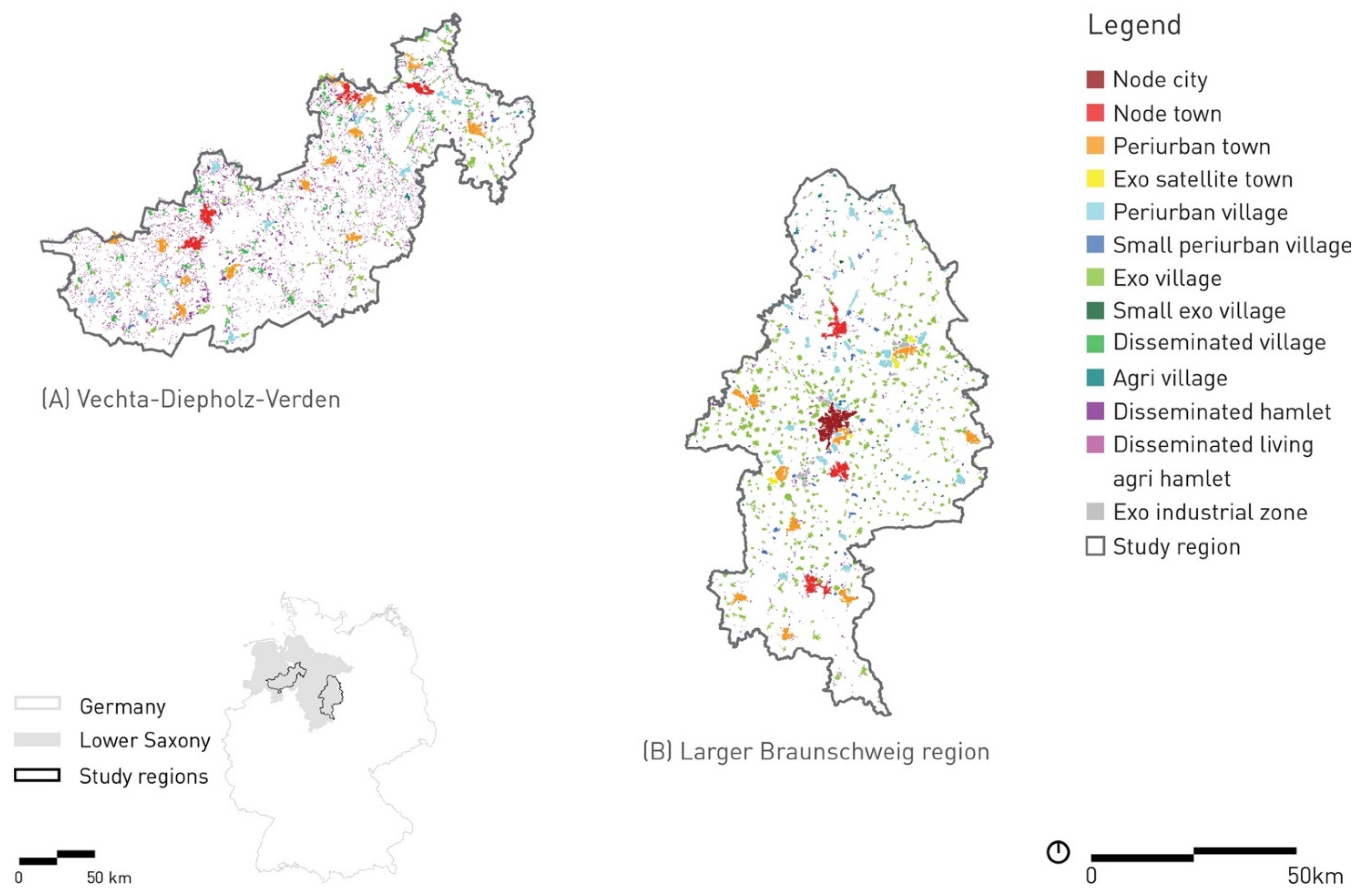
2. The Urban–Rural Settlement System of Lower Saxony

In this research, two regions in Lower Saxony (Germany) are examined: (A) Vechta-Diepholz-Verden, and (B) the larger Braunschweig region (see Figure 1). Simultaneous shrinkage and growth in close geographical proximity are characteristic for the recent and current development of Lower Saxony, with often unsustainable effects, such as a high sealing of land and dense commuting patterns [2,10]. The study region Vechta-Diepholz-Verden is characterised by a large number of evenly distributed, predominantly prosperous medium-sized and small towns in a rural setting. The larger Braunschweig region, meanwhile, includes both prospering cities and shrinking municipalities [3].

To this day, the German spatial planning system is based on the theory of central places [26,27]. It distinguishes between large cities with above 100,000 inhabitants, medium-sized towns between 20,000 and 100,000 inhabitants, small towns with up to 20,000 and villages with less than 5000 inhabitants [26,28]. Settlement types are classified as city (county free), urban county, rural county with densification tendencies or as sparsely populated rural county [29]. In Lower Saxony, only 20% of the population live in large cities (>100,000 Inh.) and 9% in medium-sized towns. With 71%, the majority of the population lives in small towns (<50,000 Inh.), suburban, and rural areas [30]. The two study regions exemplarily reflect the diverse spatial development patterns in Lower Saxony [30,31].

In Germany, around 87.5% of all buildings are residential buildings, which shows the significance of the development of sustainable scenarios for residential buildings [22]. Therefore, this study focuses on the residential building stock. Of all residential buildings in Germany, 78.1% are single- or two-family houses. In Lower Saxony, the share of single- and two-family houses is even higher with 85.1%, and within the study regions their share is 88.1%. The distribution of the building age of existing buildings within the study regions correlates to the distribution in Lower Saxony and the whole of Germany: the majority of the residential buildings were built before 1976 with 62.8% in the study regions (66.6% Lower Saxony, 68.3% Germany). The share of buildings with a higher energy saving standard (built after 1995, see Section 5.3) in the study regions is 19.6%, while it is only 13.9% in Lower Saxony and 12.1% in Germany [32]. This shows that comparatively more buildings have been built in the study regions in recent years than the national average. The following investigations will show the distribution of building types and construction year classes in detail in order to analyse possibilities of a more sustainable future development of the two study regions.

Understanding urbanisation patterns and their relationships along the urban–rural gradient towards a new approach to sustainable development [2,33] requires a comprehensive approach to the analysis and planning of urban regions, encompassing cities and their surrounding areas with multi-faceted interactions, interdependencies, spatial linkages and a fluid transition between urban and rural lifestyles [11,12]. The study utilises the analytical framework of the TOPOI method [2], which describes the urban–rural settlement system in greater detail than the standard planning approach allows. The latter is based on population sizes within administrative boundaries [28] while the TOPOI method enhances the understanding of the built environment by clustering and describing settlement units along similar characteristics of their physical form, function and connectivity based on building footprints (see Table A1 and Table A2) [2]. A settlement unit is understood as a cohesively built group of buildings. This enables a high resolution and comprehensive analysis and interpretation of changes in the physical environment in order to derive recommendations for sustainable transformation.

Applying the TOPOI method, 13 settlement types have been identified for the two study regions (see Figure 1). The TOPOI types include isolated and dispersed units, at the urban fringe or urban cores. Describing the centrality degree of the settlements, the prefixes exo, disseminated, periurban and node are used (see Table A2 and Table A3) [2,31]. The authors expanded the TOPOI method to include energy and resource-related parameters to identify unsustainable and more sustainable development patterns of different settlement types along the urban–rural gradient.

3. Materials

In this study, data-based methods of geospatial analysis are applied, utilizing ArcGIS Pro 2.5.1 [34] using geospatial data from ALKIS (Authoritative Real Estate Cadastre Information System) [35], the Digital Landscape Model (Basis DLM; DLM250) of the Authoritative Topographic-Cartographic Information System (ATKIS) [36,37], and OpenStreetMap [38] as well as life cycle assessment data of residential buildings (see Section 3.1 and Section 3.2) and statistical data from the 2011 German Census ([32]; see Section 3.3).

3.1. Life Cycle Assessment Data—Residential Building Stock

The authors developed a method to quantify the energy demand and resources of the entire residential building stock on a regional scale with a resolution at the settlement unit level. The building stock was classified by building types and construction year classes based on a study by the Institute for Housing and Environment (IWU) [39]. Similar data are not available for other types of buildings, such as industrial or office buildings. Taking this classification into consideration (see Table 1 and Table 2), for each combination a life cycle assessment was conducted. The embodied energy calculation includes the life cycle phase “production” with all environmental impacts of the production of building material, as well as the “maintenance” of buildings during operation, as for example the repair or replacement of damaged building components [40]. The assessment is based on typical structures and building materials for each building type and age [39], using the Ökobaudat (standardized database for ecological evaluations of buildings [41]) and the tool eLCA of the Federal Institute for Research on Buildings, Urban Affairs and Spatial Development [42] for the life cycle assessments. Energy consumption is calculated by average benchmark data for residential buildings, considering the specific building type and age, as well as the energy supply distribution [39,43]. For the building stock, a renovation rate of 1% is considered [22], starting in 1995 after the third thermal insulation ordinance. There is a certain percentage of buildings which are protected for heritage purposes and therefore are excluded from the renovation calculations: this applies to 5% (based on the net floor area) of buildings built between 1949 and 1994, 10% (single-family houses (SFHs)) and 20% (multi-family houses (MFHs)) of buildings built before 1948, based on an estimation of the Institute for Applied Ecology [44]. An assumption for already renovated old buildings (until 1978) of 17.7% for single-family and terraced houses and 21% for multi-family houses and apartment block was included in the calculation, based on Hoier and Erhorn [45]. The embodied energy for building services is not included in the calculations, due to data availability.

3.2. Life Cycle Assessment Data–Streets

In addition to the building stock, the embodied energy of streets within the settlement units is quantified. The classification of OpenStreetMap (OSM) [46] has been used to identify the road types (see Table A5). For each type, a basic layer structure and size has been defined in accordance with the guidelines of the German Road and Transportation Research Association (FGSV) [47,48,49,50]. This was used for the calculation of embodied energy and maintenance for one meter length of each road type, by conducting a life cycle assessment with eLCA [42] and data from Ökobaudat [41]. These results can be combined with the total length of each road type in both study regions, which is available from OSM data [38].

3.3. German Census 2011

The spatial information about the existing building stock is based on the census of 2011 in Germany [32]. It includes information on existing buildings, for example sizes, number of rooms, building ages or types. A customized data evaluation by the state office for statistics [51] offered spatial data, that was based on the same building types and construction year classes as the life cycle assessments. The data are georeferenced in a grid according to the INSPIRE specification (2007/2/EG) with a resolution (grid size) of 1 km [52]. Using these data to quantify existing buildings is an approximation, as the census data sometimes are omitted due to privacy protection. This results in limited information; for example, for areas with few houses, the overall distribution of buildings is representative though, as the evaluation on a square kilometre grid is very high spatial resolution.

3.4. Settlement Types

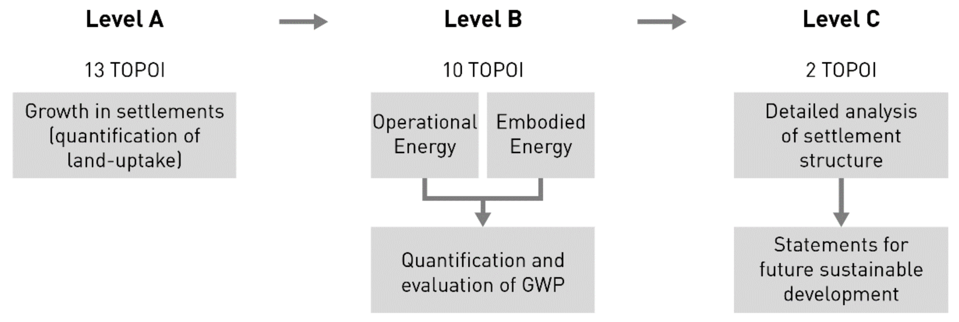
The study applies the TOPOI [2] settlement types as an analytical framework to show patterns of energy and resource usage. The data set TOPOI—Urban Rural Settlement Types—Version 1.0 [53], is a geospatial classification of urban and rural settlement types in Lower Saxony, as described in Section 2.

4. Method

The analysis is carried out in four steps, described in the following. In step 1 and 2, the key data are generated which is superposed to the TOPOI settlement types in step 3 (see Figure 2). In step 4, the latter are analysed with a view to resources and energy in a three-level evaluation framework (see Figure 3).

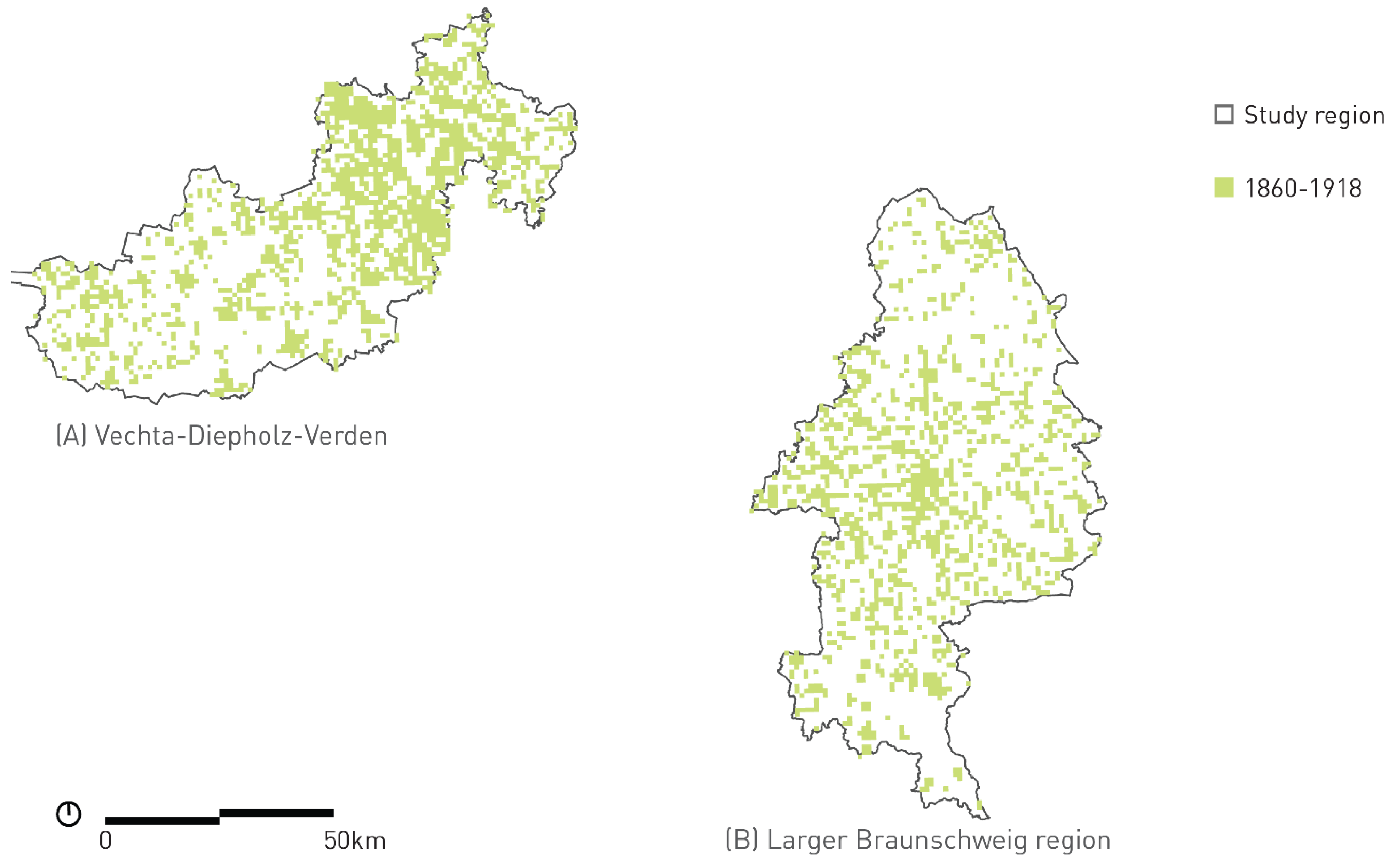
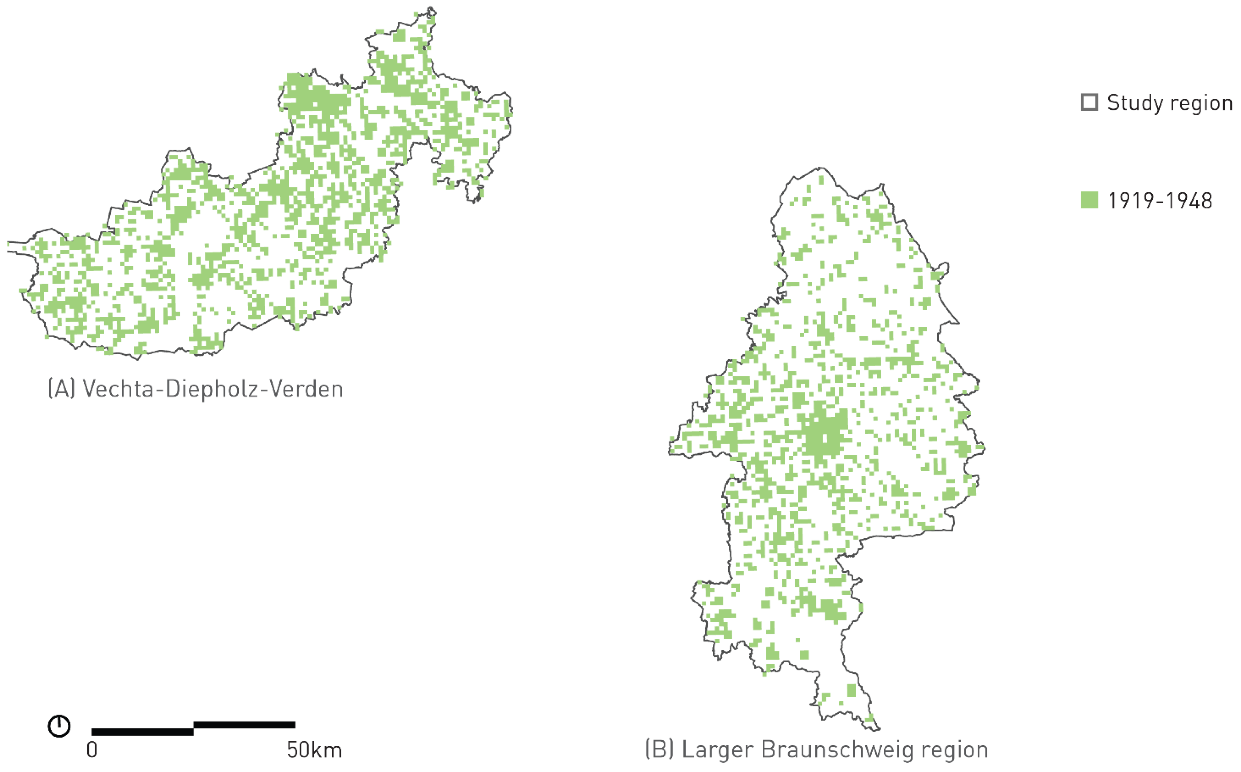
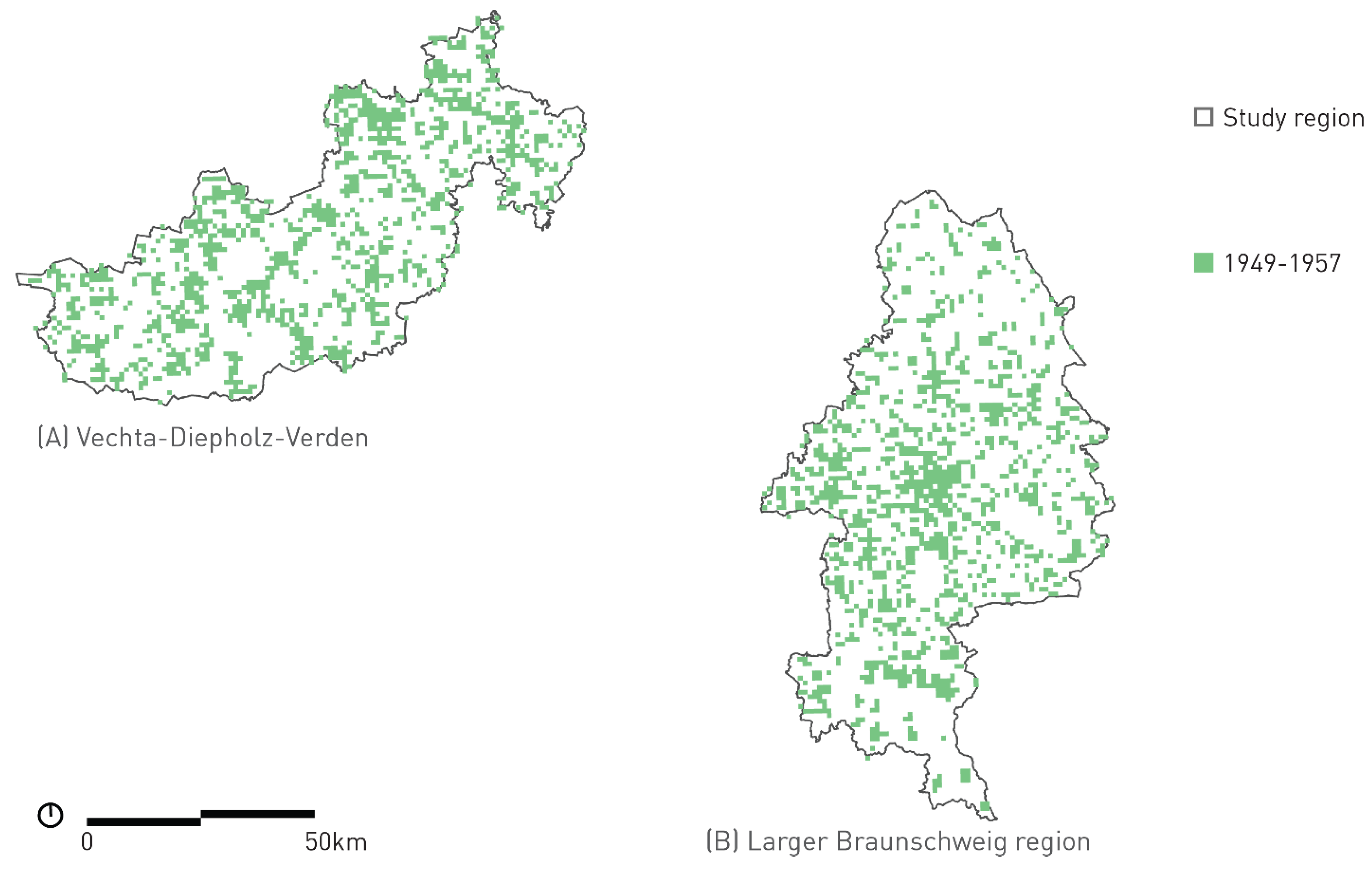
4.1. Temporal–Spatial Dynamics of Growth

In a first step, a dataset based on the 2011 German Census data [32] was built to show the growth of the residential area (residential building and open spaces area as per definition in [54]) in hectare in the different building periods defined in TABULA (see Section 3.1, [39]). A residential area is a structurally shaped area including the associated open space (courtyard area, house garden), which is used exclusively or predominantly for residential purposes [18,54]. The calculation of land-uptake is based on the growth of the number of residential buildings [32] in the respective time period multiplied by the average “residential building and open space area” per building (909 m²) in Lower Saxony in 2015 [55]. These numbers are visualized using the census grid with the aim to show the temporal–spatial dynamics of growth.

4.2. Calculation of Global Warming Potential (GWP)

The investigation uses the global warming potential (GWP) to compare different aspects of sustainability. As described before, life cycle analyses are used as the database to evaluate the GWP. Within this research framework, only the energy for the construction phase, use phase and maintenance are considered, excluding disposal or reuse, because the actual status of the building stock should be represented. In combination with identified settlement types, the embodied energy in existing residential buildings and the energy consumption during operation can be rated as properties of each TOPOI type. In order to compare the results, they are calculated per year. Regarding the embodied energy, the calculations are based on a lifecycle of 50 years, which means that the energy already used for the construction of the building is divided by 50 years for the whole life cycle. Furthermore, the embodied energy in all streets and roads is considered. To rate the GWP, all calculations results are expressed in CO₂ equivalents, based on GEMIS 4.95 [56] for the energy supply and Ökobaudat 2016 [41] for construction and maintenance for existing residential buildings.

4.3. Superposition of the Generated Key Data with the TOPOI Settlement Units

In order to perform in-depth analysis for different settlement units along the urban–rural gradient, the results from Section 4.1 and Section 4.2 were superposed with the TOPOI settlement units. TOPOI, by their formative process, do not conform to grid systems. When the data describing the building stock and the TOPOI borders do not perfectly align, situations occur where multiple TOPOI are within a 1 km grid cell. Therefore, the existing data on the building stock (2011 German Census [32]) has been transferred from the 1 km grid (see Section 3.3) to the TOPOI. First, the TOPOI were split into smaller parts using the given 1-kilometre grid as a cutting mask. In the next step, procedures for two possible scenarios are applied: (1) when a grid cell contains parts of only one TOPOS (single settlement unit of a specific settlement type) the data values can simply be transferred from grid cell to the respective TOPOS piece at a 1:1 ratio; (2) when a grid cell contains parts of multiple TOPOI (more than one settlement unit of a specific or different settlement types) within the same grid cell, a procedure to distribute the data values proportionally is conducted. For this purpose, the total area of building footprints [35] that are located within residential areas according to ATKIS [36,37] is calculated for each TOPOI piece in that grid cell. Next, for each grid cell, the sum of residential building footprints within the cell is calculated and the proportional share for each piece of TOPOI located within the grid cell is determined. Based on this share, the grid cell data are distributed to the respective piece of the TOPOI. In situations where a part of a TOPOS constitutes 90% or greater than the total area of the residential building footprints of a grid cell, that TOPOS is given 100% of the data of that grid cell. After the data values have been distributed to all pieces of the TOPOI, they are re-joined and overall growth per time period and the sum of the LCA data is calculated.

4.4. Evaluation Framework

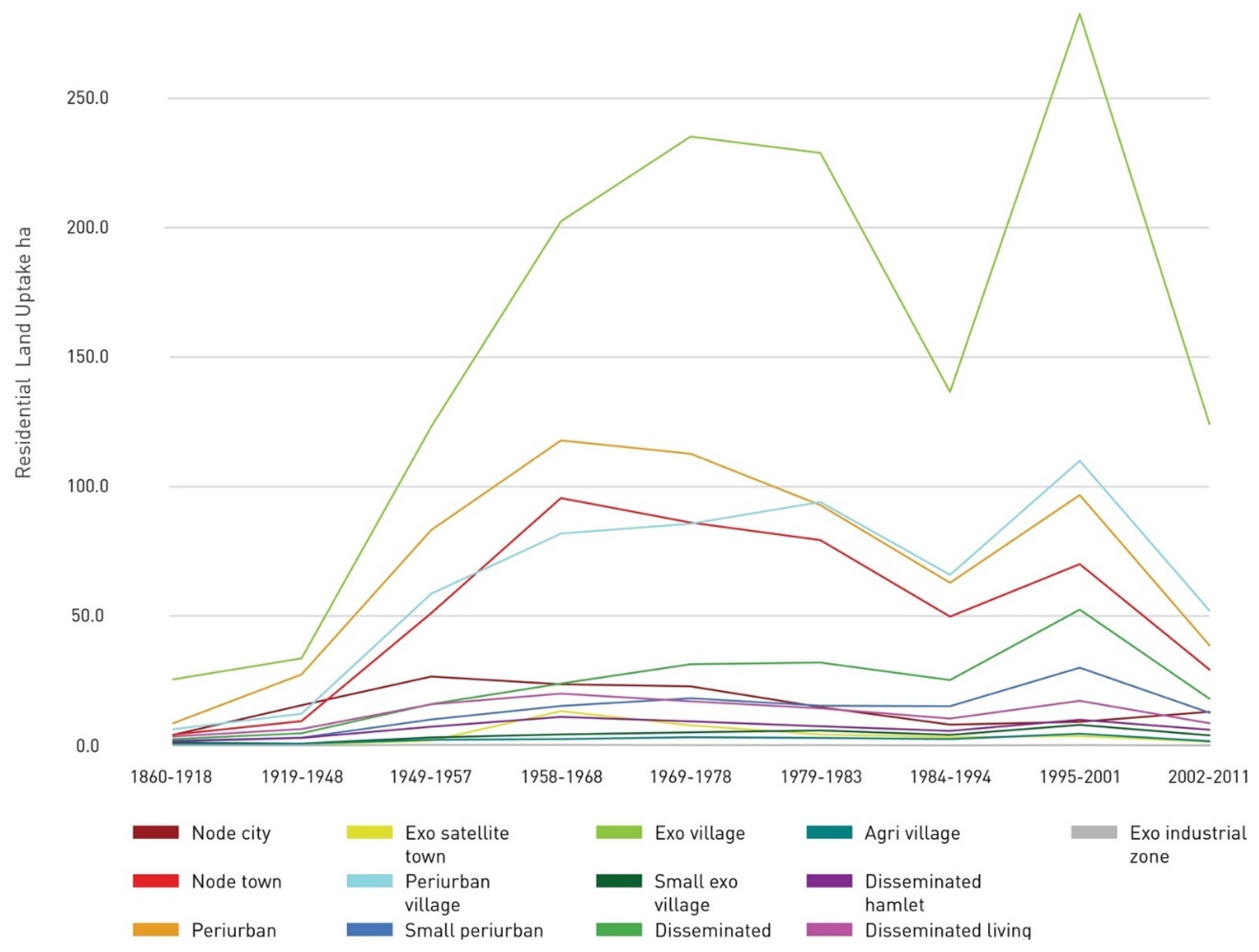
The evaluation framework of this study is divided into three levels of detail. The first level (Level A) focusses on the spatio-temporal growth, i.e., the correlation of specific growth patterns and land-uptake of all 13 settlement types within the study regions. Level B focuses on the quantification of energy consumption and embodied energy in different settlement typologies, calculated in CO₂-equivalents. The goal is to quantify the environmental impact of specific settlement types in order to be able to compare them and to identify the most influential TOPOI type within the study regions in terms of the GWP. In Level C, the “best case” TOPOI type with the highest negative impact will be compared with the most influential TOPOI, by using a detailed analysis of input parameters of the building stock to derive statements for future sustainable developments within the study regions.

5. Results

5.1. Results—Level A

Level A of the evaluation framework analyses the temporal–spatial dynamics of growth and quantifies the land up-take. The superposition of the data onto the TOPOI settlement units as described in Section 4.3 allows for a higher spatially resolved perspective of the data and understanding of the urban development.

The settlement area growth is visualised in Figure 4, which shows in which time period the highest growth took place per 1 km grid cell. Figure 5 (see also Table A4) describes the average land-uptake calculation based on residential buildings according to building age classes. The spatial distribution of the expansion of the settlement area for each building age class separately are shown in Figure A2, Figure A3, Figure A4, Figure A5, Figure A6, Figure A7, Figure A8, Figure A9, Figure A10, Figure A11 and Figure A12.

Due to data availability, no growth is mapped for the so-called exo-industrial zones, for example. The availability and integration of additional building types would impact the results significantly.

The main growth of residential buildings and the resulting land-uptake between 1919 and 2011 has taken place in the TOPOI types node city (n = 1; 1629.7 ha, 4.65% of total growth), node towns (n = 7; 4190.7 ha, 11.95% of total growth), periurban towns (n = 24; 6089.9 ha, 17.37% of total growth), periurban village (n = 42; 4935.3 ha, 14.80% of total growth) and most clearly the exo villages (n = 524; 12,667.6 ha, 36.13% of total growth). After steady growth in the first half of the 20th century, the main growth in the node city (Braunschweig) took place after the second World War with 22.6 ha annually between 1949 and 1978, with its peak between 1949 and 1957 (26.6 ha/a).

Likewise, a large increase in area growth occurs in node towns (peak: 1958 to 1968 with 95.6 ha/a), periurban towns (Peak: 1958 to 1968 with 117.8 ha/a), periurban villages (peak: 1979 to 1983 with 94.0 ha/a) and exo villages (peak: 1969 to 1978 with 235.2 ha/a) in the post-war period. After comparably lower growth in the period between 1984 and 1994, there was a strong increase after German reunification in the period between 1995 and 2001.

The exo village, with an increase of 282.6 ha/a, stands out in particular. This TOPOI type is characterised by both its isolated location and high functional density. It is predominantly located in study region (B), the larger Braunschweig region. The considerably higher land-uptake for this TOPOI type (1919–2011: 111.9 km² compared to 13.9–55.9 km² for the aforementioned types) is related on the one hand to the number of settlements of this type (n = 524) as can be seen in the numbers for the median growth across the time periods 1919–2011: exo villages 1.4 ha compared to 10.6/23.6 ha for the periurban villages/periurban towns and 59.5/154.8 ha for the node towns/node city.

In the further analysis considering additional data on population and building density, it is revealed that there are fundamental differences with regard to the relationship of the surface area in relation to population size and density as well as the building density (see Figure 6; Table 3 for definitions of the indicators). For example, that the exo satellite towns have the highest residential building density (RBD) and population density (PD) while residential land-uptake (RLU) is very low. In contrast, it can be seen for the exo village, for example, that we have a relatively high RBD combined with a very high total RLU and a low PD. Noticeable is the low median RLU. Within the set of TOPOI types, population density in exo villages ranks 7th, yet with a high density of residential buildings. The same is visible for the periurban village (8th) and periurban town (9th) as well as the node town (10th). This allows conclusions to be drawn that these are low-density settlement types such as single-family and terraced houses. For the node city, the densities for population and residential buildings both align at a high level. The exo satellite town has the highest population and housing density, while land consumption is very low.

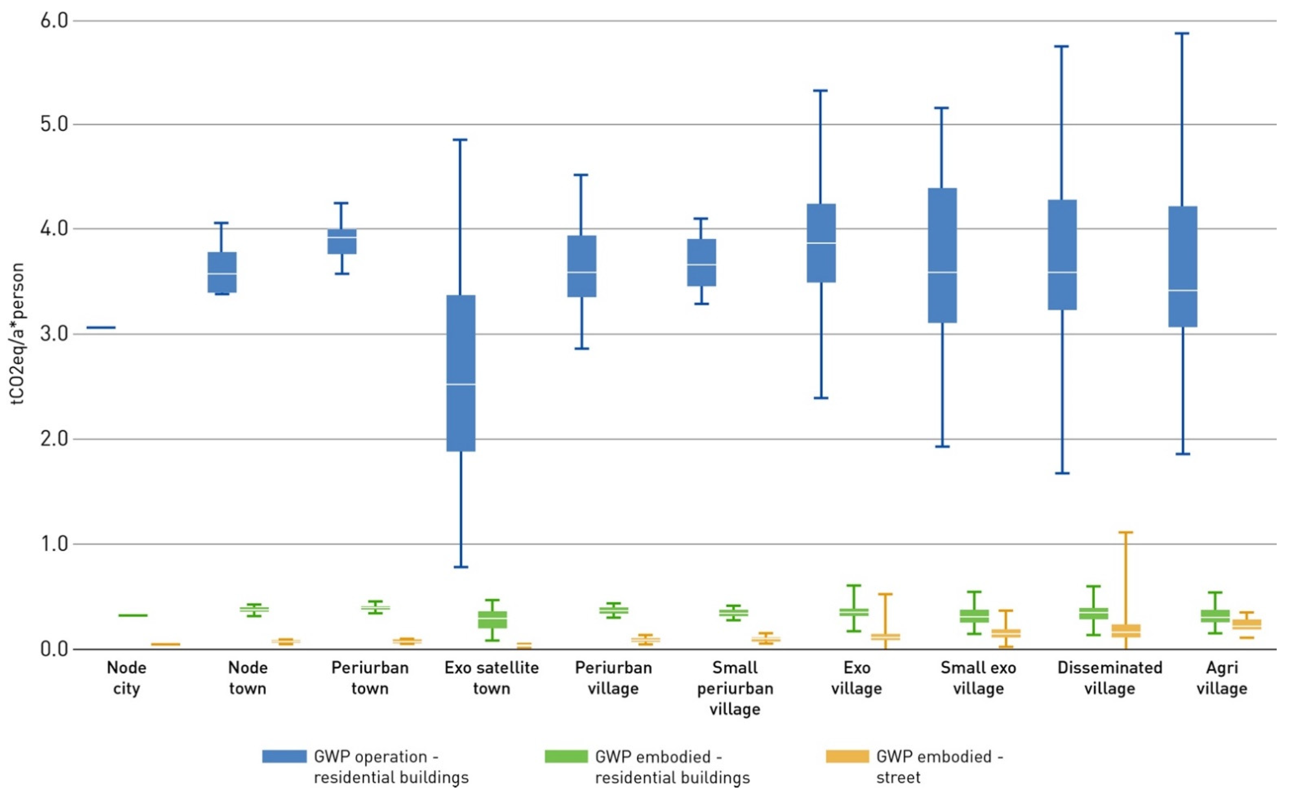
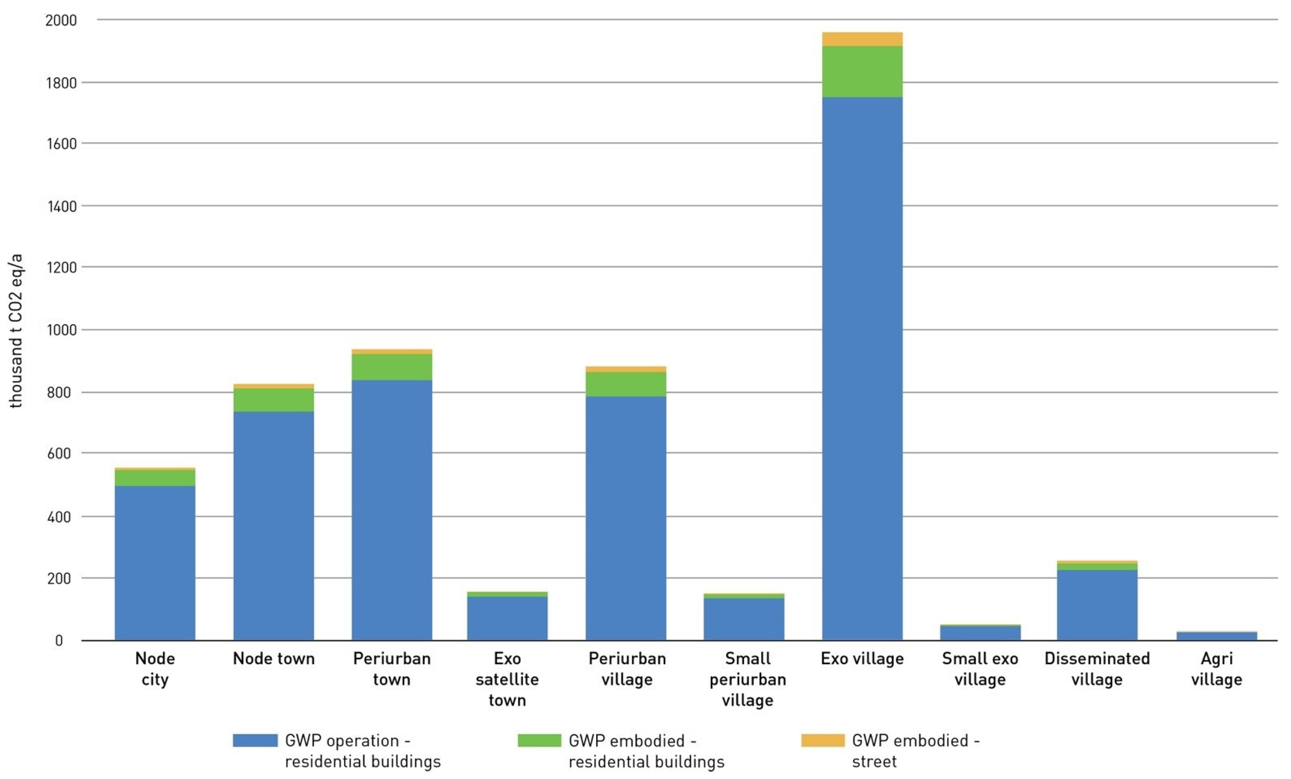
5.2. Results—Level B

Results on Level B include the evaluation of the GWP for different settlement types by creating box plots. The box plot method is very suitable for a large number of numeric data, as is divides all data in quartiles and hereby displays the information with five numbers: minimum, 1st quartile, median, 3rd quartile and maximum. The initial box plot evaluation for all 13 TOPOI had to be reduced to 10 TOPOI: as only residential buildings are considered, the exo industrial zone had to be eliminated. Furthermore, two TOPOI (disseminated hamlet and disseminated living agri hamlet) had very differing values and the interquartile ranges (IQR) were too high to see significant results.

As the data of the census in combination with life cycle data include approximations and inaccuracies, the outliers have been removed to focus on the most frequently occurring data. To compare the GWP of embodied energy with the GWP during operation, the results are expressed per year and person. The division by person (inhabitants) offers the comparison of all settlement types, as the population density is essential to rate the GWP in terms of sustainability. Figure 7 shows the results for the GWP per year and person, divided into operational and embodied emissions.

The distribution of GWP for the operation of a building reaches an average higher level than the embodied energy. The median of different settlement types for emissions during operation ranges from 2.57 t CO₂ eq/a*p (exo satellite town) to 3.97 t CO₂ eq/a*p (periurban town). The difference of 1.4 t CO₂ eq/a*p is very meaningful, taking the overall goal of the German government into account to reduce the greenhouse gas emissions until 2050 by 80% to 95% compared to 1990 [57]. Starting by around 12.5 t CO₂ eq/a*p in 1990, the goal for 2050 would lead to less than 1 t CO₂ eq/a*p including mobility, nutrition and all general consumptions of a person [58,59].

The distribution of CO₂ equivalent emissions for the construction and maintenance of buildings is, compared to the emissions during the operation of a building, quite small with fewer deviations. The median of embodied emissions per year and person ranges from 0.29 t CO₂ eq/a*p (exo satellite town) to 0.39 t CO₂ eq/a*p (periurban town). The deviation of 0.1 t CO₂ eq/a*p has a small impact. This shows that the median embodied energy per person in buildings does not vary a lot with different settlement types.

The embodied energy in streets can also be displayed as GWP per person and year. The evaluation in a box plot diagram shows the rising impact of GWP in streets with increasing rural location of the settlement type. The agri village as the most rural TOPOS results in a median of 0.22 t CO₂ eq/a*p, while the node city has a median of 0.05 t CO₂ eq/a*p. Nevertheless, in comparison to the emissions of buildings, the impact of the embodied energy in streets is rather small.

By rating the values of embodied emissions in terms of sustainability, it has to be kept in mind that the expression of values per year is a way to make embodied emissions comparable to, in this case, operational emissions that occur every year. Actually, the building stock and streets are already built and the energy has been used years ago.

The evaluations show that the settlement type exo satellite town has the smallest environmental impact, compared to the other TOPOI types. Therefore, the next research level will, on the one hand, focus on exo satellite towns and their attributes and properties, following the question, what can be learned from this settlement type and adapted for other or future settlements. Taking a closer look at the impact of all residential buildings and streets in the study regions will help to identify settlement types with a large impact. Figure 8 shows the total GWP for buildings and streets for the status of 2011.

Exo villages have by far the largest environmental impact. Around 40% of all residential buildings are built in exo villages, with more than 30% of all residents within the study regions. The analysis per person also showed that exo villages are one of the settlement types with a higher GWP (Figure 7).

5.3. Results—Level C

The results of the analysis in Level B form the basis for Level C, in which the best-case settlement exo satellite town will be analysed in detail and compared with the exo villages. The latter have an average size of 42 ha with a total building density of 13.1 buildings/ha, population density of 14.0 inhabitants/ha and an open space ratio at 86.8%. They are characterised by their high number of functions, including a small percentage of agricultural buildings, while the retail ratio is very low. The settlement units around exo villages are few and the connectivity to other settlement units is low. Exo satellite towns have the highest population density of all TOPOI types with 48.2 inhabitants/ha (median) at an average size of 81 ha with a total building density of 10.9 buildings/ha and an open space ratio at 82.8%. They can be considered the suburban developments to the periurban towns due to their proximity and transport links to the same. However, exo satellite towns still have a high functional diversity (see also Table A2 and Table A3).

Exo villages have the highest environmental impact in terms of total GWP (embodied energy + operational energy + streets) in the study regions (Figure 8), while exo satellite towns have the lowest GWP per person (Figure 7). The research aims at identifying significant input parameters which lead to the lower GWP per person for exo satellite towns in comparison to exo villages. As the calculations are based on construction year classes and building typologies, the distribution for both is evaluated. Due to the results on Level B (see Figure 7) the following analysis will focus on the operational emissions, since this is the biggest impact compared to embodied energy in buildings and streets.

The residential building stock of the study regions is dominated by single-family houses (SFHs) (67%) and terraced houses (THs) (21%). The share of multi-family houses (MFHs) is 12% and apartment blocks (ABs) contribute only 0.4%. The distribution of different building typologies within a settlement type is essential for the GWP, as building dimension and volume in combination with number of apartments correlate directly. For example, a single-family house built in the 1960s has around 20% more CO₂ eq/m²a compared to a multi-family house in the same construction year class. Figure 9 shows the distribution of all residential buildings and the corresponding GWP (t CO₂ eq/a).

There are significant differences of both settlement types in terms of building typologies. SFHs, THs and MFHs have almost equal shares within exo satellite towns, while SFHs dominate exo villages with 76%. There are no ABs and very few multi-family houses in exo villages. The distribution of GWP in exo villages correlates almost directly with the building count, while the MFHs (44%) have the biggest environmental impact in terms of GWP in exo satellite towns, followed by ABs (36%). This shows that the relation between building typology and GWP is different in both settlement types, which leads to the assumption that the construction year, as another input parameter of the calculation, varies as well between both settlement types.

In the following paragraph, the building stock will be analysed regarding construction year classes, using the division in five groups. The construction year classes are distributed to buildings built pre-war (until 1948) and post-war (1949–1978) on the one hand and assigned to different regulations concerning thermal insulation and energy saving ordinance on the other hand. The first thermal insulation ordinance (WSVO) was adopted in 1977 with restrictions on maximum values for heat transmission coefficients for exterior building components [60]. Six years later in 1984, this regulation was revised with more strict regulations for heat transmission coefficients. From today’s point of view, the change of 1.75 W/m²K (in 1977) to 1.5 W/m²K (in 1984) for exterior walls and 3.4 W/m²K to 3.1 W/m²K for windows is no significant difference [61], putting it in relation to today’s requested values of 0.28 W/m²K for exterior walls and 1.3 W/m²K for windows (EnEV 2009) [62]. In 1995, the updated WSVO introduced a new method to compare heat losses by transmission and ventilation with heat gains from internal loads and solar radiation. Using this method, the annual heating requirement for a whole building was calculated, and not only heat losses through exterior components were considered [63]. As this method is a more comprehensive approach and it was the base for today’s energy saving regulation, 1995 is considered as the “real” beginning of energy efficient buildings, besides the thermal insulation ordinance a heating appliance ordinance (HeizAnlV) that existed with the first version in 1978 [64]. In 2002, the first energy saving ordinance (EnEV) was introduced, which combined both the WSVO and HeizAnlV, and apart from the annual heating requirements, also calculated the primary energy consumption [65]. The EnEV was revised four times until 2011 (research framework) [62]. The classification of the 11 construction year classes into five groups is shown in Table 4 and is chosen to evaluate the existing building stock in terms of energy consumption levels.

Within the study regions, more than 60% of all residential buildings were built before the first thermal insulation ordinance and 80% before the revised version in 1995. The distribution of building ages in exo satellite towns and exo villages are shown in Figure 10.

The majority of residential buildings in exo satellite towns are post-war buildings (65%), built between 1949 and 1978. Only 32% have been built after the first thermal insulation ordinance, which cause 20% of GWP during operation. The environmental impact of 65% post-war buildings is more significant and responsible for 78% of CO₂ emissions during operation. The distribution of building types within the dominating construction year class correlates to the distribution of building types in the whole TOPOI type. There are only a few less SFHs and more MFHs built post-war.

The share of pre-war buildings in exo villages is higher (21%) compared to exo satellite towns, though in general, more buildings were built after the first thermal insulation ordinance (40%). This share of “new buildings” produces 33% of all CO₂ emissions during operation, while post-war buildings are responsible for 40% GWP and pre-war buildings, for 27% GWP. The distribution of building types in pre- and post-war classes correlates with the distribution within the whole settlement type, despite a slight deviation to a higher share of SFHs and THs and less MFHs.

The analysis of construction year classes shows that both settlement types are dominated by old buildings. Comparing the environmental impact in terms of GWP reveals that the distribution of building types within a construction year class has a significant impact on CO₂ emissions.

6. Discussion

The development of strategies for the sustainable retrofitting of existing settlement units and their building stock, as well as the sustainable development of new areas, requires a comprehensive understanding of the interrelationships between resource and energy demands together with the form and structure of settlement units. The building-type-based analysis built on the census data allows a spatially explicit analysis across scales based on the TOPOI types. Hence, a number of conclusions can be drawn:

Particular TOPOI types, especially the exo villages, are largely responsible for high resource and energy consumption in both study regions. These are characterised by a low population and building density. This can be attributed to the developments of residential extensions dominated by detached and terraced houses. It is striking that this overall high negative effect is the result of rather small developments of each individual settlement unit throughout the years. Due to the lack of a region-wide integrated evaluation approach in urban land use planning, the extent of the negative impacts does not become apparent at first. For sustainable development, such a comprehensive perspective in approval processes is indispensable from the authors’ point of view. The method presented here offers the possibility to do so.

A notable observation in the course of the study is the exo satellite town, which stands out positively in terms of both land consumption in relation to population density and GWP. Exo satellite towns are large-scale, master-planned high-density urban extensions developed as mass housing estates in the 1960s and 1970s.

The results of the detailed analysis of exo satellite towns and exo villages (see Section 5.3) lead to the conclusion that the biggest differences between both are the population density, distribution of building types and the share of pre-war buildings. A redensification of existing neighbourhoods in exo villages would theoretically lead to a reduction in the GWP per person. In this context, it is important to mention the challenge of redensification strategies in existing neighborhoods with mostly single-family houses—also in terms of embracing existing structures and their embodied energy. However, the need for denser development patterns for a sustainable growth of new settlement areas is becoming evident through this analysis.

For the existing building stock, a potential approach would be the extensive renovation on up-to-date building standards (EnEV), taking residential buildings built before 1995 into account. However, the following shows that the renovation approach cannot deliver the necessary reductions for the most significant settlement type within the study regions. A scenario with 100% renovated SFHs and THs by 2050 (in consideration of the non-renovatable building stock due to heritage purposes), which would be a renovation rate of 2.4% per year and a continuing renovation rate of 1% for MFHs leads approximately to a reduction of around −0.6 t CO₂ eq./pers*a (3.3 t CO₂ eq./pers*a) for exo villages. A renovation approach including 100% renovated residential buildings (all building types) in exo villages would result in a reduction of around −0.7 t CO₂ eq/pers*a (3.2 t CO₂ eq./pers*a). This result reflects the evaluation of Section 5.3, that SFHs are the main driver within exo villages. Taking into consideration that only SFHs will be renovated, a reduction of −1.0 CO₂ eq/pers*a (2.9 t CO₂ eq./pers*a) is possible by using a higher renovation standard than the regulation (EnEV) demands. Besides the higher reduction in energy consumption, the use of material would increase, and therefore the embodied energy. It also needs to be mentioned that no costs or social aspects are considered in this study.

The overall governmental goals for 2050 request total reductions in greenhouse gas emissions of 95% [57], which leads to around 200 kg CO₂ eq/pers*a for buildings. To achieve significant impacts to reduce the GWP, the stated reductions would need to go along with a change in the energy supply. Taking 2050 scenarios for energy supply into account, the share of renewable energies will dominate the system, which will reduce the GWP per person in residential buildings significantly. However, a study on energy supply scenarios is not part of this article.

The introduced method to identify main drivers in terms of land-uptake and global warming potential on the level of the region and settlement units offers evaluations that are based on classifications and assumptions. Using the method, an extrapolation for the whole residential building stock in Germany is possible, provided that appropriate data are available. Working on a large scale, the results are representative and general statements are possible. Nevertheless, there are some restrictions that have to be kept in mind.

The data about the existing building stock are based on the German Census 2011, which is missing ten years to today’s status of the building stock. As the analysis has shown, new buildings have a small share within the study regions and the rate of new constructions of residential buildings in Lower Saxony from 2011 to 2019 was an average of 0.6% per year [21]. For this reason, the missing numbers of the last ten years may not have a major impact on the overall result. For a conclusive assessment of this impact, the study needs to be carried out again with data from the new German Census planned for 2022.

Due to the limitations of the available dataset, the analysis of the temporal–spatial dynamics of growth as well as GWP is based on residential buildings only and thereby does not include, for example, industrial buildings and linked land-uptake. The study does not address the potential consequences of land-uptake, for example, in terms of ecosystems.

Furthermore, the calculations on residential buildings are based on generalised types and classifications. The distribution of buildings across multiple settlement units within each 1 km² grid cell is carried out proportionally, possibly leading to some bias when distributing the data by area. As the building data used are accumulated on the 1 km grid, there is no way to more precisely pinpoint the buildings’ exact location. The calculations of energy consumption during operation are based on benchmarks, combined with statistic data for energy supply shares in Lower Saxony, which also is a simplification. The life cycle assessments to evaluate the embodied energy are based on the Ökobaudat 2016, which includes data on how a building would be built today. The way of transport or construction processes in the actual construction year class, for example in 1860, might have been different. The building constructions are based on assumptions and classification and represent an approximation.

Life cycle assessments result in a number of environmental indicators, e.g., GWP, primary energy consumption, ozone depletion potential or acidification potential. This study evaluates only the GWP, as CO₂ emissions often are the focus of political statements or regulations. Nevertheless, other environmental indicator assessments would be necessary for a holistic life cycle analysis.

The embodied energy has been excluded in the detailed evaluations of this study. The chosen method to express the GWP per year and person is a valid way to compare different settlement types by including population density. The expression of embodied energy per year and person for existing buildings is questionable though, as the buildings have already been built and the energy used for construction cannot be changed. Therefore, the consideration of embodied energy is more significant for new buildings or regarding the question of demolition versus renovation. As new buildings are built more energy efficient, the significance of embodied energy is increasing. A building built in 2015 has a share of 40% embodied energy only for the construction of the building. In 2009, which represents almost the newest buildings within this study, the share of embodied energy was only 30% [25]. This trend shows that the impact of embodied energy is increasing and needs to be included in holistic approaches for new buildings.

Author Contributions

Conceptualization, A.-K.M., E.E., O.M., O.R., R.Z. and V.M.C.; methodology, A.-K.M., O.M., R.Z. and V.M.C.; investigation, A.-K.M., O.M. and R.Z.; writing—original draft preparation, A.-K.M. and O.M.; writing—review and editing, E.E. and V.M.C.; visualization, A.-K.M. and R.Z.; supervision, E.E. and V.M.C.; funding acquisition, V.M.C. and O.M. All authors have read and agreed to the published version of the manuscript.

Funding

This research was funded by the Ministry of Science and Culture of Lower Saxony and by the Volkswagen Foundation under Grant ZN3121.

Institutional Review Board Statement

Not applicable.

Informed Consent Statement

Not applicable.

Data Availability Statement

The TOPOI–Urban Rural Settlement Types–Version 1.0 is openly available in the Digital Library Institutional Repository of TU Braunschweig at doi:10.24355/dbbs.084-202003180800-0. The data on global warming potential and land-uptake presented in this study is available on request from the corresponding author. These data are not publicly available due to privacy reasons of the special evaluation of base data on building stock obtained from the State Office for Statistics Lower Saxony.

Acknowledgments

We acknowledge support by the German Research Foundation and the Open Access Publication Funds of Technische Universität Braunschweig.

Conflicts of Interest

The authors declare no conflict of interest.

Appendix A

Table A1. Range of eleven indicators of form, function, and spatial linkages used in the affinity propagation clustering for classifying settlement types according to the TOPOI method [2].

FORM	Min.	Max.
Area (A) The is the area of a settlement unit in ha.	0.84 ha	3662.06 ha
Compactness (C) The compactness of a settlement unit is calculated: C = 2 √πA⁄P*100(%); C = compactness, A = area, P = perimeter [66].	14%	99%
Building Density (BD) BD is the number of buildings in each settlement unit divided by the area A (ha).	0.82 buildings/ha	32.36 buildings/ha
Open Space Ratio (OSR) OSR describes the amount of space that is not occupied by built structures within a certain area. OSR is calculated by applying the formula: OSR = A–BA; A = area, BA = Built up area.	45.74%	99.74%
FUNCTION
Functional Richness (FR) FR describes the presence of different functions in a settlement unit ranging from 1 to 8 available functions here (residential area; retail and services; public facilities; industrial and commercial area; agricultural facilities; supply facilities; disposal facilities; parks, sport and recreation facilities)	0	8
Population Density (PD) PD is the number of inhabitants per hectare. The data source gives the absolute number of inhabitants per 1 ha cell (yz). The sum of the total population per cell within one settlement unit is divided by the area (A).	0.00 inhabitants/ha	83.32 inhabitants /ha
Retail and Services Ratio (RSR) RSR is the percentage of the area A with retail and services per unit.	0.00%	92.85%
Agricultural Facilities Ratio (AFR) AFR is the percentage of the area A with agricultural facilities within each unit.	0.00%	89.88%
SPATIAL LINKAGES
Settlement Density (SD) The density of settlement units assesses the number of units within a 3 km radius, using the Euclidean distance between centroids.	1	71
Public Transport Connectivity (PTC) PTC is the number of settlement units directly linked to each other by public transport. It can be calculated as PTC = ΣL (L₁ + L₂ + L_n) where L is the number of unique settlement units reached by each public transit line that goes through a TOPOI.	0	76
Proximity to Regional Train Station (PRTS) The proximity to (operating) regional train stations calculates the shortest distance along the street network between a regional train station and the centroid of each settlement unit in km [37,67,68,69].	0.00269 km	28.11 km

Table A2. The TOPOI for the two study regions in Lower Saxony (Germany) and the median per indicator. The order of the TOPOI in the table develops along the population density, with the exception of “exo satellite town”, which is subordinated to Node City and Periurban Town [2].

TOPOI	Unit Count	Indicators
		Form				Function				Linkages
		Area (ha)	Compactness (%)	Building Density (buildings/ha)	Open Space Ratio (%)	Functional Richness	Population Density (inhabitans/ha)	Retail and Services Ratio (%)	Agricultural Facilities Ratio (%)	Settlement Density	Public Transport Connectivity	Proximity to Regional Train Station (m)
Node city	1	3662	14%	13.9	80%	8	43.5	8.9%	0.3%	4	68	2669
Node town	7	1153	22%	15.5	81.8%	8	22.5	5.8%	1.6%	18	31	1649
Periurban town	24	526	29%	14.4	82.8%	8	21.4	5.8%	1.0%	23	23	1407
Exo satellite town	9	81	61%	10.9	82.9%	7	48.2	2.3%	0.1%	13	3	3920
Periurban village	42	224	38%	15.2	84.5%	8	19.7	4.8%	2.3%	13	21	1665
Small periurban village	37	53	60%	15.1	86.6%	7	17.2	1.7%	5.0%	13	18	3654
Exo village	524	42	63%	13.1	86.8%	7	14.0	1.4%	7.3%	10	5	6559
Small exo village	73	14	76%	11.3	88.6%	4	11.0	0.0%	13.4%	11	6	6172
Disseminated village	160	27	53%	8	90.2%	6	7.2	2.1%	8.6%	44	10	8851
Agri village	35	20	58%	7.7	89.6%	5	5.2	1.4%	14.2%	12	23	8440
Disseminated hamlet	1071	4	81%	4.5	91.4%	3	2.3	0.0%	0.0%	34	0	7017
Disseminated living agri hamlet	4283	3	89%	4.7	92.6%	2	2.3	0.0%	23.9%	38	0	8098
Exo industrial zone	35	18	69%	1.9	68.6%	3	0.0	0.0%	0.0%	15	0	3779

Table A3. Description of the thirteen TOPOI identified in the two study regions. The given TOPOI exemplars result from affinity propagation clustering [2].

TOPOI Description	Exemplary TOPOI Map
Node city (n = 1) In the two study regions, only one node city was identified (Braunschweig). Due to its physical form, comprising large un-built areas, such as parks, this TOPOS is large but the least compact agglomeration. The node city TOPOS has the highest count of public transport connections: no other TOPOI are so well connected to other settlement units, even though its dimension increases the distance to the closest regional train station and decreases the amount of settlement units in its surroundings (3 km radius). The retail ratio is highest in comparison to other TOPOI. In the two study regions, the node city shows a high diversity of functions and large number of buildings, and the population density (43 inhabitants/ha) is the second highest of all TOPOI.
Node town (n = 7) Node towns are the second least compact TOPOI. They feature a high diversity of functions. Their public transport connectivity and population density are around half of that of a node city. The settlement density in a 3 km radius is much higher than in node cities. The distance to a regional train station, measured from the centroid, is less than 2 km, which means that these settlement units are strategically well located with respect to public transport. In comparison to a node city, these settlement units have a lower retail ratio.
Periurban town (n = 24) Periurban towns are well connected to node cities and node towns. Since they are relatively small, they feature relatively short distances to regional train stations, which are comfortably reachable on foot or by bike from within the given settlement unit. Periurban towns are comparatively smaller than node towns but have not significantly different characteristics with respect to functional richness and retail ratio. They are slightly smaller in other indicators, such as population density, building density and slightly bigger in terms of open space ratio. Additionally, in comparison to node towns, periurban towns have fewer connections to other settlement units via public transport.
Exo satellite towns (n = 9) Exo satellite towns have the highest population density (median of 48 inhabitants/ha) They have a very low connectivity by public transport and their distance to a regional train station is with more than 4 km relatively high. Due to their proximity and transport connectivity to periurban towns, they can be considered as their suburban developments, predominantly characterized by housing. However, exo satellite towns still have a high functional diversity.
Periurban village (n = 42) The periurban villages have a relatively high ratio of retail and a high functional richness. The accessibility to a regional train station is—in comparison to the (larger) size of other settlement units—a very high (median 1.7 km). This means, from within a periurban village, regional train stations are comfortably reachable on foot and by bike. In general, the connectivity by public transport is almost as high as that of periurban towns. Amongst all other village types, the periurban villages are the least compact.
Small periurban village (n = 37) Small periurban villages have on average a medium number of connections by public transport and also diversified functions. These settlement units have the highest average building density. The presence of retail and agricultural buildings in particular in small percentages contributes to their village status.
Exo village (n = 524) An exo village is generally located more than 6 km from a regional train station. They have a high number of functions, including a small percentage of agricultural buildings, while the retail ratio is very low. The settlement units around exo villages are few and the connectivity to other settlement units is low. Exo villages are mostly found in the larger Braunschweig region. In the region Vechta-Diepholz-Verden, they appear close to periurban towns.
Small exo village (count 73) Small exo villages are very isolated with a large distance to a station and limited access to public transport. They are in average 14 ha big, have no retail function, and a generally low functional richness. The share of agricultural buildings is comparatively high with 13% on average.
Disseminated village (n = 160) Most of the disseminated villages are part of a dense fine-meshed network (median: 44 units within 3 km) of villages and characterized by a large remoteness. The connectivity is low and the distance to the railway station is the highest compared to all other TOPOI with almost 9 km. The comparatively high proportion of farm buildings of almost 9% of the surface area indicates its agricultural character.
Agri village (n = 35) Agri villages are characterized by a comparatively high proportion (14.2% of the total area) of agricultural facilities. They are located rather far from other settlement units and railway stations but have good connections to the bus-based public transport network.
Disseminated hamlet (n = 1071) This TOPOS consists of a large group of units. Access is only possible via individual mobility. They have a low number of functions and no retail. However, disseminated hamlets have a big number of other settlements around.
Disseminated living agri hamlet (n = 4283) Disseminated living agri hamlets form the biggest TOPOI group and are mostly found in the region of Vechta-Diepholz-Verden. They feature mainly two functions: agriculture and living, and they are finely dispersed within a dense network of hamlets (median: 38 units within 3 km). There are no public transport options available.

Table A4. Spatio-temporal growth: land-uptake in hectares based on residential buildings according to building age classes and associated areas without transport infrastructure per TOPOI type (TOTAL = total growth per building age class; averages: 1st quartile, median, 3rd quartile).

			Building Age Class
			1860–1918	1919–1948	1949–1957	1958–1968	1969–1978	1979–1983	1984–1994	1995–2001	2002–2009	2010–2011
TOPOI	Count		Land-Uptake Residential Buildings ¹ (ha)
Node City	1	TOTAL	236.8	448.5	212.9	236.5	205.1	59.1	79.9	54.7	90.8	5.4
Node Town	7	TOTAL	241.0	272.4	408.6	955.8	774.4	317.3	497.3	420.4	266.3	37.2
		1st Quartile	15.3	25.9	39.2	83.7	87.2	40.1	51.0	45.9	37.5	2.4
		Median	33.8	37.2	45.7	120.6	109.2	43.8	68.9	63.3	42.9	4.3
		3rd Quartile	43.1	46.8	86.2	173.4	139.0	52.3	76.6	76.0	45.1	8.7
Periurban Town	24	TOTAL	495.4	795.6	665.9	1.178.2	1.013.9	371.5	627.9	580.3	332.1	29.2
		1st Quartile	5.5	12.9	15.2	33.8	29.2	11.1	20.4	48.3	8.5	0.3
		Median	13.3	25.3	22.5	47.1	39.2	15.7	24.6	23.3	13.5	0.8
		3rd Quartile	25.0	45.7	34.2	62.5	55.6	18.7	33.7	34.1	18.3	2.0
Periurban Village	42	TOTAL	362.6	355.5	468.9	818.3	770.5	376.0	658.7	660.1	425.8	38.8
		1st Quartile	4.4	4.1	5.5	12.3	12.9	5.4	9.9	1.1	5.6	0.1
		Median	1.0	7.5	9.0	15.8	16.5	8.5	13.3	15.5	9.1	0.5
		3rd Quartile	10.2	11.4	12.7	25.1	23.5	11.4	20.5	19.6	12.5	1.1
Exo Satellite Town	9	TOTAL	8.0	8.0	14.4	132.7	69.7	16.8	31.7	21.8	9.2	1.9
		1st Quartile	0.1	0.0	0.5	0.5	0.6	0.2	0.2	0.0	0.0	0.0
		Median	0.2	0.0	1.3	3.8	4.2	0.4	0.8	0.7	0.2	0.0
		3rd Quartile	0.3	0.4	2.5	23.8	16.1	1.3	2.9	1.2	0.7	0.1
Small Periurban Village	37	TOTAL	104.6	85.5	80.0	152.6	164.1	61.3	151.4	180.1	88.5	5.1
		1st Quartile	0.1	0.8	0.9	1.7	1.5	0.6	1.6	2.0	0.7	0.0
		Median	2.3	1.5	1.6	3.2	3.8	1.4	3.2	4.2	1.8	0.0
		3rd Quartile	3.4	2.5	3.4	6.5	5.0	2.2	5.4	7.3	4.0	0.3
Exo Village	524	TOTAL	1479.7	974.2	984.8	2024.7	2117.0	915.5	1366.1	1695.8	1049.0	60.4
		1st Quartile	0.8	0.5	0.5	1.1	1.0	0.4	0.5	0.7	0.3	0.0
		Median	2.1	1.0	1.1	2.5	2.4	1.0	1.5	1.8	1.0	0.0
		3rd Quartile	3.8	2.0	2.4	5.0	5.0	2.2	0.3	4.4	2.4	0.0
Small Exo Village	73	TOTAL	60.3	20.5	24.5	42.7	45.6	23.1	40.7	47.4	27.4	1.6
		1st Quartile	0.3	0.0	0.0	0.2	0.1	0.0	0.2	0.2	0.0	0.0
		Median	0.6	0.3	0.3	0.4	0.4	0.2	0.4	0.4	0.3	0.0
		3rd Quartile	1.2	0.4	0.5	0.9	0.7	0.4	0.7	0.7	0.4	0.0
Disseminated Village	160	TOTAL	142.9	134.8	127.4	239.1	281.9	127.9	252.2	314.6	187.3	13.6
		1st Quartile	0.3	0.3	0.1	0.3	0.2	0.0	0.1	0.2	0.0	0.0
		Median	0.5	0.5	0.4	0.7	0.8	0.3	0.6	0.7	0.5	0.0
		3rd Quartile	1.2	1.1	0.9	2.1	2.0	0.9	1.8	2.4	1.5	0.0
Agri Village	35	TOTAL	31.4	20.4	16.9	24.4	28.2	11.6	24.1	27.0	11.4	0.8
		1st Quartile	0.3	0.1	0.0	0.2	0.2	0.0	0.1	0.0	0.0	0.0
		Median	0.6	0.5	0.3	0.3	0.3	0.2	0.3	0.3	0.0	0.0
		3rd Quartile	1.2	0.9	0.5	0.8	0.7	0.5	0.7	0.7	0.3	0.0
Disseminated Hamlet	1.071	TOTAL	87.5	83.9	57.4	109.8	83.7	29.7	55.9	59.5	42.4	1.8
		1st Quartile	0.0	0.0	0.0	0.0	0.0	0.0	0.0	0.0	0.0	0.0
		Median	0.0	0.0	0.0	0.0	0.0	0.0	0.0	0.0	0.0	0.0
		3rd Quartile	0.2	0.2	0.1	0.2	0.1	0.0	0.1	0.1	0.0	0.0
Disseminated Living Agri Hamlet	4.283	TOTAL	198.5	182.8	126.6	200.4	153.0	57.4	104.0	103.0	59.8	2.4
		1st Quartile	0.0	0.0	0.0	0.0	0.0	0.0	0.0	0.0	0.0	0.0
		Median	0.0	0.0	0.0	0.0	0.0	0.0	0.0	0.0	0.0	0.0
		3rd Quartile	0.1	0.1	0.1	0.1	0.1	0.0	0.0	0.0	0.0	0.0
Exo Industrial Zone	35	TOTAL	0.9	0.9	1.2	1.5	0.8	0.3	0.0	0.6	0.1	0.0
		1st Quartile	0.0	0.0	0.0	0.0	0.0	0.0	0.0	0.0	0.0	0.0
		Median	0.0	0.0	0.0	0.0	0.0	0.0	0.0	0.0	0.0	0.0
		3rd Quartile	0.0	0.1	0.1	0.1	0.1	0.0	0.1	0.1	0.0	0.0

Figure A1. Spatio-temporal growth: annual land-uptake per TOPOI type in hectares based on residential buildings according to building age classes and associated areas without transport infrastructure.

Figure A2. Spatio-temporal growth: visualisation of the expansion of the settlement area based on residential buildings according to building age classes. Developments in the time period before 1859 are shown with a resolution (grid size) of 1 km.

Figure A3. Spatio-temporal growth: visualisation of the expansion of the settlement area based on residential buildings according to building age classes. Developments in the time period between 1860–1918 are shown with a resolution (grid size) of 1 km.

Figure A4. Spatio-temporal growth: visualisation of the expansion of the settlement area based on residential buildings according to building age classes. Developments in the time period between 1919–1948 are shown with a resolution (grid size) of 1 km.

Figure A5. Spatio-temporal growth: visualisation of the expansion of the settlement area based on residential buildings according to building age classes. Developments in the time period between 1949–1957 are shown with a resolution (grid size) of 1 km.

Figure A6. Spatio-temporal growth: visualisation of the expansion of the settlement area based on residential buildings according to building age classes. Developments in the time period between 1958–1968 are shown with a resolution (grid size) of 1 km.

Figure A7. Spatio-temporal growth: visualisation of the expansion of the settlement area based on residential buildings according to building age classes. Developments in the time period between 1969–1978 are shown with a resolution (grid size) of 1 km.

Figure A8. Spatio-temporal growth: visualisation of the expansion of the settlement area based on residential buildings according to building age classes. Developments in the time period between 1979–1983 are shown with a resolution (grid size) of 1 km.

Figure A9. Spatio-temporal growth: visualisation of the expansion of the settlement area based on residential buildings according to building age classes. Developments in the time period between 1984–1994 are shown with a resolution (grid size) of 1 km.

Figure A10. Spatio-temporal growth: visualisation of the expansion of the settlement area based on residential buildings according to building age classes. Developments in the time period between 1995–2001 are shown with a resolution (grid size) of 1 km.

Figure A11. Spatio-temporal growth: visualisation of the expansion of the settlement area based on residential buildings according to building age classes. Developments in the time period between 2002–2009 are shown with a resolution (grid size) of 1 km.

Figure A12. Spatio-temporal growth: visualisation of the expansion of the settlement area based on residential buildings according to building age classes. Developments in the time period between 2010–2011 are shown with a resolution (grid size) of 1 km.

Table A5. Street types [46]—layer structure and sizes in accordance with [47,48,49,50].

Classification		Width (m)	Driving Direction
1	motorway	12.0	1
2	trunk	12.0	1
3	primary	4.25	1
4	secondary	4.25	1
5	tertiary	6.5	2
6	residential	6.5	2
7	service	4.0	2
8	living street	4.5	2
9	footway	1.5	1
10	path	1.5	1
11	pedestrian	4.5	2
12	cycleway	1.5	1

References

Baccini, P.; Oswald, F. Netzstadt—Transdisziplinäre Methoden zum Umbau urbaner Systeme; vdf Hochschulverlag an der ETH Zürich: Zürich, Switzerland, 1998. [Google Scholar]
Carlow, V.M.; Mumm, O.; Neumann, D.; Schneider, A.-K.; Schröder, B.; Sedrez, M.; Zeringue, R. TOPOI—A method for analysing settlement structures and their linkages in an urban rural fabric. Environ. Plan. B Urban Anal. City Sci. 2021. under review. [Google Scholar]
Carlow, V.M.; Institute for Sustainable Urbanism ISU (Eds.) Ruralism—The Future of Villages and Small Towns in an Urbanizing World; Jovis: Berlin, Germany, 2016. [Google Scholar]
Diener, R.; Herzog, J.; Meili, M.; Meuron, P.D.; Schmid, C. Die Schweiz, ein Städtebauliches Portrait; Birkhäuser: Basel, Switzerland, 2005. [Google Scholar] [CrossRef]
Koolhaas, R. Koolhaas in the country. Icon 2014. Available online: www.iconeye.com/architecture/features/rem-koolhaas-in-the-country (accessed on 15 January 2021).
Sieverts, T. Zwischenstadt: Zwischen Ort und Welt, Raum und Zeit, Stadt und Land; Vieweg: Braunschweig, Germany, 1997; p. 173. [Google Scholar]
McGrath, B.; Pickett, S.T.A. The Metacity: A Conceptual Framework for Integrating Ecology and Urban Design. Challenges 2011, 2, 55–72. [Google Scholar] [CrossRef]
Ascher, F. Metapolis: Ou L’avenir des Villes; Odile Jacob: Paris, France, 1995. [Google Scholar]
Healey, P. Urban-Rural Relationships, Spatial Strategies and Territorial Development. Built Environ. 2002, 28, 331–339. [Google Scholar]
MSGG, Niedersächsisches Ministerium für Soziales Gesundheit und Gleichstellung. Handlungsorientierte Sozialberichterstattung Niedersachsen—Statistikteil; Niedersächsisches Ministerium für Soziales Gesundheit und Gleichstellung: Hanover, Germany, 2013; Available online: www.sozialberichterstattung-niedersachsen.de (accessed on 6 April 2021).
Akkoyunlu, S. The Potential of Rural–Urban Linkages for Sustainable Development and Trade. Int. J. Sustain. Dev. World Policy 2015, 4, 20–40. [Google Scholar] [CrossRef]
Andersson, K.; Eklund, E.; Lehtola, M.M.; Salmi, P. Beyond the Rural-Urban Divide: Cross-Continental Perspectives on the Differentiated Countryside and Its Regulation; Emerald Jai: Bingley, UK, 2009. [Google Scholar]
Tacoli, C. The Earthscan Reader in Urban-Rural Linkages; Earthscan: London, UK, 2006. [Google Scholar]
EEA, European Environment Agency. Land Take in Europe. Available online: https://www.eea.europa.eu/data-and-maps/indicators/land-take-3/assessment (accessed on 15 January 2021).
EEA, European Environment Agency. Land Take and Net Land Take. Available online: https://www.eea.europa.eu/data-and-maps/dashboards/land-take-statistics#tab-based-on-data (accessed on 15 January 2021).
UBA, Federal Environment Agency. Siedlungs- und Verkehrsfläche. Available online: https://www.umweltbundesamt.de/daten/flaeche-boden-land-oekosysteme/flaeche/siedlungs-verkehrsflaeche#anhaltender-flachenverbrauch-fur-siedlungs-und-verkehrszwecke- (accessed on 15 January 2021).
UBA, Federal Environment Agency. Indikator: Siedlungs- und Verkehrsfläche. Available online: https://www.umweltbundesamt.de/indikator-siedlungs-verkehrsflaeche#wie-wird-der-indikator-berechnet (accessed on 15 January 2021).
IOER, Leibniz Institute of Ecological Urban and Regional Development. Monitor der Siedlungs- und Freiraumentwicklung (IÖR-Monitor). Available online: https://www.ioer-monitor.de (accessed on 15 January 2021).
Hoymann, J.; Dosch, F.; Beckmann, G. Status quo und Projektion 2030—Trends der Siedlungsflaächenentwicklung; BBSR, Federal Institute for Research on Building, Urban Affairs and Spatial Development in the Federal Office for Building and Regional Planning (BBR), Eds.; BBSR: Bonn, Germany, 2012. [Google Scholar]
Herczeg, M.R.; McKinnon, D.; Milios, L.; Bakas, I.; Klaassens, E.; Svatikova, K.; Widerberg, O. Resource Efficiency in the Building Sector; ECORYS: Rotterdam, The Netherlands, 2014. [Google Scholar]
Landesamt für Statistik Niedersachsen LSN. LSN Online—Regionaldatenbank für Niedersachsen. Available online: https://www1.nls.niedersachsen.de/statistik/default.asp (accessed on 15 January 2021).
DENA, German Energy Agency. dena-GEBÄUDEREPORT KOMPAKT 2019—Statistiken und Analysen zur Energieeffizienz im Gebäudebestand; DENA: Berlin, Germany, 2019. [Google Scholar]
BMU, Federal Ministry for the Environment, Nature Conservation and Nuclear Safety. Klimaschutzbericht 2019; German Bundestag: Berlin, Germany, 2020; pp. 69–81. [Google Scholar]
The Federal Government Germany. Deutsche Nachhaltigkeitsstrategie Weiterentwicklung 2021—Dialogfassung; Press and Information Agency of the Federal Government Germany: Berlin, Germany, 2020. [Google Scholar]
Braune, A.; Ruiz Durán, C. Life Cycle Assessments—A Guide on Using the LCA; Technical Report, German Sustainable Building Council; DGNB: Stuttgart, Germany, 2018. [Google Scholar]
BKG, Federal Agency for Cartography and Geodesy. Regionalstatistische Raumtypologie (RegioStaR). Available online: https://www.bmvi.de/SharedDocs/DE/Artikel/G/regionalstatistische-raumtypologie.html (accessed on 15 February 2020).
Christaller, W. Die zentralen Orte in Süddeutschland: Eine ökonomisch-geographische Untersuchung über die Gesetzmäßigkeit der Verbreitung und Entwicklung der Siedlungen mit städtischen Funktionen; Gustav Fischer: Jena, Germany, 1933. [Google Scholar]
BBSR, Federal Institute for Research on Building, Urban Affairs and Spatial Developement. Laufende Stadtbeobachtung—Raumabgrenzungen. Available online: Bbsr.bund.de/BBSR/DE/Raumbeobachtung/Raumabgrenzungen/deutschland/gemeinden/StadtGemeindetyp/StadtGemeindetyp_node.html (accessed on 21 March 2017).
BBSR, Federal Institute for Research on Building, Urban Affairs and Spatial Developement. Raumordnungsbericht 2017; BBSR: Bonn, Germany, 2018. [Google Scholar]
LSN, Landesamt für Statistik Niedersachsen. Bevölkerung am 31.12.2018 in Niedersachsen nach Einwohnergrößenklassen; Landesamt für Statistik Niedersachsen LSN: Hanover, Germany, 2019. [Google Scholar]
Carlow, V.M.; Mumm, O.; Neumann, D.; Schmidt, N.; Siefer, T. TOPOI MOBILITY: Accessibility and settlement types in the urban rural gradient of Lower Saxony—Opportunities for sustainable mobility. Urbanplan. Transp. Res. 2021. accepted for publication. [Google Scholar]
Destatis, Federal Statistical Office Germany. Zensus 2011; Destatis: Wiesbaden, Germany, 2015. [Google Scholar]
Suarez-Rubio, M.; Krenn, R. Quantitative analysis of urbanization gradients: A comparative case study of two European cities. J. Urban Ecol. 2018, 4, juy027. [Google Scholar] [CrossRef]
ESRI. ArcGIS Pro 2.5.1; ESRI: Redlands, CA, USA, 2020. [Google Scholar]
LGLN. Amtliches Liegenschaftskataster-Informationssystem (ALKIS). In Landesamt für Geoinformation und Landesvermessung Niedersachsen; LGLN: Hannover, Germany, 2016. [Google Scholar]
LGLN. Digitales Landschaftsmodell (Basis-DLM). In Landesamt für Geoinformation und Landesvermessung Niedersachsen Hannover; LGLN: Hannover, Germany, 2016. [Google Scholar]
BKG. Digitales Landschaftsmodell (DLM 250); Bundesamt für Kartographie und Geodäsie: Frankfurt am Main, Germany, 2012. [Google Scholar]
Planet Dump [Data File from 27/11/2019]; OSM, OpenStreetMap Contributors (Ed.) GEOFABRIK: Karlsruhe, Germany, 2019. [Google Scholar]
Loga, T.; Stein, B.; Diefenbach, N.; Born, R. Deutsche Wohngebäudetypologie: Beispielhafte Maßnahmen zur Verbesserung der Energieeffizienz von typischen Wohngebäuden, 2nd ed.; Institut Wohnen und Umwelt, Ed.; IWU: Darmstadt, Germany, 2015. [Google Scholar]
Mühlbach, A.-K.; Strohbach, M.W.; Wilken, T. A Spatially Explicit Life Cycle Assessment Tool for Residential Buildings in Lower Saxony: Development and Sample Application. In Progress in Life Cycle Assessment 2018; Teuteberg, F., Hempel, M., Schebek, L., Eds.; Springer International Publishing: Cham, Switzerland, 2019; pp. 103–113. [Google Scholar] [CrossRef]
BBSR, Federal Institute for Research on Building, Urban Affairs and Spatial Development in the Federal Office for Building and Regional Planning (BBR). ÖKOBAUDAT—Sustainable Construction Information Portal. Available online: https://www.oekobaudat.de (accessed on 16 February 2021).
Rössig, S. BBSR, Federal Institute for Research on Buildings, Urban Affairs and Spatial Development. eLCA. Available online: https://www.bauteileditor.de/ (accessed on 15 January 2021).
Cischinsky, H.; Diefenbach, N. Datenerhebung Wohngebäudebestand 2016: Datenerhebung zu den energetischen Merkmalen und Modernisierungsraten im deutschen und hessischen Wohngebäudebestand; IWU: Darmstadt, Germany, 2018. [Google Scholar]
Bürger, V.; Hesse, T.; Palzer, A.; Köhler, B.; Herkel, S.; Engelmann, P.; Quack, D. Klimaneutraler Gebäudebestand 2050: Energieeffizienzpotenziale und die Auswirkungen des Klimawandels auf den Gebäudebestand; Umweltbundesamt: Freiburg, Germany, 2017; pp. 40–56. [Google Scholar]
Hoier, A.; Erhorn, H. Energetische Gebäudesanierung in Deutschland. Studie Teil I: Entwicklung und energetische Bewertung alternativer Sanierungsfahrpläne; Instituts für Wärme und Öltechnik e.V., Ed.; IBP Fraunhofer-Institut für Bauphysik: Stuttgart, Germany, 2013; pp. 30–31. [Google Scholar]
OpenStreetMap Wiki Contributors. OpenStreetMap—Map Features “Highway”. Available online: https://wiki.openstreetmap.org/wiki/Map_features#Highway (accessed on 16 February 2021).
FGSV, Road and Transportation Research Association. Richtlinien für die Anlage von Autobahnen: RAA, 2008 ed.; FGSV: Cologne, Germany, 2008; p. 119. [Google Scholar]
FGSV, Road and Transportation Research Association. Richtlinien für die Anlage von Landstraßen: RAL, 2012 ed.; FGSV: Cologne, Germany, 2012; p. 136. [Google Scholar]
FGSV, Road and Transportation Research Association. Richtlinien für die Anlage von Stadtstraßen: RASt 06; 2006, Revised Reprint 2012 ed.; FGSV: Cologne, Germany, 2012; p. 136. [Google Scholar]
FGSV, Road and Transportation Research Association. Richtlinien für die Standardisierung des Oberbaus von Verkehrsflächen: RStO 12, 2012 ed.; FGSV: Cologne, Germany, 2012; p. 52. [Google Scholar]
LSN, Landesamt für Statistik Niedersachsen. Building Stock per Building Type and Construction Year Class (Based on 2011 Census); Landesamt für Statistik Niedersachsen LSN: Hanover, Germany, 2019. [Google Scholar]
BKG, Federal Agency for Cartography and Geodesy. Geographische Gitter für Deutschland in UTM-Projektion (GeoGitter National); Federal Agency for Cartography and Geodesy: Frankfurt, Germany, 2019. [Google Scholar]
Carlow, V.M.; Mumm, O.; Neumann, D.; Sedrez, M.; Zeringue, R. TOPOI—Urban Rural Settlement Types—Version 1.0; Institute for Sustainable Urbanism: Braunschweig, Germany, 2020. [Google Scholar] [CrossRef]
AdV, Working Committee of the Surveying Authorities of the Laender of the Federal Republic of Germany. AdV-Nutzungsartenkatalog; AdV: Munich, Germany, 2011. [Google Scholar]
Destatis, Federal Statistical Office German. “Bodenfläche nach Art der tatsächlichen Nutzung—Gebäude- und Freifläche Wohnen” in Niedersachsen im Jahre 2015. Destatis: Wiesbaden, Germany, 2016. Available online: https://www.statistischebibliothek.de/mir/receive/DEHeft_mods_00062202 (accessed on 6 April 2021).
IINAS, International Institute for Sustainability Analysis and Strategy. Globales Emissions-Modell Integrierter Systeme (GEMIS); 4.95; IINAS: Darmstadt, Germany, 2017. [Google Scholar]
BMWi, Federal Ministry for Economic Affairs and Energy Germany. Deutsche Klimaschutzpolitik. Available online: https://www.bmwi.de/Redaktion/DE/Artikel/Industrie/klimaschutz-deutsche-klimaschutzpolitik.html (accessed on 1 June 2020).
Statista. CO2-Ausstoß je Einwohner in Deutschland Bis 2019 | Statista. Available online: https://de.statista.com/statistik/daten/studie/153528/umfrage/co2-ausstoss-je-einwohner-in-deutschland-seit-1990/ (accessed on 1 June 2020).
UBA, Federal Environment Agency. Germany in 2050—A Greenhouse Gas-Neutral Country; UBA: Dessau-Rosßlau, Germany, 2014. [Google Scholar]
German Thermal Insulation Ordinance 1977 (“Verordnung über energiesparenden Wärmeschutz bei Gebäuden (Wärmeschutzverordnung—WärmeschutzV)“). Germany, 1977. Available online: https://www.bbsr-energieeinsparung.de/EnEVPortal/EN/Archive/ThermalInsulation/1977/1977_node.html (accessed on 1 April 2021).
German Thermal Insulation Ordinance 1984 (“Verordnung über energiesparenden Wärmeschutz bei Gebäuden (Wärmeschutzverordnung—WärmeschutzV)“). Germany, 1984. Available online: https://www.bbsr-energieeinsparung.de/EnEVPortal/EN/Archive/ThermalInsulation/1982_84/1982_84_node.html (accessed on 1 April 2021).
German Energy Saving Ordinance 2009 (“Energieeinsparverordnung (EnEV)“) Germany, 2009. Available online: https://www.bbsr-energieeinsparung.de/EnEVPortal/EN/Archive/EnEV/EnEV2009/2009_node.html (accessed on 1 April 2021).
German Thermal Insulation Ordinance 1995 (“Verordnung über energiesparenden Wärmeschutz bei Gebäuden (Wärmeschutzverordnung—WärmeschutzV)“) Germany, 1995. Available online: https://www.bbsr-energieeinsparung.de/EnEVPortal/EN/Archive/ThermalInsulation/1995/1995_node.html (accessed on 1 April 2021).
Heating Appliance Ordinance 1978 (“Verordnung über energiesparende Anforderungen an heizungstechnische Anlagen und Brauchwasseranlagen (Heizungsanlagen-Verordnung—HeizAnlV)“). Germany, 1978. Available online: https://www.bbsr-energieeinsparung.de/EnEVPortal/EN/Archive/HeatingAppliances/HeatingA1978/1978_node.html (accessed on 1 April 2021).
German Energy Saving Ordinance 2002 (“Energieeinsparverordnung (EnEV)“) Germany, 2002. Available online: https://www.bbsr-energieeinsparung.de/EnEVPortal/EN/Archive/EnEV/EnEV2002/2002_node.html (accessed on 1 April 2021).
Bogaert, J.; Rousseau, R.; Van Hecke, P.; Impens, I. Alternative area-perimeter ratios for measurement of 2D shape compactness of habitats. Appl. Math. Comput. 2000, 111, 71–85. [Google Scholar] [CrossRef]
DB, Deutsche Bahn AG. Streckennetz; Deutsche Bahn AG: Berlin, Germany, 2013. [Google Scholar]
DB, Deutsche Bahn AG. Stationsdaten; Deutsche Bahn AG: Berlin, Germany, 2016. [Google Scholar]
ESRI. ArcToolbox (Network Analyst Toolsets); ESRI: Redlands, CA, USA, 2018. [Google Scholar]

Figure 1. TOPOI classification of the settlement units in the two study regions: (A) Vechta-Diepholz-Verden, (B) larger Braunschweig region [2].

Figure 2. Overview of methodology: key data and superposition with TOPOI settlement types.

Figure 3. Evaluation framework.

Figure 4. Spatio-temporal growth: Visualisation of the expansion of the settlement area based on residential buildings according to building age classes. The cell of the grid with a resolution (grid size) of 1 km is coloured according to the building period in which the main growth took place.

Figure 5. Spatio-temporal growth: Total land-uptake per TOPOI type in hectares based on residential buildings according to building age classes and associated areas.

Figure 6. Radar chart showing residential building density (RBD), population density (PD), residential land-uptake (RLU) (total and median across all building age classes; see Table A4). The data shown in this graph have been normalized to a scale of 0–100 for legibility and comparison. The plot enables the identification of possible correlations between RBD, PD and RLU.

Figure 7. Average global warming potential (GWP) per TOPOI type: embodied and operational emissions in residential buildings, embodied emissions in streets (t CO₂ eq/a*person).

Figure 8. Annual global warming potential (GWP) per TOPOI type: embodied and operational emissions in residential buildings and embodied emissions in streets (t CO₂ eq/a).

Figure 9. Distribution of building types and corresponding distribution of total annual GWP for the operational phase in exo satellite towns and exo villages. The distribution of building types differs significantly in both settlement types. The distribution of GWP for the operation shows the influence of building types on the GWP.

Figure 10. Distribution of construction year classes (building share) in exo satellite towns and exo villages with building types distribution for majority of construction year classes.

Table 1. Building typology used for the classification of the housing stock, based on [39].

Building Types	Description
Single-Family Houses (SFHs)	detached, 1–2 apartments
Terraced Houses (THs)	semi-detached or terraced, 1–2 apartments
Multi-Family Houses (MFHs)	3–12 apartments
Apartment Blocks (ABs)	13 or more apartments

Table 2. Construction year classes [39].

Construction Year Classes A–F		Construction Year Classes G–L
A	before 1859	G	1979–1983
B	1860–1918	H	1984–1994
C	1919–1948	I	1995–2001
D	1949–1957	J	2002–2009
E	1958–1968	K	2010–2015
F	1969–1978	L	after 2016

Table 3. Definition of indicators for the residence-focused analysis.

INDICATOR	Min.	Max.
Population Density (PD) PD is the number of inhabitants per hectare. The sum of the total population per 1 ha cell within one settlement unit is divided by the area (A) of the settlement unit.	0.00 inhabitants/ha	83.32 inhabitants /ha
Residential Building Density (RBD) RBD is the number of buildings in the areas defined residential [54] in each settlement unit divided by the TOPOI area A (ha).	0.00404 buildings/ha	0.12021 buildings/ha
Residential land-uptake (RLU) RLU is the total area of residential land-uptake. A residential area is a structurally shaped area including the associated open space, which is used exclusively or predominantly for residential purposes [18,54]. RLU results from the count of erected residential buildings [32] multiplied by the average “residential building and open space area” per building (909 m2) in Lower Saxony [55].	0.186 ha	599.860 ha

Table 4. Construction year classes [39] and building classification for evaluation. WSVO: thermal insulation ordinance; EnEV: energy saving ordinance.

Construction Year Classes		Evaluation Classification
A	before 1859	Pre WWII buildings
B	1860–1918
C	1919–1948
D	1949–1957	Post WWII buildings
E	1958–1968
F	1969–1978
G	1979–1983	1st WSVO 1977 and 2nd WSVO 1984 (thermal insulation ordinance)
H	1984–1994
I	1995–2001	3rd WSVO 1995 (thermal insulation ordinance)
J	2002–2009	EnEV 2002, 2004, 2007, 2009 (energy saving ordinance)
K	2010–2011	EnEV 2002, 2004, 2007, 2009 (energy saving ordinance)

Publisher’s Note: MDPI stays neutral with regard to jurisdictional claims in published maps and institutional affiliations.

© 2021 by the authors. Licensee MDPI, Basel, Switzerland. This article is an open access article distributed under the terms and conditions of the Creative Commons Attribution (CC BY) license (https://creativecommons.org/licenses/by/4.0/).

Share and Cite

MDPI and ACS Style

Mühlbach, A.-K.; Mumm, O.; Zeringue, R.; Redbergs, O.; Endres, E.; Carlow, V.M. TOPOI RESOURCES: Quantification and Assessment of Global Warming Potential and Land-Uptake of Residential Buildings in Settlement Types along the Urban–Rural Gradient—Opportunities for Sustainable Development. Sustainability 2021, 13, 4099. https://0-doi-org.brum.beds.ac.uk/10.3390/su13084099

AMA Style

Mühlbach A-K, Mumm O, Zeringue R, Redbergs O, Endres E, Carlow VM. TOPOI RESOURCES: Quantification and Assessment of Global Warming Potential and Land-Uptake of Residential Buildings in Settlement Types along the Urban–Rural Gradient—Opportunities for Sustainable Development. Sustainability. 2021; 13(8):4099. https://0-doi-org.brum.beds.ac.uk/10.3390/su13084099

Chicago/Turabian Style

Mühlbach, Ann-Kristin, Olaf Mumm, Ryan Zeringue, Oskars Redbergs, Elisabeth Endres, and Vanessa Miriam Carlow. 2021. "TOPOI RESOURCES: Quantification and Assessment of Global Warming Potential and Land-Uptake of Residential Buildings in Settlement Types along the Urban–Rural Gradient—Opportunities for Sustainable Development" Sustainability 13, no. 8: 4099. https://0-doi-org.brum.beds.ac.uk/10.3390/su13084099

Note that from the first issue of 2016, this journal uses article numbers instead of page numbers. See further details here.

Article Menu

TOPOI RESOURCES: Quantification and Assessment of Global Warming Potential and Land-Uptake of Residential Buildings in Settlement Types along the Urban–Rural Gradient—Opportunities for Sustainable Development

Abstract

1. Introduction

2. The Urban–Rural Settlement System of Lower Saxony

3. Materials

3.1. Life Cycle Assessment Data—Residential Building Stock

3.2. Life Cycle Assessment Data–Streets

3.3. German Census 2011

3.4. Settlement Types

4. Method

4.1. Temporal–Spatial Dynamics of Growth

4.2. Calculation of Global Warming Potential (GWP)

4.3. Superposition of the Generated Key Data with the TOPOI Settlement Units

4.4. Evaluation Framework

5. Results

5.1. Results—Level A

5.2. Results—Level B

5.3. Results—Level C

6. Discussion

Author Contributions

Funding

Institutional Review Board Statement

Informed Consent Statement

Data Availability Statement

Acknowledgments

Conflicts of Interest

Appendix A

References

Share and Cite

Article Metrics

Article Access Statistics

Further Information

Guidelines

MDPI Initiatives

Follow MDPI