
The Efficacy of Whole Oyster Shells for Removing Copper, Zinc, Chromium, and Cadmium Heavy Metal Ions from Stormwater


1
Mechanical Engineering, University of Victoria, Victoria, BC V8W 2Y2, Canada
2
Civil Engineering, Schulich School of Engineering, University of Calgary, Calgary, AB T2N 1N4, Canada
3
College of Civil Engineering, Nanjing Forestry University, Nanjing 210037, China
*
Author to whom correspondence should be addressed.
Sustainability 2021, 13(8), 4184; https://0-doi-org.brum.beds.ac.uk/10.3390/su13084184
Submission received: 17 February 2021
/
Revised: 29 March 2021
/
Accepted: 7 April 2021
/
Published: 9 April 2021
(This article belongs to the Special Issue Innovations in Sustainable Materials and Construction Technologies)
Abstract
:This research investigates the use of a common food waste product for removing four different types of metals typically found in stormwater. Whole, unprocessed oyster shells are explored for use in stormwater management infrastructure that addresses water quality concerns. The role of the shells’ surface area, exposure time, and the solution’s initial concentration on the removal efficiency were examined. Beaker scale experimental results demonstrated very good efficiency by the oyster shells for removing copper ions (80–95%), cadmium ions (50–90%), and zinc ions (30–80%) but the shells were not as effective in removing hexavalent chromium (20–60%). There was a positive relationship between initial concentration and removal efficiency for copper and zinc ions, a negative relationship for hexavalent chromium, and no relationship was found for cadmium ions. There was also a positive relationship between surface area and removal efficiency, and exposure time and removal efficiency. However, after a certain exposure time, the increase in removal efficiency was negligible and desorption was occasionally observed. A mid-scale experiment to mimic real-world conditions was conducted in which continuous inflow based on a 6-h design storm was applied to 2.7 kg of whole, unprocessed oyster shells. The shells provided an 86% and an 84% removal efficiency of cadmium and copper ions, respectively, in one day of hydraulic retention time. No removal was observed for hexavalent chromium, and zinc ion removal was only observed after initial leaching. This work has significant implications for sustainable stormwater infrastructure design using a material commonly found in municipal food waste.
1. Introduction
Pollution from stormwater can have deleterious effects on the environment if left untreated before entering local receiving waters. In urban areas, stormwater can run over significant lengths, flushing out roof surfaces, residential yards, industries, and roads, etc., collecting a wide range of contaminants including nutrients, total suspended solids, pathogens, microorganisms, and trace metals [1]. Stormwater treatment methods generally result from three primary mechanisms: physical (such as infiltration and sedimentation), chemical (ion exchange, adsorption, and chemical reactions) and biological (biodegradation or denitrification, for example). While all these pollutants present risks and hazards, heavy metals remain targeted for reduction by many water quality guidelines [2]. Of particular interest are four metals that are commonly found in urban runoff and pose serious risks to human health and the environment: cadmium (Cd), which is considered a human carcinogen [3]; copper (Cu) can cause vomiting, nausea, and death in high doses [3]; chromium (Cr) in the form of Cr(VI) (hexavalent chromium) is toxic and carcinogenic [4]; and zinc (Zn), which can have detrimental effects in high doses [5]. Fortunately, Low Impact Development (LID) options, which are becoming widely adopted as sustainable methods for mitigating stormwater quantity and quality, can be designed to treat heavy metals in stormwater runoff.
The literature contains several notable reviews on the removal of heavy metals from polluted waters [6,7,8,9,10,11,12] describing conventional methods for removing heavy metals from wastewater, including chemical precipitation, ion-exchange, adsorption, membrane filtration, coagulation–flocculation, flotation, and electro-chemical methods [7]. Alternative approaches to modern technologies will often focus on using waste materials to remove heavy metals [8,10,12] or readily available materials such as clay soils [11] via ion-exchange. Zhao et al. [13] reviewed several methods available for removing heavy metals noting that among the conventional methods available, chemical precipitation—a commonly used conventional method, is only effective in high concentration metal ion solutions. This has particular implications for treating stormwater, which tends to have lower concentrations of contaminants than wastewater.
Biosorption is another method that exploits the benefits of low cost and environmentally friendly alternatives such as fungi and poplar trees etc. to provide sustainable methods for the removal of heavy metals in stormwater. Chitin and its deacetylated form chitosan, is an example of a biosorption material for water purification, and can be extracted from the shells of shrimps, lobsters and crabs, or supporting mineral deposits [14,15]. In biosorption research, both natural and modified absorbents are investigated. Lim et al. [16] reviewed all the economical absorbents available in recent years based on the source of the absorbent. They note that nano-sized, zerovalent particles and minerals, such as magnetite, laterite, and cement kiln dust, etc., show great efficiency in removing arsenic. Egg, hen, and duck shells from food industries are also popular absorbents and agricultural waste such as coconut husks, rice husks, palm fruit, nut shells, and fruit bagasse are becoming promising materials for metal removals. Biosorption using calcium carbonate from seafood waste, such as oyster, clam, and crab shells, is also gaining popularity [15].
Oyster shells are a type of mollusk shell in which over 90% of the shell’s mass is calcium carbonate with organic matrices occupying less than 5% of the shell [17]. Calcium carbonate has three crystal forms: calcite, aragonite, and vaterite. Calcite is the most stable form, followed by aragonite, then vaterite. Aragonite is the most common mineral in a mollusk shell, followed by calcite, which are crystal forms of calcium carbonate. The mechanism by which the oyster shell (CaCO3 micro-particles) absorbs metal ions is through ion exchange in three steps: (i) absorption of metal ions on the porous surface area (involving dissolution of partial calcium carbonate because of higher solubility compared to most of the metal carbonates, releasing Ca2+ and CO32−); (ii) precipitation of metal ions on the surface; and (iii) the formation of heavy metal complex nucleation and crystals on the surface [3]. To date, mollusk shells have been used in wastewater treatment for many purposes, such as purifying wastewater by trapping particulates (by forming a filter bed with shell powder), nutrient reduction [18]; adjusting pH to provide an alkaline environment for specific reactions; or ion substitution for removing heavy metal ions. The mechanism of using mollusk shells for water treatment is mainly by using calcium carbonate for heavy metal sedimentation while releasing calcium into the water at the same time. The original hypothesis dates from early studies on the strong adsorption ability of metal ions on calcite, a calcareous geologic counterpart [14].
Most research to date use shell powder with specific particle sizes. Most studies have proven that shell powder works well in solutions with high concentrations of contaminants. Tudor et al. [14] studied the application of minimally processed shells on heavy metals in high concentration industrial wastewater, and compared the difference in removal efficiency among three molluscan species: clam, oyster, and lobster. Higher initial lead concentrations required greater exposure times to reach higher removal efficiencies, but varying exposure time produced varying results with oysters having the highest removal efficiency over longer contact times. Zhang et al. [3] compared lobster, clam, and oyster powder against natural minerals for removal capacity of silver, lead, gold, nickel, copper, zinc, cadmium, trivalent chromium, and hexavalent chromium ion solutions. Overall, seashells outperformed materials of geologic origin. Similarly, Liu et al. [15] worked on the removal ability of bivalve mollusk shells (raw vs. pretreated) with single and mixed metals solutions in beaker experiments. Removal efficiencies were influenced by the solution’s initial concentration and exposure time. Du et al. [19] also studied the influence of shell powder particle size, material dosage and pH on the removal of lead, zinc, and cadmium ions. The results showed that removal capacity increased dramatically with smaller particle sizes. Du et al. [20] compared mollusk shell powder and geological calcite, both at the nano-size, for removal of copper, chromium, lead, and zinc ions. The results showed that mollusk shell nanoparticles had a higher absorption for adsorption occurring in mixed metal ion solutions. Another study [21] focused on the use of oyster shells for treatment of copper ions in wastewater but with lower initial concentrations. A strong positive correlation was found between initial concentration and equilibrium adsorption capacity. Seco-Reigosa et al. [22] tried to use shell ash from shell calcination to treat hexavalent chromium, arsenic, and mercury ions. Hexavalent chromium removal efficiency was poor but increased with initial concentration because of the competition between hydroxyl ions and chromium oxyanions [23]. Moon et al. [24] also used calcined oyster shells to treat metal ions of copper and lead. They observed a 95% reduction for copper while a mixture of calcined oyster shell and cow bones showed a 99% and 95% reduction for lead and copper ions, respectively; thus, demonstrating that the oyster shell provided the greatest proportion of removal. A table summarizing these studies is provided in Appendix A.
All the literature reviewed used a powder form or ash form of the shells because of the large surface area provided by fine particles. There are few, if any, investigations into the feasibility of using whole oyster shells in this capacity. Using waste shells directly to avoid the energy cost associated with conversion to powder may be worthwhile when attempting to implement these methods on a large scale for practical use. Waste oyster shells are abundant in coastal cities such as Victoria, British Columbia, Canada, and using this waste for treating pollutants is gaining widespread attention for use in stormwater treatment. Given the literature, it is expected that the whole oyster shell will be less effective than powder form. In addition, most of the literature describes the performance of shells for quality mitigation of wastewater/sewage, which has a much higher concentration of contaminants and is supplied virtually continuously. However, stormwater is very different from wastewater in that the former is intermittent and has lower concentrations. In addition, wastewater treatment is typically conducted in a controlled environment where contact time, or exposure time, is controlled. An LID treating stormwater provides a contact time that depends on the LID’s design. That is, the LID is designed to retain the stormwater for a certain amount of time while transporting the contaminated water through various components of the infrastructure. Thus, this contact time or exposure time is effectively the infrastructure’s total hydraulic retention time, which is a function of the LID’s design. However, the use of oyster shells for stormwater treatment may in some circumstances be as simple as placement in a catchbasin or sediment-trap or strewn along a ditch receiving stormwater runoff. The primary objective of this paper is to determine the potential for the application of whole, unprocessed oyster shells in the treatment of heavy metals in stormwater. The efficacy of using whole, unaltered oyster shells to treat four heavy metals (Zn2+, Cu2+, Cd2+, and Cr(VI)) in stormwater is investigated with a focus on the role of contact time (herein referred to as exposure time, ET), initial concentration (IC) of incoming stormwater, surface area (SA) of the whole oyster shell in contact with the contaminated stormwater, and hydraulic retention time (HRT).
2. Materials and Methods
The first phase of the research involves lab-scale experiments to investigate the effect of different ETs (from one hour to 7 days) using single shells in beakers (where the shell’s mass, SA and volume are known) with a range of initial concentration solutions containing a single metal. The second phase of the research involves a mid-scale device that works with a layer of many shells to test the impact of elapsed time and HRT on removal efficiency. The mid-scale device will allow the information on a single shell to be scaled-up to a group of shells that might be used in a catchbasin, for example.
2.1. Oyster Shell Characterization
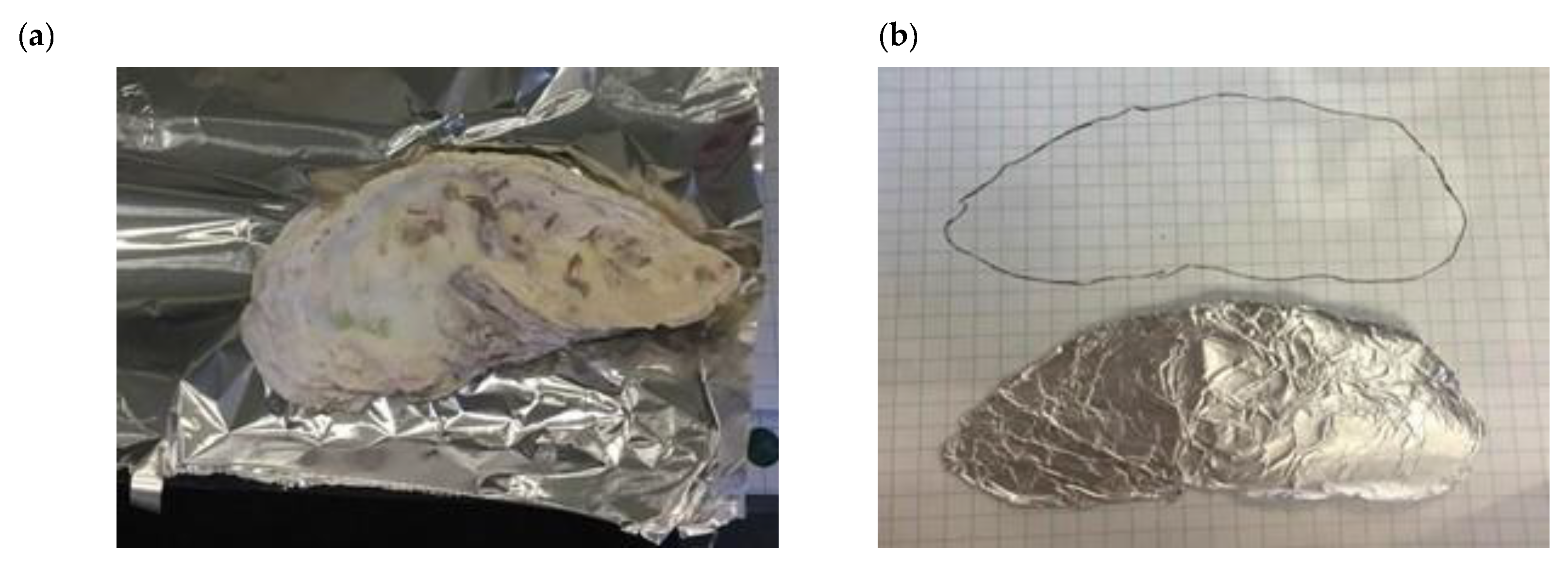
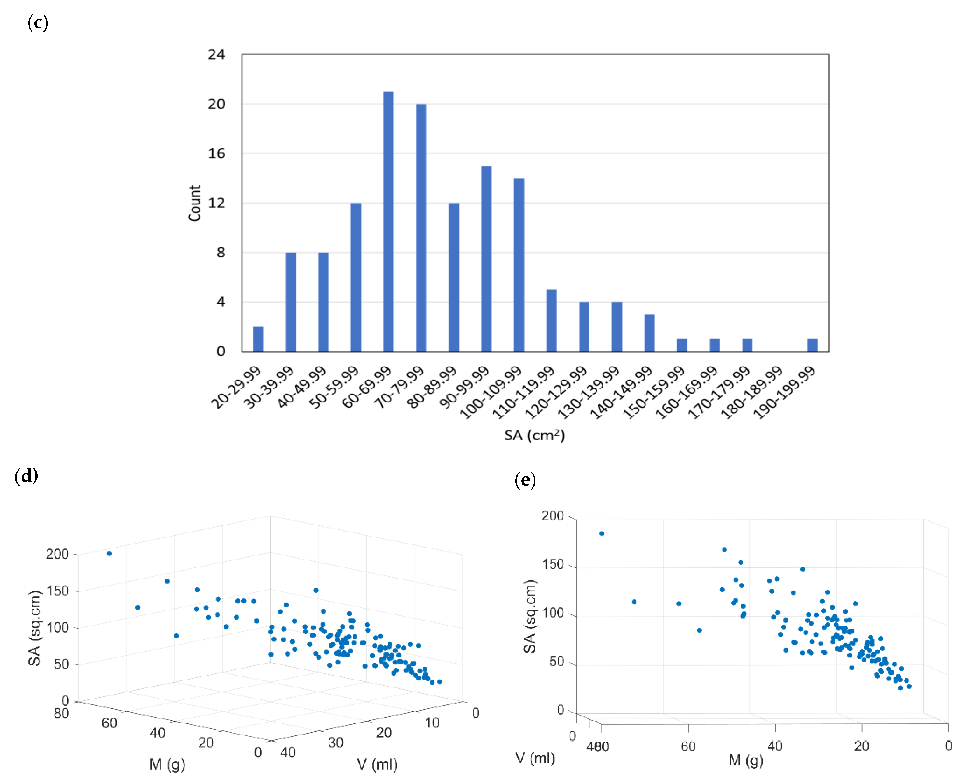
A large quantity of whole and unprocessed oyster shells was obtained from a storage site in Victoria, BC. These shells were originally collected from coastal areas of Victoria and are mainly Fanny Bay oysters from Baynes Sound. In total, 132 shells were obtained for use in this research. Each shell was cleaned carefully with a brush and then air dried. The mass, volume, and SA of each shell was determined before treatment. Because of the shells’ irregular shape, a manual method was developed to measure the SA of each shell as precisely as possible [25]. In this method, sheets of aluminum foil were carefully molded to each side of the oyster shell. The foil mold was cut precisely to the edge of the shell, and then flattened out onto a sheet of paper in order to determine the surface area from a photograph. This is illustrated in Figure 1a,b. The top side of each shell was measured separately from the bottom side (which would be the inside of a closed shell when the oyster was alive in the shell) and all shells were measured and labeled. As shown in Figure 1c, the shells ranged from 26.7 cm2 to 194.6 cm2 in surface area (mean of 82.6 cm2), with mass ranging from 5.8 g to 79.1 g (mean of 23.0 g), and volumes ranging from 3.5 mL to 34 mL (mean of 13.8 mL). Figure 1c shows a histogram of the shell SA and Figure 1d,e are scatter plots of the shell data.
Figure 1d,e show a planar relationship between SA, mass, and volume. To investigate the relationship between SA, mass, and volume for this species of oyster (in order to scale up results from the lab study to the field application), these data were fitted with a function intentionally defined to be dimensionally homogenous with variables M (mass), V (volume), and SA (surface area). In Equation (1a), M has units of grams, V has units of cm3 and SA has units of cm2. Density ρ = M/V has units of g/cm3 and the mean shell density was 1.73 g/cm3 with a standard deviation of 0.59 g/cm3 and a median shell density of 1.64 g/cm3. The proposed equation is
where c and d are constants with units of density (g/cm3) and the constant e has units of grams. The following fitted equation (using Matlab®) produces an R2 of 0.77:
In Equation (1a) the values of c, d, and e should be some portion of the average density of the oyster shells, with e being a reflection of the scatter in Figure 1d,e. Notice that c, d, and e sum to a value similar to the median density. While both the volume and the mass have a bearing on the value of surface area for each oyster shell, for practical reasons, LIDs designed with raw oyster shells would likely be designed with a certain minimum mass of shells. A simple linear regression between SA (cm2) in terms of mass M (g) produces the following expression with an R2 = 0.67:
or
Equation (2) is for practical purposes and suggests a rule of thumb of doubling the amount of mass in grams to get a rough idea of the surface area needed in cm2.
2.2. Individual Experiments for Cu2+, Zn2+, Cd2+, and Cr(VI)
Concentrations of individual contaminants within a stormwater sample will vary widely with the location and event [1]. Thus, a lab-scale experiment targeting each metal individually was conducted. To study the effect of oyster shell SA and metal solution IC on removal efficiency (RE), 4 × 4 individual experiments (including one blank) were proposed for each metal. ET ranged from 1 h, 6 h, 18 h, 36 h, 3 d, 5 d, and 7 d.
Starting with Cu2+, 16 one-liter beakers were prepared with four IC (including a blank with distilled water) and four different SA ranges. After the shells were measured with the method indicated, a comparative analysis amongst the shells divided the 132 shells into four distinct groups such that every shell in a group had a surface area that did not differ by more than 3 cm2 from every other shell in the group. Thus, for all intents and purpose, all shells in a group had roughly the same SA. Given the distribution of 132 shells, the following four differently sized groups naturally arose from the sample: (69 cm2, 85 cm2, 99.5 cm2, and 108 cm2). These separate groups were then used to determine the impacts of SA on efficiency of removing Cu2+ in the initial stages of the experiment. However, initially, the difference in some of the SA groups was too small to see the impact of this variable; thus, one more experiment for Cu2+ with IC = 0.20 ppm with six different SA group sizes ranging from 38 cm2, 121.6 cm2, 223 cm2, 320.8 cm2, 443 cm2, and 550 cm2 was conducted. The initial concentrations for Cu2+ included a blank solution (0 ppm), and three low concentration solutions: 0.23 ppm, 0.93 ppm, 2.79 ppm. During the experiment, the beakers were covered with a piece of plastic wrap to prevent water from evaporating. Four parameters, including pH, temperature, electric conductivity (EC) and concentration were monitored for each ET. The values of pH, temperature and EC were tested with a YSI Sonde EXO2 six parameter probe with accuracies of ±0.2 °C on temperature, ±0.1 of pH and ±1% of reading on EC. A LaMotte Smart Spectro 2 Spectrophotometer was used to measure concentrations with Diphenylcarbohydrazide reagent for Cr(VI); Bicinchoninic Acid reagent for Cu2+; 1-(2-pyridylazo)-2-naphthol reagent for Cd2+, and Zincon reagent for Zn2+. Although initial concentrations were prepared based on molar calculations to achieve a desired IC, when measured with the spectrophotometer, deviations from the expected values existed. Thus, the concentration recorded for IC was the one produced by the spectrophotometer and not that determined from molar calculations.
Similarly, for Zn2+, Cr(VI) and Cd2+, 3 × 3 individual experiments were devised. For Zn2+, 1 ppm, 0.5 ppm, and 0.2 ppm IC were tested with 35 cm2, 154 cm2 and 303 cm2 sized shells (same ET range as Cu2+). For Cr(VI) the same concentrations were tested with 37.8 cm2, 151 cm2, and 300.5 cm2 and similarly for Cd2+ but with shell sizes of 43 cm2, 152.8 cm2, and 300 cm2. Again, the initial concentrations recorded by the spectrophotometer were used in the analysis.
The removal efficiency (RE) in this work was calculated as
where Co is the initial concentration (mg/L) and C(t) is the concentration at time t (h) [1,26]. In addition, because several processes in wastewater treatment follow a first order kinetic, modelling was conducted to determine if the removal process for each of these metals by oyster shells followed a first order kinetic model. The general model of a first order kinetic [26] is:
where k is the reaction rate in units of h−1. In addition, to investigate the possibility of a higher than first order reaction, the following was used:
where a second order reaction is being explored.
2.3. Mid-Scale Experiment
In wastewater treatment, hydraulic retention time (HRT) is an important parameter related to inflow rate and reactor volume. HRT in the field of environmental hydraulics [26] is a parameter in completely mixed flow reactors (CMFR) or plug flow reactors—two models used to understand the transport and retention of pollutants in large water bodies like lakes. In the implementation of whole oyster shells for use in the field to treat stormwater, exposure time (ET), which is related to HRT, needs consideration as the type of exposure seen in wastewater treatment is not the kind of exposure expected in LID systems. To treat stormwater with a biosorption material, the LID must be designed with a minimum HRT, noting that stormwater is intermittent. In large scale systems like LIDs, ET is intimately connected with HRT but generally,
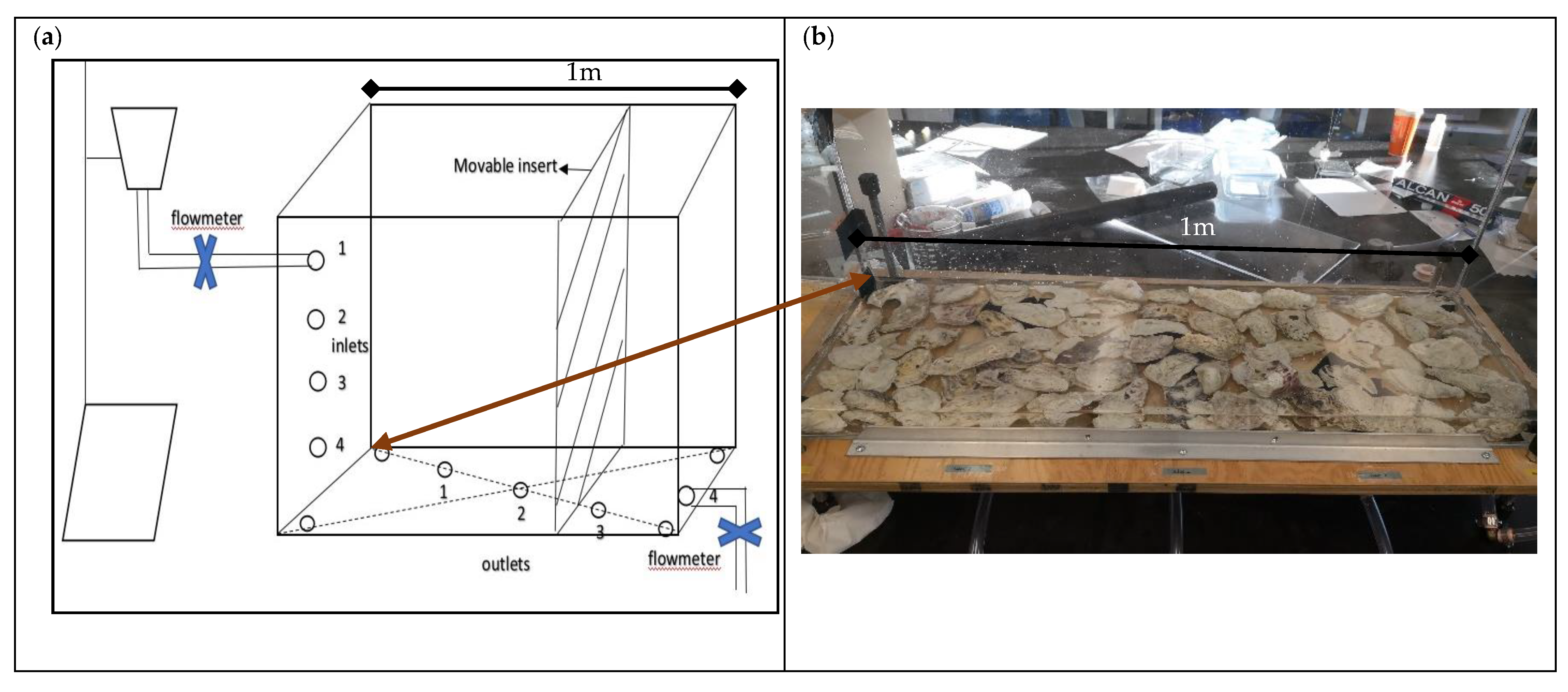
where Ve is the effective volume of the reactor or container (m3) and Q is the effective outflow rate (m3/h) giving an HRT in hours [26]. To explore a larger scale application above the lab scale, and which could allow the exploration of HRT values that may exist in actual LID systems, a mid-scale device was designed and fabricated to mimic real conditions as closely as possible. This device was composed of five plexiglass pieces and an additional piece that is movable inside of tank to change the tank volume. The base is on adjustable pedals allowing the tank to achieve a desired slope to permit drainage by gravity. The overall dimensions are approximately 1 m length × 0.6 m height × 0.3 m width. The design of the mid-scale tank is shown in Figure 2.
The mid-scale experiment differs from the lab-scale beaker experiments in that the latter only uses standing water. The mid-scale experiment is intended to mimic runoff to an urban infrastructure with an inflow and outflow. The exposure time, or HRT would all be related to the elapsed time from the start of the storm which enters the tank in 20 min increments. The inflow combines and mixes with treated water exposed to the shells, and 60 mL is extracted every 20 min to mimic outflow. The outflow would then be a mixture of new and treated inflow. It is difficult to know the extent to which the inflow is in contact with the shells and what portion remains untreated, but some mixing is assumed, as it would be in real-world LID applications.
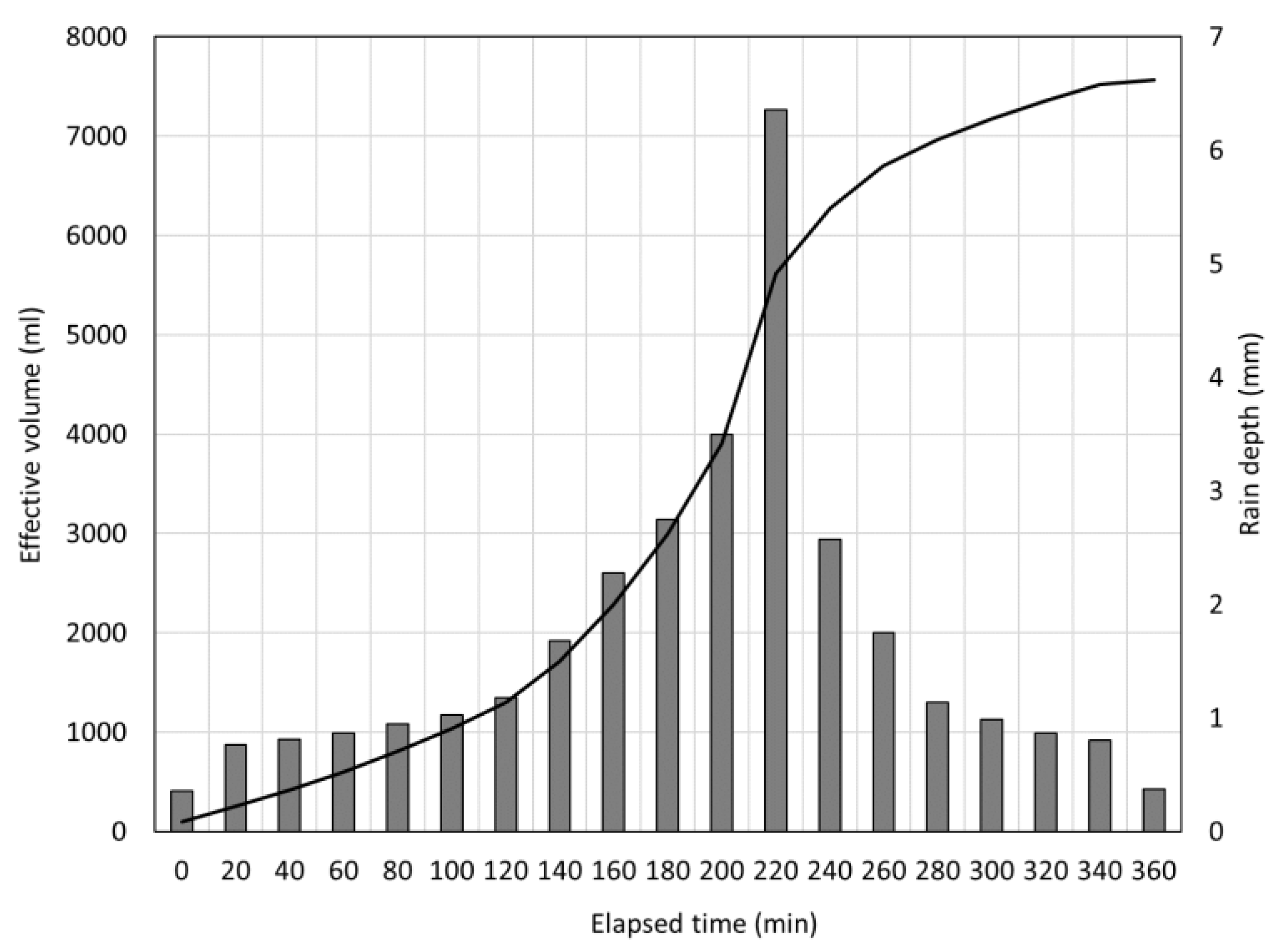
The mid-scale experiment was conducted according to the 6-h Duration Design Storm from the District of Saanich (in Victoria, British Columbia, Canada) Stormwater Modeling Standards [27] but 20 min increments were used instead of 10 min increments (see Figure 3). The inflow volume every twenty minutes was calculated based on rain depth and the bottom surface area of the tank (2787 cm2). Thus, if the initial inflow (rain depth) is 0.36 mm, this produces 0.1 L when multiplied by 2787 cm2 and the first flush would be 100 mL. The specific data are shown in Figure 3. A 10.465 L sample solution was prepared mixed and confirmed by testing with 0.5 mg/L Zn2+, 0.55 mg/L of Cd2+, 0.33 mg/L of Cr(VI), and 0.62 mg/L Cu2+ in one solution. A layer of shells was put on the bottom of tank with a total surface area of 9437 cm2, mass of 2660 g and volume of 1600 mL shown in Figure 2b. The concentrations of Zn2+, Cu2+, and Cr(VI) were tested with the spectrophotometer, but a separate Cd2+ test from LaMotte was used to test Cd2+ with 0.1 ppm accuracy. When the experiment began, every corresponding volume of water was poured into the water jar and flowed into the tank from the inlet continuously for twenty minutes. At every 20 min increment, 60 mL from the furthest outlet was collected and tested for various parameters. Outflow was monitored again at 1, 4, and 7 days, to see if anymore contact time could increase removal. Therefore, in the tank experiment, elapsed time is not the same as elapsed time in the beaker experiment (in which elapsed time is also equal to contact time).
Considering the formula of HRT in Equation (6) for the system, the volume Ve is divided by either inflow rate or by the outflow rate (Q in Equation (6)). For HRT calculations in wastewater treatment, Q is the inflow rate which varies and thus, Ve also varies because it is a function of Q. Therefore, HRT was calculated every twenty minutes, and the volume of water at that time would be considered as Ve and Q is the inflow rate at that twenty minutes. For a CMFR or PFR (plug flow reactor [26]) system representing large water bodies and LIDs, Q is the outflow rate, which is 60 mL/20 min equal to a constant 3 mL/min. Ve is the cumulative volume minus cumulative outflow.
The equation governing both a CFMR and a PFR system is
where m is the mass of the pollutant in the system, is the mass flux in, is the mass flux out and is the mass rate of change solely due to the reaction. For a first order decay reaction,
and Ve is that of Equation (6), k is that in Equation (4) and C is the concentration of the pollutant in the tank at time t.
Given the physical size of the tank, and the way inflow and outflow were generated, in the early stages of the storm, the system is assumed to be most represented by a non-steady state CFMR with first-order decay. This results in the following expressions in their differential and integral forms:
where Qin is the inflow rate, Cin is the concentration in the inflow, Qout is the outflow rate, and Cout is the centration of the pollutant in the outflow. Given the inflow follows the design storm, the inflow concentration and the outflow concentration are both fixed, and assuming that the concentration C in the tank at any time t is equal to the concentration in the outflow Cout at that time t, and converting to discrete form, Equation (9b) reduces to
where t = nΔt, Δt is the time increment of 20 min (or 0.333 h) and n = 1, …, N where NΔt marks the end of the experiment. A simple spreadsheet can be used to compute k as all parameters are either known or observed. The parameters Ve and Qin at every time t are effectively given in Figure 3 and Cout is measured at the outflow.
3. Results and Discussion
3.1. Lab Scale Experiments on Individual Metals
3.1.1. Influence of IC on Removal Efficiency of Cu2+ over Varying ET
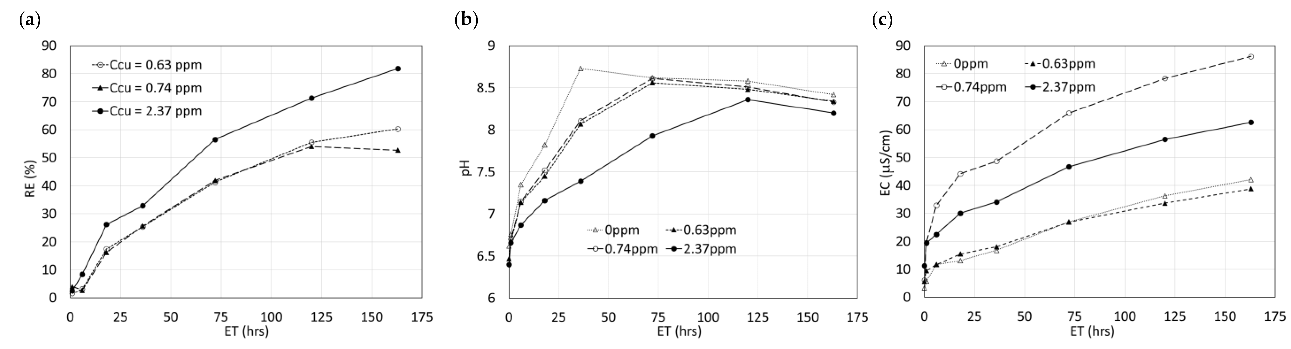
Figure 4a illustrates the relationship between removal efficiency RE and ET for varying IC for the largest shell in this experiment (108.05 cm2). Because the curves for the different SA values varied only marginally for each IC, only the curve for the largest SA is shown. Figure 4b,c show the changes in pH and EC, respectively. Temperature was observed to fluctuate between 18 °C to 21 °C throughout the experiment (with a standard deviation of approximately 1.2 °C). This was not considered an influencing factor in the results.
Figure 4a not surprisingly shows higher removal efficiencies for the highest IC, which is similar to results seen in Liu et al. [15]. The two lower concentrations that were originally designed to have a greater difference in value were measured by the spectrophotometer as 0.63 ppm and 0.74 ppm. Figure 4b shows that there is desorption of calcium ions into the water as the 0 ppm concentration solution increases the fastest of all three solutions and the highest IC solution has the lowest ranges in pH. Interestingly, Figure 4c, which illustrates the electrical conductivity measurements over ET, does not show the same tendencies with IC as it does with pH in Figure 4b. As both are measures of the number of ions in the solution, the results should be roughly similar in trends. The 2.37 ppm solution produces a higher electrical conductivity than does the 0 ppm and 0.63 ppm solutions, but the 0.74 ppm solution produces the highest electrical conductivity measurements. This may possibly suggest that this particular data set may be anomalous with respect to the processes involved, although the authors could not definitively point to a reason for this anomaly given all the data.
3.1.2. Influence of SA on Removal Efficiency of Cu2+ over Varying ET
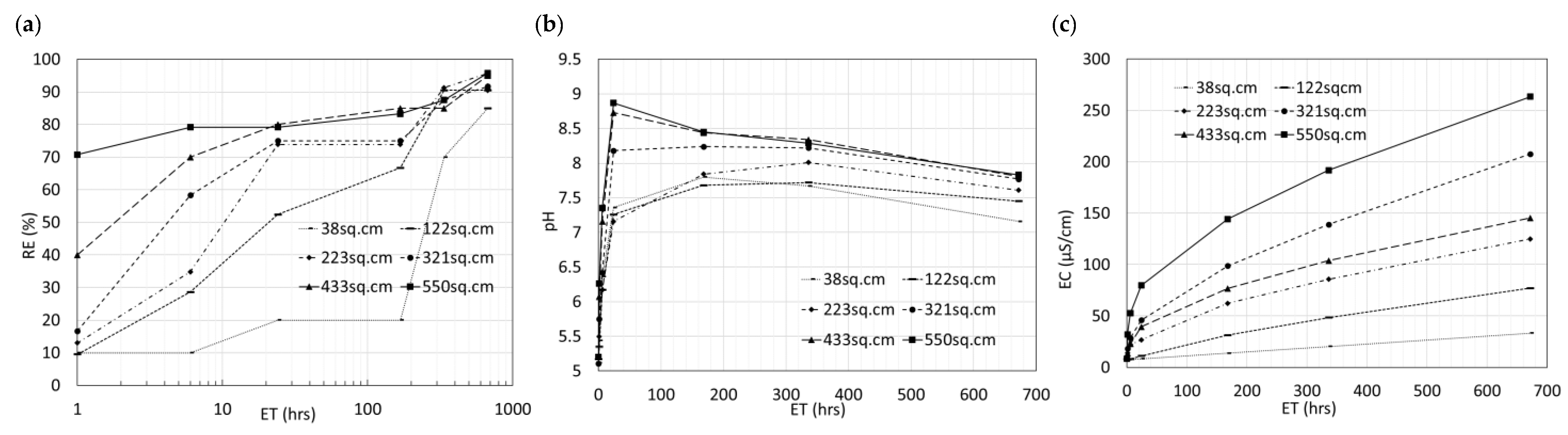
Figure 5a shows the results of the Cu2+ experiment that used six SA groups and an initial concentration of 0.20 ppm. The relationship between RE and ET is clear from Figure 5 such that the beaker with the larger surface area reaches the same RE quicker than that with smaller SA values. As can be seen from Figure 5, shells with different surface areas (average size shown in the legend) can reach over 85% after 28 days; however, when ET is 1 h, the beaker with the largest SA of 550 cm2 already showed a removal efficiency of 71%, but the shell with a small SA of 38 cm2 only removed 10% of the metal ions in solution. Moreover, the removal rate of the smallest three surface areas shows very large differences, but when SA is between 223 cm2 and 550 cm2, the difference in removal efficiency after 24 h is quite small. Overall, the most reactive period is in the first 24 h and after that, removal efficiency for SA over 223 cm2 shows similar RE trends. This is similar to observations in the literature [19]. Figure 5b shows the increase in pH is also related to SA. The initial pH values were the same for all solutions, but after placing shells into the beakers, pH increased and the solution with more SA present in the beaker increased at a higher rate as compared to smaller SA for the same ET. This phenomenon matches the concentration trends. The pH fluctuation during the rapid reaction period is also dramatic. Similarly, in Figure 5c, electric conductivity also increases over longer ET and shows a strongly positive relationship with SA (also seen in the literature [19]).
Given the trends observed in Figure 5, and to further explore the role of SA in removal efficiency given contact time, power relationships were fitted to every curve shown in Figure 5a using Microsoft Excel® in the following form:
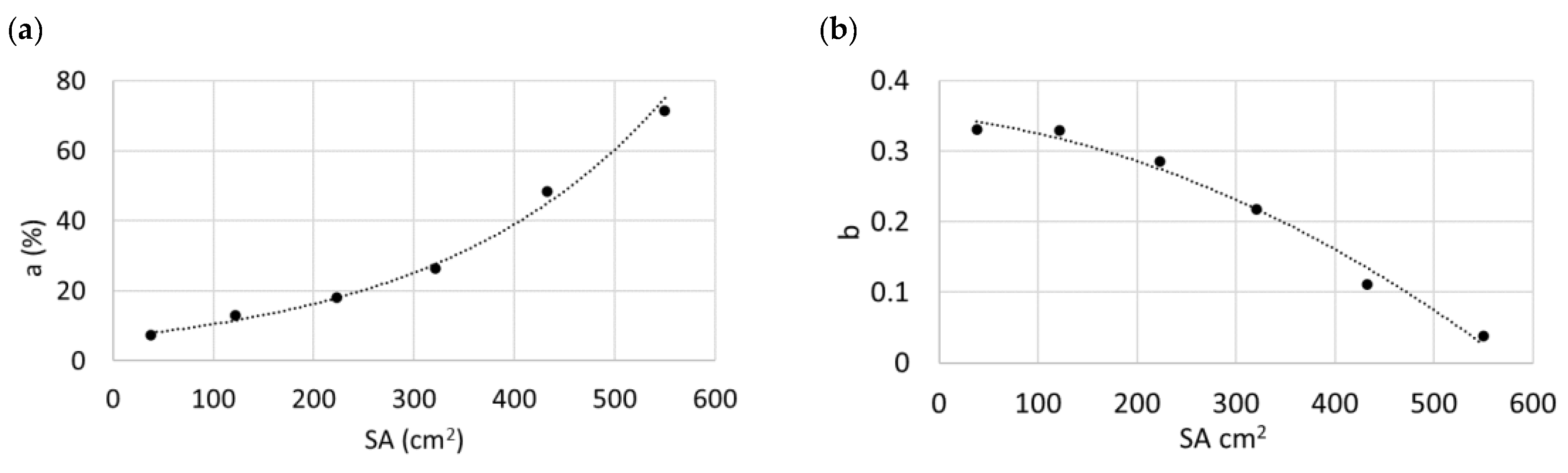
This relationship produced an R2 ranging from 0.74 to 0.92 across the curves and the coefficients a and b were seen to show a trend as a function of SA. Thus, the coefficients a and b of Equation (11) were plotted versus SA and are shown in Figure 6a,b, respectively. The best fit functions for each curve in Figure 6 were shown to be the following:
Coefficient a in Equation (11) technically represents the basic or minimal rate of metal removal without the use of oysters (SA is near zero). However, this is not a true lower limit because if SA = 0, technically, there can be no removal efficiency and is merely an artifact of the accuracy limits of the experiment. Parameter b is a modifier that is a function of the units involved to describe SA (cm2) and removal efficiency (%). While the absolute values of both a and b are related to the units used to create the functions, the form in which a and b relate to SA would involve characteristics of the whole, unprocessed oyster material that lend to the ion-exchange process, and therefore dependent on the material type. Figure 6 clearly shows that the exposure time required to remove a certain percentage of metals decreases with the amount of SA available in a non-linear manner. The higher the SA, the factor coefficient a exponentially becomes closer to 100% for any given ET, while the exponent coefficient b gets closer to zero following a second order polynomial. The fact that a is exponentially related to SA shows that even minimal differences in SA can have significant impacts on removal and speaks to the strength of the ion exchange process afforded by unprocessed, whole oysters shells. According to Equations (12) and (13), as the total shell surface area exceeds 610 cm2, parameter a reaches near 100% while b becomes nearly zero and, thus, effectively removing the exposure time as a factor in the equation. This suggests that providing these levels of oyster surface area, and therefore (according to Equation (5)) enough oyster mass to exceed 1.5 kg in total mass, in a beaker like setting (such as at the bottom of a catch basin), then one could effectively remove Cu2+ in the very early stages of a storm.
3.1.3. Influence of IC and SA on Removal Efficiency of Zn2+, Cr(VI), Cd2+ over Varying ET
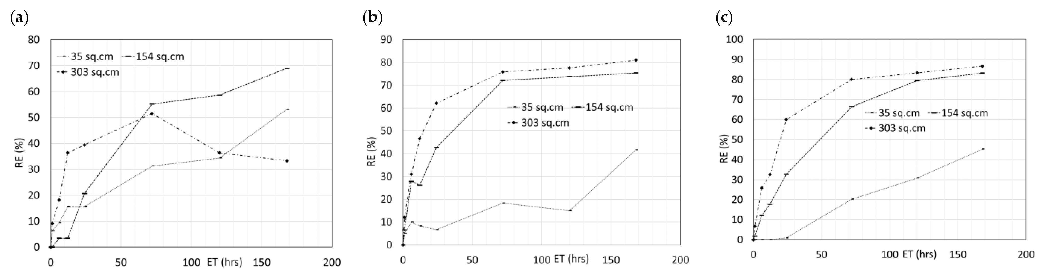
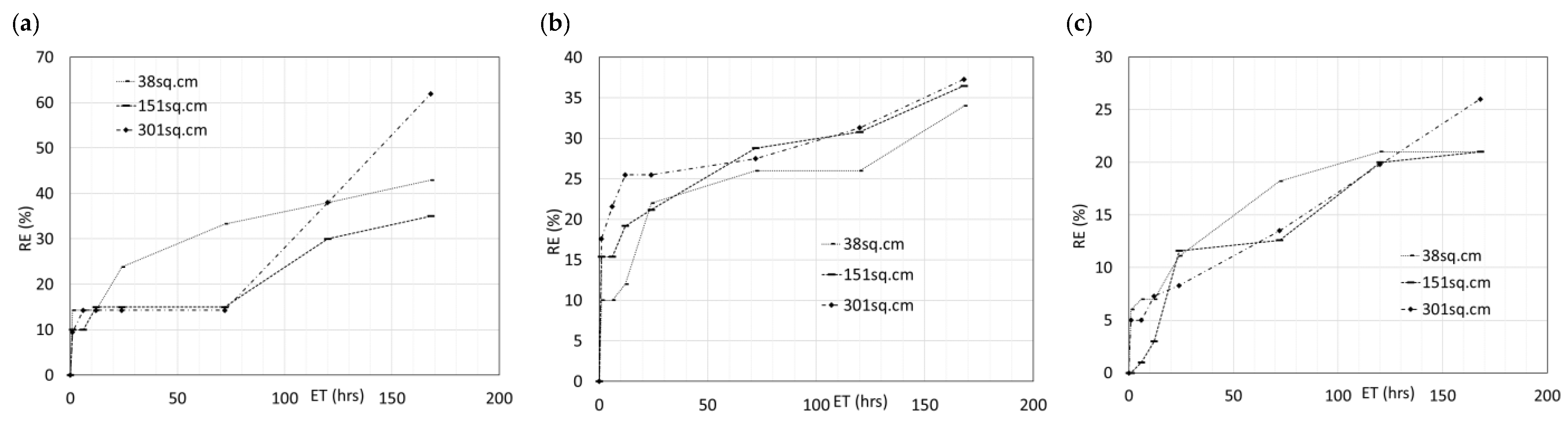
For Zn2+, Cr(VI), and Cd2+, a 3 × 3 factorial design experiment was conducted for each metal such that three ICs were crossed with three SA group sizes. All initial concentrations were devised as 0.2, 0.5, and 1 mg/L, but again, the recorded initial concentration was that provided by the spectrophotometer. Temperature ranged from 18 to 24 °C in all the experiments. In terms of EC, the contact time was generally, positively related to EC and larger SA tended to produce higher EC values as was seen for Cu2+. For Zn2+, the largest SA always had the highest EC. For Cd2+, EC data were similar for larger SA for up to differences in SA of 150 cm2. For Cr(VI), EC was shown to have a stable increase, but the results were inconsistent in terms of larger SA producing higher EC.
The absorption ability of the same amount of shells tended to have a higher removal efficiency with increased initial concentration. For Zn2+, the shells of 154 cm2 showed 69%, 75%, and 83% when IC is 0.3, 0.6, and 1.07 ppm, respectively. For Cd2+, the effect of initial concentration did not seem to be important. When IC increased from 0.26 ppm to 0.95 ppm, removal efficiency of the maximum shells reached close to 90%. There was little difference in removal efficiency for different initial concentrations. Moreover, the difference in the two largest SAs on removal efficiency is small for a longer contact time for different IC values. A larger SA should react with metal ions faster over the same time and the removal efficiency did show a strong relationship with exposure time. A negative relationship between RE and IC was found for Cr(VI) removal, which is unlike the other metals (RE positively related to IC). It was observed that 300 cm2 of shells can remove over 60% in solution with IC of 0.2 ppm, 37% in solution with IC of 0.5 ppm and 26% in that of 1 ppm. This observation for Cr(VI) is consistent with the literature [14,22], which generally showed poor removals of Cr(VI) by oyster shells.
Figure 7 shows the RE produced for the Zn2+ solutions. The higher SA produced higher removals of Zn2+ and this was nearly consistent across all IC values. The one anomalous trend was seen in the smallest IC and the largest SA declining in removal efficiency after 80 h or 3 days; also, maximum removal efficiencies in this experiment never reached 90%.
Figure 8 shows the removal efficiencies of Cr(VI) ions for three IC values. This metal showed a much lower efficiency compared to other metals which is most likely because of the ion radius difference [23]. While the larger shells achieved the highest removal efficiency, the effect of SA is not apparent in higher IC solutions.
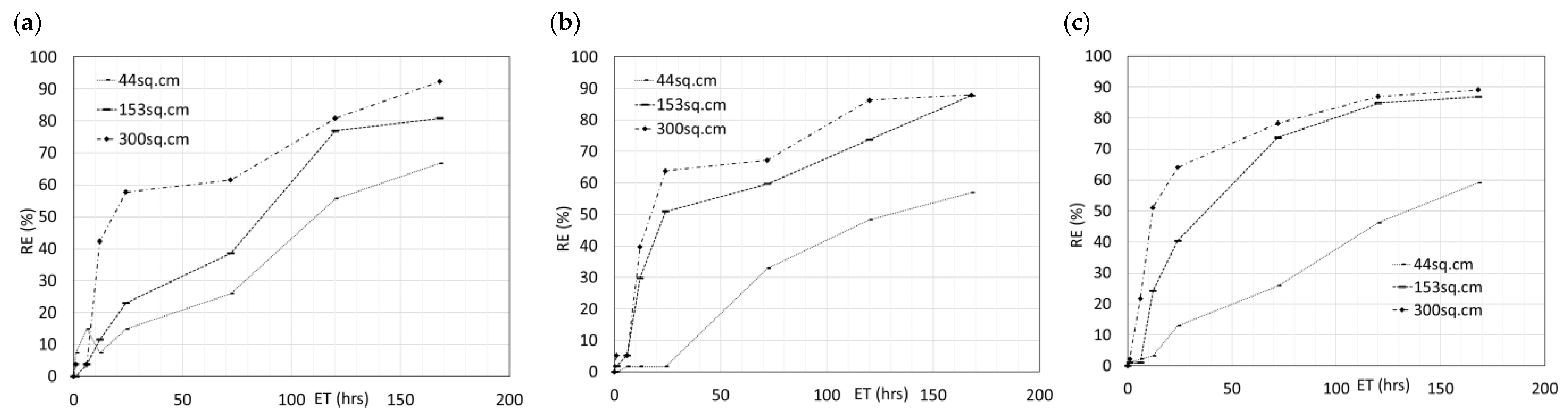
Figure 9 shows that the removal efficiency of Cd2+ also had a strong relationship with exposure time. At seven days, the RE of shells from the smallest SA to the largest SA was 67%, 81%, and 92% for IC of 0.26 ppm; 57%, 88%, and 88% for IC of 0.58 ppm; and 59%, 87%, and 89% for IC of 0.95 ppm. As noted, for Cd2+, the effect of initial concentration did not seem to be important. Moreover, the difference found with the two largest SAs on removal efficiency is small for longer contact times. For example, when IC is 0.58 ppm and 0.95 ppm, and SA is 152.8 cm2 and 300 cm2, the removal efficiency was almost the same after seven days. According to measured pH, the reaction was active in the first day, with a pH ranging from 5.7 to almost 9, with an average removal of around 60% for all initial concentrations. The pH for all solutions were stable at around 8 after seven days, compared to an initial value of 5.7. Electric conductivity data were similar for larger SA values, even with a difference in SA of 150 cm2. In general, the data suggest that although a positive relationship between SA and RE exists, it does not suggest that having more shells is necessarily better after a certain threshold of SA. Above a certain amount of shells, the difference in SA can be negligible, which also matches the results found in the Cu2+ experiment. The variability in results for Cd2+ is consistent with the variability found in the literature [14,19,20] in which Cd2+ absorption to be highly affected by pH and were typically low.
3.2. Mid-Scale Experimental Results
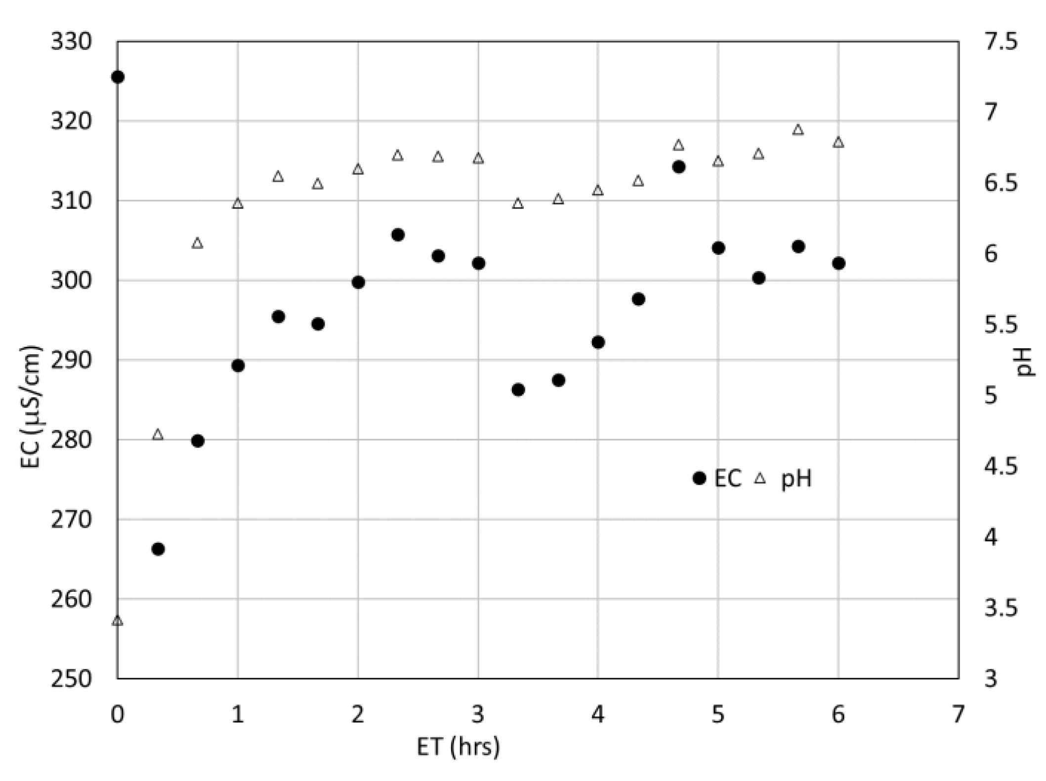
Figure 10 shows the pH and EC levels over the elapsed time in the mid-scale experiment. The temperature ranged from 19 to 22 °C. As the figure shows, the mixture solution has a low pH of 3.5 initially and increased quickly in the first 40 min to about 6, then fluctuated between 6 and 7 for the rest of the experiment. The EC varied in a similar manner to the pH curve, stabilizing somewhat at approximately 314 μS/cm.
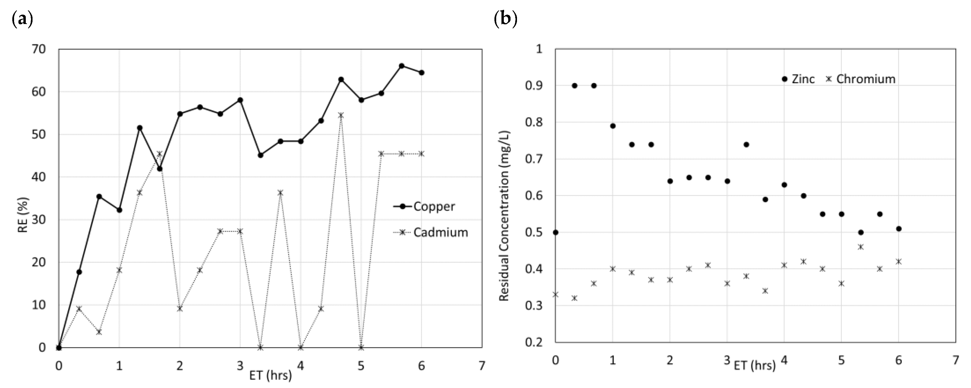
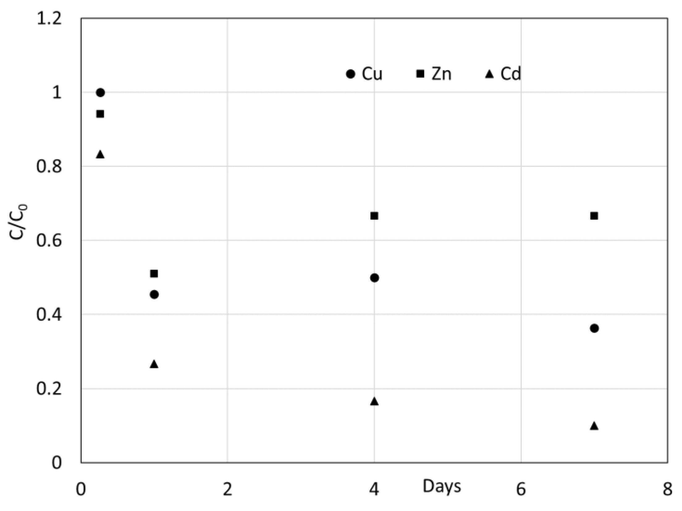
Figure 11 shows the removal efficiencies for each of the metal ions. In the 6-h storm, Cu2+ was treated to a relatively high RE compared to other metals, proving that oyster shells are effective in removing Cu2+. At 80 min, RE is over 50% even with continuous inflow and with only one day of contact time, RE can reach over 80%. Although longer times can improve RE slightly, given practical considerations and the issue with pH, 24 h should be the best reaction time for Cu2+. The pH increased gradually after the six-hour storm from 6.8 to 7.9 from 6 h and 20 min to 7 days. This also matches the lab experiment for Cu2+, where RE was around 80% in one day for the maximum and second largest shells (Figure 11a).
Zinc metal ions and Cr(VI) (Figure 11b) did not show any removal in six hours of inflow; inversely, their concentrations tended to increase. Especially for Zn2+, the concentration increased from 0.5 ppm initially to 0.9 ppm at only twenty minutes. This phenomenon was not expected but rational: the mechanism of oyster shells for absorbing metal ions is based on the chemical reaction between ions and calcium. However, the actual mechanism of absorption would be much more complicated and would include physical and chemical adsorption. Although this paper does not focus on exploring these mechanisms individually, physical adsorption should exist. Note that the shells used in the mid-scale experiment had previously been used in the individual experiments. Therefore, the increasing concentration of Cr(VI) and Zn2+ is likely because of inflow flushing over the ions that were physically fixed on the surface of the shells. The authors found that after an initial sharp increase in Zn2+, the shells removed Zn2+ gradually, to the same final concentration at six hours. Samples were taken at later times to test the concentration of Zn2+ at one day. Zinc ions were reduced to 0.26 ppm, which is basically 50% RE. However, a slight increase of concentration of Zn2+ can be seen with longer times than one day which is probably because of physical desorption of Zn2+ ions again. It is believed that chemical adsorption is more stable than physical desorption but would take some time to realize. These observations for Cr(VI) and Zn2+ are also seen in the literature [14,15,19,22].
Whole oyster shells were proven to be somewhat effective in removing Cr(VI) in the lab-scale experiment, but in the mid-scale tank, there was little to no removal as seen in Figure 11b. This is likely because of competition among metal ions.
Cadmium metal ion concentrations (Figure 11a) in this portion of the experiment were tested with a Cd2+ concentration kit from LaMotte with code number 7839-02 and the value was given based on comparison to a color bar as part of the kit. Despite the lower precision than the spectrophotometer, a rough tendency can be seen in the figure. RE of Cd2+ varied according to inflow amount and was finally stable at around 45% with low runoff. However, an RE of 85% can be reached in one day of contact time, and RE also grew over time to over 90% (figure not shown). This means Cd2+ ions require larger contact times with the shells to reach high removal efficiencies. For Cd2+, one day is still the best time for removal. Table 1 shows the residual concentrations, EC, and pH for the four metal ions up to 7 days after the experiment was initiated.
3.3. First and Second Order Kinetic Modelling
For modeling the adsorption kinetics, the data obtained in the individual experiments with different initial concentrations but with the same size shell group were combined. The concentration C(t) at each time t was divided by IC (Co) in order to group the data to determine the rate k in Equations (4) and (5). Then the exponential functional form shown in Equation (4b) was fit to the data of C/Co versus t to determine k in Equation (4). To determine the possibility of a second order relationship, Equation (5a) was rearranged and a plot of 1/C − 1/Co versus time t with a straight-line fit was computed.
3.3.1. Modelling Individual Metal Ion Concentrations with Initial Cu2+ Results
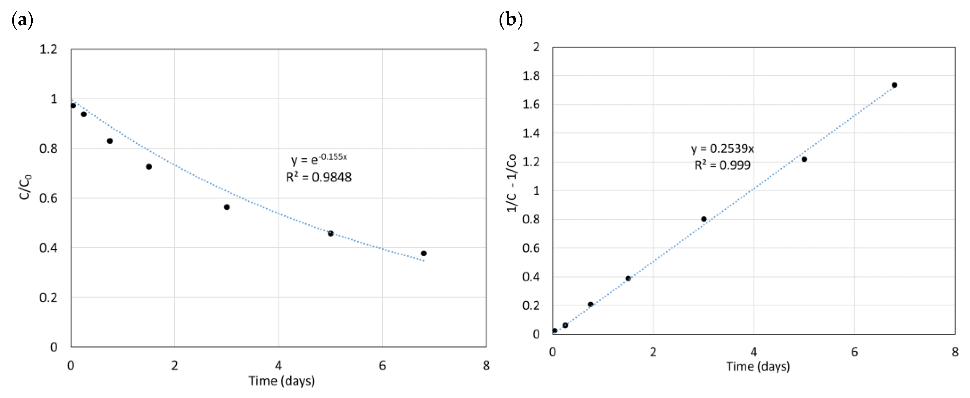
For the first set of Cu2+ individual experiments in which variations in SA did not make a large difference in the outcomes, the average of all the concentrations for all SA values was calculated and used for 1st and 2nd order kinetic modelling. Figure 12a shows all the averaged data and the best fit, first order curve for C/Co. The best fit line produced an R2 of 0.96 and k = 0.155 days−1. Figure 12b shows the straight line fit to the data plotted to indicate a second order kinetic. Here the fit is better with an R of 0.99 with a k value of 0.254 days−1. While the fit for the 2nd order kinetic model is marginally better, it suggests a decay rate that is 1.6 times greater than that for the 1st order kinetic, which is not surprising with the mathematical models used here. However, there is not enough evidence to suggest that one is more representative of the process than the other.
3.3.2. Modelling Individual Metal Ion Concentrations with Second Set of Cu2+ Results
The second set of Cu2+ experiments were affected by SA so averaging across SA was not considered reasonable. In this case, all the data could not be combined and so the first and second order kinetic parameters were determined for each SA value and are shown in Table 2 and Table 3, respectively. In Table 2, both Equation (4b) and the equation of −ln(C/Co) = e + kt were tested. In the latter case, e is the error deviation from a purely exponential decay rate. For Table 3, only Equation (5) was tested.
The kinetics model is used for explaining the adsorption process, but in this work, it is used to estimate the reaction rate. In the second set of Cu2+ experiments, the k values with no error term seen in Table 2 are similar for all but the smallest SA. The coefficient of determination however degrades to zero as SA gets larger. When an error term is given, the rate factors k are again similar but the error term grows with increase in SA. Table 3, which uses a second order reaction, provides values with no error term and all the R2 values are consistently high and are similar for half of the SA groups. If ignoring SA = 38 cm2, then the k factor is somewhere around 2/day to 3/day. Given the desire to maintain a minimum surface area/mass of oyster shells in the LID, the data associated with the higher values of SA should be given greater consideration. Thus, the data in the second set of Cu2+ experiments and with SA values of either 433 or 550 cm2, are those likely providing the most reasonable estimate of reaction rate in an actual application in the field.
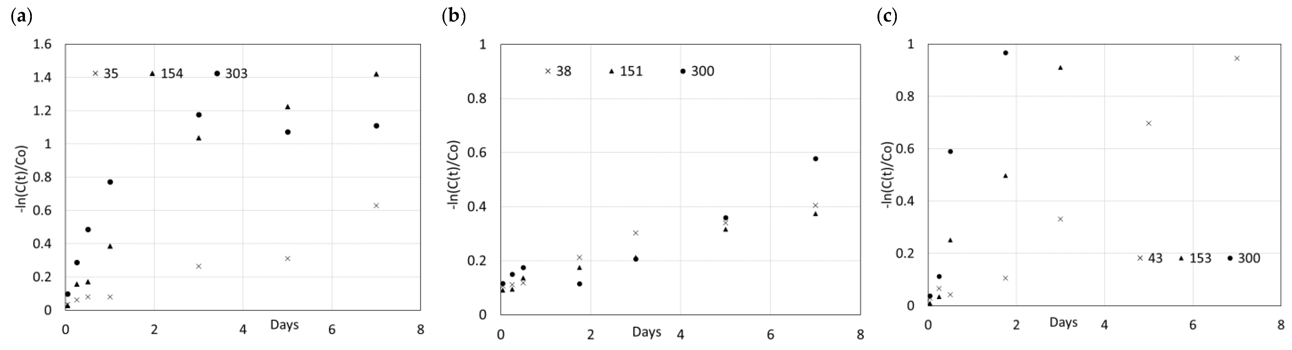
The first order kinetic model was also applied to Zn2+, Cr(VI), and Cd2+ in which Equation (4) was used in Figure 13 to determine the reaction rates for each metal. For every shell size, the average of the three results for varying IC was taken and plotted in Figure 13. Table 4 shows the results of the best fit line representing Equation (4). The results show that there are fair to good removal of all three of these metals in as little as one day. Efficacy for removal was generally highest for the largest shell size and of the three metals, oyster shells seemed to be the least efficient for Cr(VI) removal. First order kinetic modelling is a reasonable representation of the reaction rate for all three metals. If the highest shell surface area is considered, the reaction rate for Zn2+ and Cd2+ are of similar orders of magnitude and around 0.2/day to 0.4/day. This is also similar to that of the first order kinetic reaction rate k for Cu2+. Hexavalent chromium, which was not removed by the oyster shells with a high efficacy, showed a first order reaction rate that was an order of magnitude smaller for the largest oyster shell group. Again, looking across Cd2+, the reaction rate increased with increasing shell area and for Zn2+, this was also suggested although not as evident due to the low coefficient of determination for the SA = 300 cm2 group with no error term.
3.4. Modelling Metal Ion Concentrations in the Mid-Scale Environment
Given the results of Figure 10 and Figure 11, it is evident that ion exchange in the tank, which contains all of the metals in solution (as opposed to that of the lab-scale experiments in which individual elements were tested), is favoring Cu2+ absorption, then Zn2+ absorption (similar to what was observed in [20]), leaching of Cr(VI), and absorption and leaching of Cd2+ throughout the experiment. Copper ions and Cd2+ showed some removal while Zn2+ showed an initial jump and then a gradual decline in concentration. Hexavalent chromium was not effectively removed in the mid-scale experiment and this is consistent with the results in the literature (potentially due to the moderate levels of pH [22]).
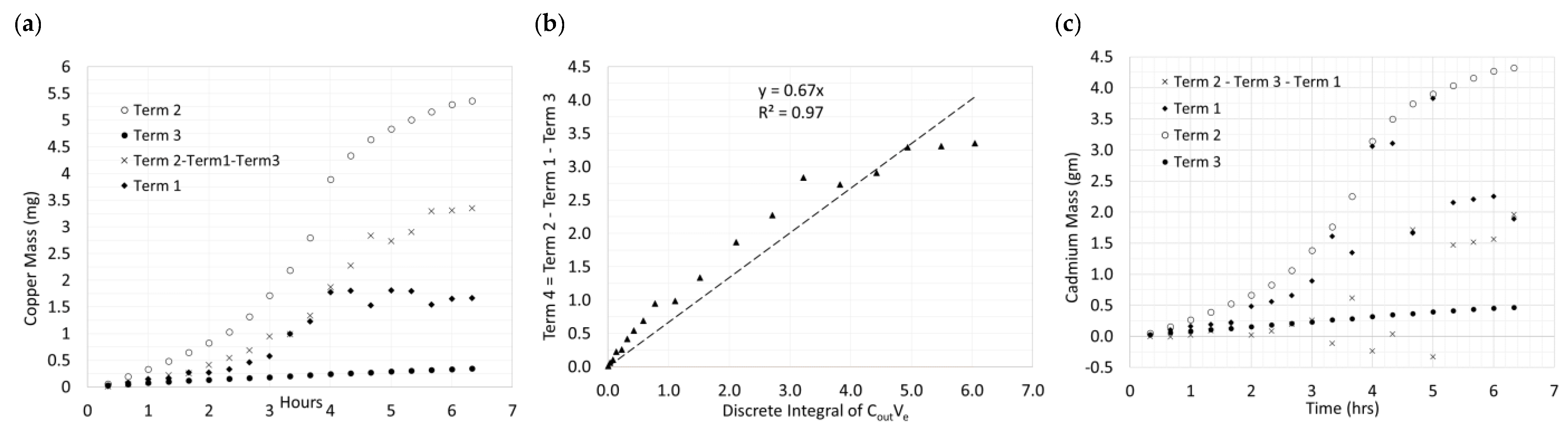
Modelling the concentration of each metal in the tank as indicated by Equation (10) may produce single k values for Cu2+ and Zn2+, but the reaction term in Equation (7) would oscillate between negative and positive values and could not be pulled out of the integral in Equation (9b), as it would vary over time. Thus, for this study, Equation (10) was only used on Cu2+ and Cd2+ for the “storm” duration, and on Zn2+ after the first 20 min (in which the Zn2+ concentration in the outflow increased from Cin = 0.5 mg/l to 0.9 mg/L). Every term in Equation (10) was computed for each time step and plotted separately in Figure 14 for Cu2+ and Cd2+, and Figure 15 for Zn2+.
From Equation (10):
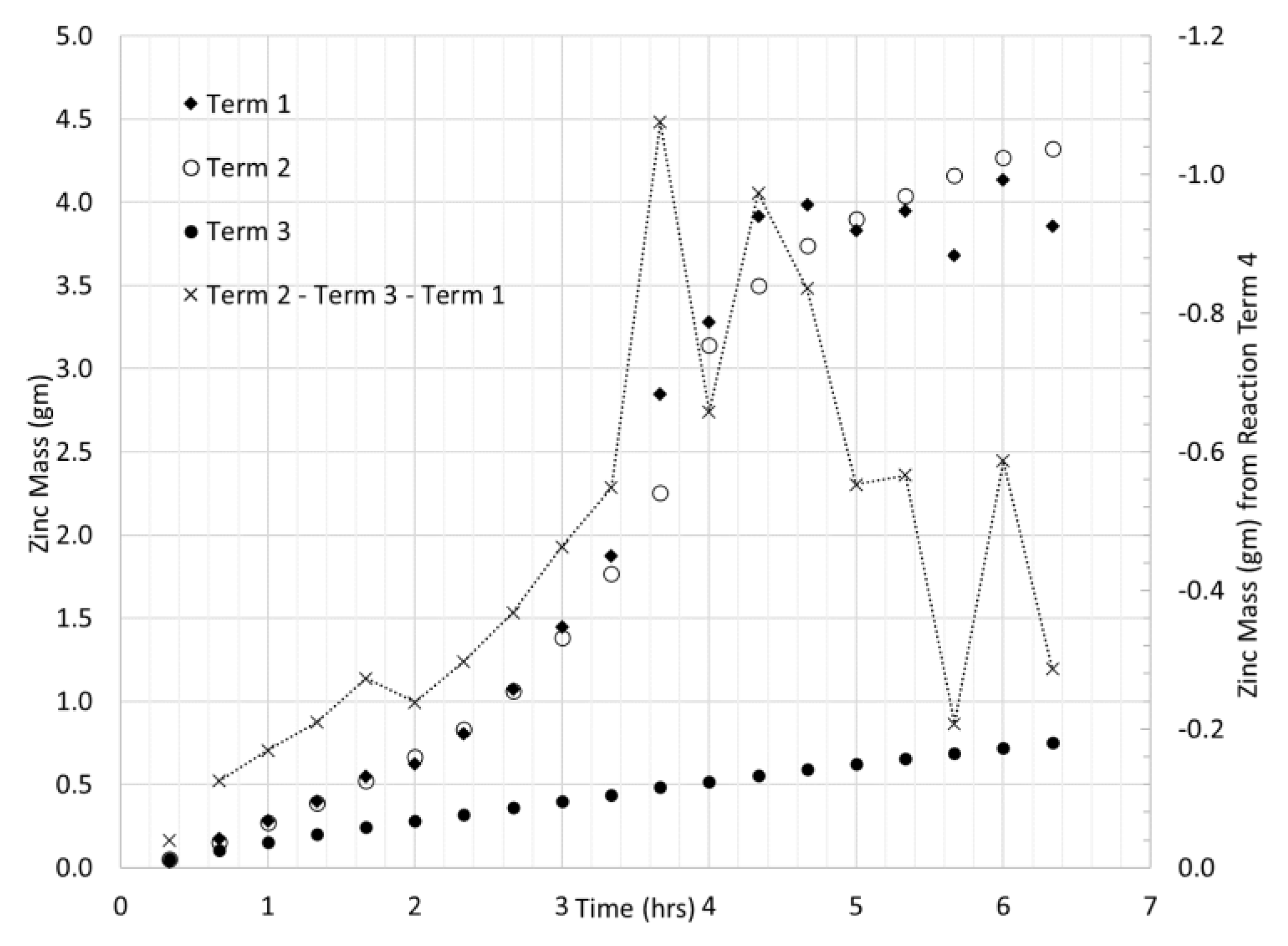
Terms 1, 2, and 3 are computed from known inputs and observed outputs. Term 4 is computed as equal to (Term 2 − Term 3 − Term 1) and plotted in Figure 14a for Cu2+ and 14c for Cd2+. Note that for Equation (10) to be applied, the time step is constant and here equal to 20 min. Thus, Figure 14 is only shown for the first 7 h in which the variables in Equation (10) were measured every 20 min. While k may be suggested from the individual lab-scale experiments, it is worthwhile to look at Term 4, and each component of Term 4 separately. Figure 14b therefore, is a plot of Term 4 as computed above, vs. for the first 7 h for Cu2+. Theoretically, this should produce a best fit line which, is also shown in Figure 14b as well. Figure 15 shows these same modelling results for Zn2+.
Figure 14b illustrates that at least for Cu2+, it is highly probable that Equation (10) captures the mechanisms for Cu2+ concentration reductions in the field. Deviations from the straight line indicate not only the error in the testing methods, experiment, etc., but in issues that are not captured in the model—ion competition. Because the Equation is modelling only one element, there is a term missing that describes the ion competition impacts on the absorption of Cu2+ when in a cocktail solution that would be typically found in a real-world setting.
Figure 14c and Figure 15 both show leaching of Cd2+ between hour 2 and 4 of the storm (negative values) and Zn2+ throughout the storm, respectively. These clearly show that the mechanism for treatment by oyster shells for Cd2+ and Zn2+ is governed by the rate of inflow of metals coming into the tank, and not the decay rate seen in the lab experiment. However, this is specific to this storm and the concentrations entering the system. In a storm of a lower return rate, the reaction term may have greater significance.
Once the storm is effectively over, the tank should theoretically be a completely mixed flow reactor and potentially mimic a first-order kinetic reaction rate with both inflow and outflow as zero. Thus, Equation (4) was applied to Cu2+, Cd2+, and Zn2+ observations after 6 h. The results are shown in Table 5 and the corresponding data are plotted in Figure 16.
Table 5 illustrates that with error consideration, first order reactions are reasonable descriptors of treatment for Cu2+ and Cd2+. Zinc ions removal results do not show a good coefficient of determination for a first order decay rate but Figure 16 shows the highest drop after one day and a roughly stable concentration as time passes. Copper ions and Cd2+ show continued reductions for up to a week.
The surface area of shells is an important parameter in this research as the interest is to provide an idea of how many (by mass) unprocessed, whole oyster shells should be placed into the LID for effective exposure and therefore treatment of stormwater. Regarding Cu2+ in the lab-scale experiment, SA of 38 cm2 to 550 cm2 of shells were used to treat 2-L, Cu2+ solution at a concentration ranging from 0.2 to 2.7 ppm. In the mid-scale experiment, Cu2+ was removed to nearly 70% in 6 h in a cocktail solution that included all the metals flowing over 9000 cm2 treating a cumulative volume of 8.645 L of storm inflow. The surface area used was far greater than was suggested necessary in the lab-scale experiment but with arguably, less impressive results. This is simply because the HRT for the tank in the mid-scale experiment was dictated by the duration of the storm and suggests that for Cu2+ at least, removal of Cu2+ does occur during the storm and Zn2+ ion leaching occurs. If the retention of the polluted water after the storm is of sufficient length, it will allow for higher removals of Cu2+, Zn2+, and Cr(VI) for a modest sized group of oyster shells. Realistically, the same group of oysters can be used for several storms but it is essential that the water be retained for some time after the storm is over. This would be true in a catchbasin, ditch, or permeable pavement reservoir. Note that in the mid-scale experiment, the surface area value arose from the number of shells that effectively covered the bottom of the tank. It is likely that a smaller mass of shells would be as effective in reducing these contaminants in stormwater if the LID affords sufficient retention of the water. The shells should be removed and replaced/cleaned as soon as it is suspected that the “effective” surface area has been significantly reduced. Once the storm is over, a first order kinetic process is likely to govern the treatment process at a rate suggested by the lab-scale results, with Cu2+, Zn2+, and Cd2+ all being removed after some time to varying levels.
An important question is how the results can be translated for practical use when designing and implementing the use of whole, unprocessed oyster shells in stormwater mitigating infrastructure. An intention of this work is to lend information to the expected situation in which oyster shell wastes from local restaurants would simply be obtained and placed into the infrastructure with as little processing as possible. The shells were carefully washed in this research—the expectation is that even this step would not be conducted in practice. Even though oyster shells coming from restaurants should be cleaned to some degree, when discarded with most food waste, organic material is expected to be found with the shells. Because stormwater normally contains an organic component, this added organic material would not be expected to change the response in normal storm conditions.
4. Conclusions
Initial concentration IC, surface area SA, and exposure time ET, were the factors monitored in the lab-scale treatment of Cu2+, Zn2+, Cd2+, and Cr(VI) by whole oyster shells. The lab-based experiments showed that even at the lowest initial concentration with 24 h of exposure time, a 79% removal rate can be reached for treating Cu2+ in a beaker; 33% RE for Zn2+, 58% RE for Cd2+, and 14% RE for Cr(VI). This suggests that under similar conditions, the adsorption rate of metals is rated as follows: Cu2+ > Cd2+ > Zn2+ > Cr(VI). This order is similar to what was observed in the mixed solution sample under continuous inflow in the mid-scale experiment at the end of runoff (six hours). Generally, ET is positively related to removal efficiency: longer times can increase removal efficiency, and this is generally consistent with the literature [15]. However, desorption can easily occur over longer times, particularly those times seen in field applications. Moreover, for most of the metals in the lab experiment, the most effective reaction time is the first few hours. Although an increase in removal can be seen with longer times, the increase was negligible. There is positive relationship between IC and removal efficiency (RE) for Cu2+ and Zn2+, but a negative relationship was found for hexavalent chromium. No clear relationship between IC and RE was seen for Cd2+. A strong positive relationship was observed between SA and RE for all metals; however, the effect seems negligible when SA is between a certain range and smaller when surface area is over certain amount. It was also found that smaller shells can also reach high removal efficiencies but will take a longer time than a larger shell. In general, a first order decay rate could effectively describe the reductions of Cu2+, Zn2+, and Cd2+ in the lab-scale experiments. Modelling also suggested that after a threshold of surface area is reached, ET is not a dominant factor in treatment.
In the mid-scale experiment, which mimicked real-world conditions with a 6 h storm, treatment of Cu2+ was observed in the first few hours of the storm but there was leaching of Zn2+ almost immediately and some leaching of Cd2+. The bulk of the treatment occurred in the post-storm hours while the stormwater was retained with the oyster shells in a completely mixed flow reactor with no inflow. The modelling showed that at least for Cu2+, when in combination with other metal contaminants in stormwater, an unsteady, completely mixed flow reactor with a reaction term can provide reasonable description of the treatment of Cu2+ in the field.
The laboratory experiments represented controlled experiments observing how the concentrations of ions of a single metal changed as a function of surface area, initial concentration and exposure time. It differs from the mid-scale experiment that was designed to more closely mimic conditions in the field in which incoming stormwater would include more than one type of metal and organic material. Thus, the lab-scale experiments cannot observe ion competition arising in a mixture. The intention of the laboratory experiments was to determine practical relationships between the surface area of whole, unprocessed oyster shells and the reduction in specific metal ion concentrations in order to suggest a minimum mass recommended for practical use in the field; and as well to add to the literature on the use of this material in LID designs. The lab-scale experiments would more closely resemble the mid-scale experiment after the storm was over, and for an influx of stormwater containing predominantly one metal.
Recommendations for future research should involve expansion of both the lab-scale experiments and the mid-scale experiment to involve solutions containing components typically found with metals in stormwater, specifically organics. Further exploration into the models and the coefficients relating removal efficiencies and material characteristics should be researched. Validating the relationship for surface area and exploring this relationship when using other types of waste shell materials, is recommended. In addition, with time, the shells within an LID, such as a catchbasin or ditch, will likely form biofilm on the surface and collect debris over time. This will impact the ion exchange process and metal ion mitigation, and thus maintenance routines should be explored in practice.
Author Contributions
Conceptualization, C.V.; Methodology, Z.X., C.V., A.C., and Y.Z.; Validation, Z.X. and Y.Z.; Formal Analysis, Z.X.; Investigation, Z.X.; Resources, C.V.; Data Curation, Z.X.; Writing—Original Draft Preparation, Z.X.; Writing—Review and Editing, Z.X., C.V., A.C., and Y.Z.; Supervision, C.V.; Project Administration, C.V.; Funding Acquisition, C.V. All authors have read and agreed to the published version of the manuscript.
Funding
This research was supported by the Capital Regional District of Vancouver Island and with funds by CFI-JELF 32294 and NSERC RGPIN-2015-05096.
Acknowledgments
The authors would like to thank Sarah Qi and Farhad Jalilian, both of the University of Victoria, for their assistance. We would also like to thank Natalie Bandringa and Dale Green of the Capital Regional District of Vancouver Island, Victoria, BC and Joachim Carolsfeld of WorldFish Organization, Victoria, BC.
Conflicts of Interest
The authors declare no conflict of interest.
Appendix A

Table A1.
Summary of relevant research noting study parameters and relevant outcomes.
| Reference, Material Source, Studied Effects * | Important Results | Comments |
|---|---|---|
| Zhang et al. (2018) [3] CaCO3 microparticles. ET: 10–360 min IC (50 to 500 mg/L) Mixed metal solutions and single metal solutions. | Pb2+, Cd2+ and Cu2+: reached RE of 99.9%, 94.4%, 82.6%, respectively. Pb2+ solution reached equilibrium at 10 min; Cd2+ and Cu2+ at 3 h. Cu2+ has higher RE with lower IC with highest RE of 85.3% when IC is 50 mg/L. Mixed metals solution: much lower RE compared to single metal solutions. | All metals show positive relationship between RE and IC. Higher mass of heavy metals absorbed due to high surface area. |
| Tudor et al. (2006) [14] Minimally processed clam, oyster and lobster shells all crushed into same size particles.Heavy metals in high concentration found industrial wastewater. Varying IC and ET. | Pb2+: clam shell effective to 100% RE in 5 min; lobster 73.9%, oyster 15.3%; all to 100% in 1 h. Cd2+: lobster RE 99.5% in ET = 1 h; clam of 71%; both to 100% in 1 day; oyster 41.5% after 14 days. Zn2+: clams RE in both low and high IC in 1 h: 92%, 87.6%; oysters 80%, 52.3%, respectively. Cu2+: oyster, clam 100% Re in 1 day. High IC Cr(III): oyster, lobster 100% RE in 1 h. Low IC of Cr(VI), 100% in 1 h: lobster, followed by clam, oyster both 91.7%. High IC of Hg, RE >99% by lobster ET = 5 h. | ET positively related to RE. Higher IC Pb2+ solutions require greater ET. No release of ions treated over 14 days. ET ≤ 1 h: lobster has best absorption |
| Liu et al. (2009) [15] Bivalve mollusk shells (raw vs. pretreated) on single and mixed metals solution at lab scale. Shells smashed into a powder form. | Cu2+: Re increased with the amount of powder added whether pretreated or not; RE increased with increasing IC (>99% at 90 min) and ET; RE increased with higher pH for untreated powder. For a mixed metal solution RE order: Fe3+ 99.99% > Cu2+ 98.62% > Zn2+ 26.81% > Cd2+ 14.5%. Acid-treated shells showed 99.99%, 99.45%, 69.53% and 30.21% for Fe3+, Cu2+, Zn2+, and Cd2+, respectively. | pH is also important for metal ion absorption but varies for different systems. Cu2+ removal can stay over 98% after 12 cycles of sorption/desorption for raw shell powder. |
| Shih and Chang (2015) [18] Filter bed with shell powder | Reduces phosphate, BOD5, suspended solids, NH4+-N, NO3−-N | |
| Du et al. (2011) [19] Oyster and razor clam shell powder. Shell powder particle size (38–75 μm, 150–250 μm, and 500–850 μm). and pH (2–6) | Pb2+ RE reached 100% when pH = 6. Cd2+ removal was low and unaffected by pH (when between 2 and 5). RE increased with smaller particle size. Mass absorbed with smallest powder particle was highest for Pb2+ followed by Zn2+ then Cd2+. Clam shells absorb more Cd2+ than oysters but limited RE for the other two metals. | Cd2+, Pb2+ reach equilibrium faster than Zn2+. Little removal for pH < 2. |
| Du et al. 2012 [20] Mollusk shell powder at nano size. Expansion of [19] | Mollusk shell nanoparticles had a higher absorption of Cd2+. When in mixed metal ion solutions, the shell material preferred to absorb metals ions as follows: Cu2+ > Cr3+ > Pb2+ > Zn2+ > Cd2+. | Authors suggest competition result of (i) hydration energy of all metals; (ii) ionic potential effect; and (iii) if the ionic radium of metal ions is similar to the calcium ion. |
| Wu et al. 2014 [21] Oyster shell particles (<177 μm) on Cu2+. IC: from 5 to 100 mg/L. Studied on shell layers below cuticle: prismatic (PP) and nacreous (NP) layers. | When IC were low (10 mg/L), the efficiency climaxed to 99.9%, but after that, RE decreased with increase IC. Efficiency can be maintained to over 90% when initial concentrations were under 25 mg/L. Equilibrium adsorption capacity (mass of absorbed copper divided by mass of powder) curve showed positive correlation to IC. | For 5 < IC < 30 mg/L, both RP and PP layer can be fitted to a strong homogeneous Langmuir model. For 30 < IC < 200 best fit to heterogeneous Freundlich model. |
| Seco-Reigosa et al. (2012) [22] Shell ash to treat Cr(VI), As5+ and Hg2+. Effects of IC with long EC and pH over 12. | RE for Hg2+ 94% and As5+ 96% Cr(VI) RE from 11 to 30% and increasing with IC. Desorption of Hg2+ and As5+ were both less than 5%, but that of Cr (VI) ranged from 45 to 92%. | Cr(VI) removal prefers pH of 1 to 2.5 and will be low for pH > 4. |
| Moon et al. (2013) [24] Calcined oyster shells vs. calcined oyster shells + cow bones mixture | Cu2+ RE of 95% reduction with calcined oyster shells; 95% RE from mixture. Pb2+ RE of 99% from mixture. | Natural oyster shells could not meet Korean standard 1.2 mg/L even after 28 days. |
* IC is initial concentration, RE is removal efficiency and ET is exposure or contact time.
References
- Huang, J.; Valeo, C.; He, J.; Chu, A. Influence of Design Parameters on Stormwater Pollutant Removal in Permeable Pavements. Water Air Soil Pollut. 2016, 227, 1–17. [Google Scholar] [CrossRef]
- Health Canada. Guidelines for Canadian Recreational Water Quality; Health Canada: Ottawa, ON, Canada, 2012.
- Zhang, R.; Richardson, J.J.; Masters, A.F.; Yun, G.; Liang, K.; Maschmeyer, T. Effective Removal of Toxic Heavy Metal Ions from Aqueous Solution by CaCO3 Microparticles. Water Air Soil Pollut. 2018, 229, 136. [Google Scholar] [CrossRef]
- Xu, Y.; Zhao, D. Reductive immobilization of chromate in water and soil using stabilized iron nanoparticles. Water Res. 2007, 41, 2101–2108. [Google Scholar] [CrossRef]
- Chemical Contaminants in Drinking-Water: Zinc. In WHO Guidelines for Drinking Water Quality; WHO: Geneva, Switzerland, 2011; p. 433.
- Vidu, R.; Matei, E.; Predescu, A.M.; Alhalaili, B.; Pantilimon, C.; Tarcea, C.; Predescu, C. Removal of Heavy Metals from Wastewaters: A Challenge from Current Treatment Methods to Nanotechnology Applications. Toxics 2020, 8, 101. [Google Scholar] [CrossRef] [PubMed]
- Fu, F.; Wang, Q. Removal of heavy metal ions from wastewaters: A review. J. Environ. Manag. 2011, 92, 407–418. [Google Scholar] [CrossRef] [PubMed]
- Wang, L.; Wang, Y.; Ma, F.; Tankpa, V.; Bai, S.; Guo, X.; Wang, X. Mechanisms and reutilization of modified biochar used for removal of heavy metals from wastewater: A review. Sci. Total. Environ. 2019, 668, 1298–1309. [Google Scholar] [CrossRef] [PubMed]
- Tang, X.; Zheng, H.; Teng, H.; Sun, Y.; Guo, J.; Xie, W.; Yang, Q.; Chen, W. Chemical coagulation process for the removal of heavy metals from water: A review. Desalin. Water Treat. 2016, 57, 1733–1748. [Google Scholar] [CrossRef]
- Ngah, W.W.; Hanafiah, M. Removal of heavy metal ions from wastewater by chemically modified plant wastes as adsorbents: A review. Bioresour. Technol. 2008, 99, 3935–3948. [Google Scholar] [CrossRef]
- Gu, S.; Kang, X.; Wang, L.; Lichtfouse, E.; Wang, C. Clay mineral adsorbents for heavy metal removal from wastewater: A review. Environ. Chem. Lett. 2019, 17, 629–654. [Google Scholar] [CrossRef]
- Joseph, L.; Jun, B.-M.; Flora, J.R.; Park, C.M.; Yoon, Y. Removal of heavy metals from water sources in the developing world using low-cost materials: A review. Chemosphere 2019, 229, 142–159. [Google Scholar] [CrossRef]
- Zhao, M.; Xu, Y.; Zhang, C.; Rong, H.; Zeng, G. New trends in removing heavy metals from wastewater. Appl. Microbiol. Biotechnol. 2016, 100, 6509–6518. [Google Scholar] [CrossRef]
- Tudor, H.E.A.; Gryte, C.C.; Harris, C.C. Seashells: Detoxifying Agents for Metal-Contaminated Waters. Water Air Soil Pollut. 2006, 173, 209–242. [Google Scholar] [CrossRef]
- Liu, Y.; Sun, C.; Xu, J.; Li, Y. The use of raw and acid-pretreated bivalve mollusk shells to remove metals from aqueous solutions. J. Hazard. Mater. 2009, 168, 156–162. [Google Scholar] [CrossRef]
- Lim, A.P.; Aris, A.Z. A review on economically adsorbents on heavy metals removal in water and wastewater. Rev. Environ. Sci. Biotechnol. 2014, 13, 163–181. [Google Scholar] [CrossRef]
- Suzuki, M.; Nagasawa, H. Mollusk shell structures and their formation mechanism. Can. J. Zool. 2013, 91, 349–366. [Google Scholar] [CrossRef]
- Shih, P.-K.; Chang, W.-L. The effect of water purification by oyster shell contact bed. Ecol. Eng. 2015, 77, 382–390. [Google Scholar] [CrossRef]
- Du, Y.; Lian, F.; Zhu, L. Biosorption of divalent Pb, Cd and Zn on aragonite and calcite mollusk shells. Environ. Pollut. 2011, 159, 1763–1768. [Google Scholar] [CrossRef] [PubMed]
- Du, Y.; Zhu, L.; Shan, G. Removal of Cd2+ from contaminated water by nano-sized aragonite mollusk shell and the competition of coexisting metal ions. J. Colloid Interface Sci. 2012, 367, 378–382. [Google Scholar] [CrossRef] [PubMed]
- Wu, Q.; Chen, J.; Clark, M.; Yu, Y. Adsorption of copper to different biogenic oyster shell structures. Appl. Surf. Sci. 2014, 311, 264–272. [Google Scholar] [CrossRef]
- Seco-Reigosa, N.; Peña-Rodríguez, S.; Nóvoa-Muñoz, J.C.; Arias-Estévez, M.; Fernández-Sanjurjo, M.J.; Álvarez-Rodríguez, E.; Núñez-Delgado, A. Arsenic, chromium and mercury removal using mussel shell ash or a sludge/ashes waste mixture. Environ. Sci. Pollut. Res. 2012, 20, 2670–2678. [Google Scholar] [CrossRef]
- Wang, X.S.; Li, Z.Z.; Tao, S.R. Removal of chromium (VI) from aqueous solution using walnut hull. J. Environ. Manag. 2009, 90, 721–729. [Google Scholar] [CrossRef] [PubMed]
- Moon, D.H.; Cheong, K.H.; Khim, J.; Wazne, M.; Hyun, S.; Park, J.-H.; Chang, Y.-Y.; Ok, Y.S. Stabilization of Pb2+ and Cu2+ contaminated firing range soil using calcined oyster shells and waste cow bones. Chemosphere 2013, 91, 1349–1354. [Google Scholar] [CrossRef] [PubMed]
- Xu, Z. The Application of Whole Oyster Shells in Stormwater Treatment Removing Heavy Metals. Master’s Thesis, Mechanical Engineering, University of Victoria, Victoria, BC, Canada, 2018. [Google Scholar]
- Mihelcic, J.R.; Zimmerman, J.B. Environmental Engineering: Fundamentals, Sustainability, Design; Wiley: Hoboken, NJ, USA, 2010. [Google Scholar]
- Howard, J. Stormwater Modeling Standards (District of Saanich); KWL Project No. 437.089; Kerr Wood Leidal Consulting Engineers: Victoria, BC, Canada, 2013; p. 39. [Google Scholar]
Figure 1.
(a) Oyster shell; (b) flattened foil wrap and corresponding drawn area of one side; (c) range of surface area for tested shell sample; (d) and (e) scatter plots depicting relationship between oyster shell surface area, volume, and mass.
Figure 1.
(a) Oyster shell; (b) flattened foil wrap and corresponding drawn area of one side; (c) range of surface area for tested shell sample; (d) and (e) scatter plots depicting relationship between oyster shell surface area, volume, and mass.


Figure 2.
(a) Sketch of mid-scale tank with (b) photo of layer of oyster shells for the mid-scale experiment. The red arrow connecting the two panels connects the same point on the sketch and in the photo. The hoses draining the outlets in the bottom of the tank and leading to the flow meter can be seen in the bottom of the photo in (b).

Figure 3.
Design storm (inflow) shown as a bar graph and effective volume shown as a line graph for mid-scale experiment.
Figure 3.
Design storm (inflow) shown as a bar graph and effective volume shown as a line graph for mid-scale experiment.

Figure 4.
Cu2+ (a) Removal efficiency (RE) as a function of exposure time (ET) for varying initial conditions (IC); (b) changes in pH; (c) changes in electrical conductivity (EC) for varying IC.
Figure 4.
Cu2+ (a) Removal efficiency (RE) as a function of exposure time (ET) for varying initial conditions (IC); (b) changes in pH; (c) changes in electrical conductivity (EC) for varying IC.

Figure 5.
(a) The relationship between RE of Cu2+ and surface area (SA) over varying ET; (b) changes in pH over varying ET; and (c) EC and ET for Cu2+.
Figure 5.
(a) The relationship between RE of Cu2+ and surface area (SA) over varying ET; (b) changes in pH over varying ET; and (c) EC and ET for Cu2+.

Figure 6.
(a) Plot of a vs. SA; (b) exponent b vs. SA in power relationships developed from Figure 5a with RE (%) as a function of ET (hours).
Figure 6.
(a) Plot of a vs. SA; (b) exponent b vs. SA in power relationships developed from Figure 5a with RE (%) as a function of ET (hours).

Figure 7.
The relationship between RE, SA, and ET for Zn2+ metal ions for (a) IC = 0.3 ppm; (b) IC = 0.6 ppm; and (c) IC = 1.1 ppm.
Figure 7.
The relationship between RE, SA, and ET for Zn2+ metal ions for (a) IC = 0.3 ppm; (b) IC = 0.6 ppm; and (c) IC = 1.1 ppm.

Figure 8.
The relationship between RE, SA, and ET for Cr(VI) metal ions for approximately (a) IC = 0.2 ppm; (b) IC = 0.5 ppm; and (c) IC = 1.0 ppm.
Figure 8.
The relationship between RE, SA, and ET for Cr(VI) metal ions for approximately (a) IC = 0.2 ppm; (b) IC = 0.5 ppm; and (c) IC = 1.0 ppm.

Figure 9.
The relationship between RE and ET for Cd2+ metal ions for approximately (a) IC = 0.26 ppm; (b) IC = 0.58 ppm; and (c) IC = 0.95 ppm.
Figure 9.
The relationship between RE and ET for Cd2+ metal ions for approximately (a) IC = 0.26 ppm; (b) IC = 0.58 ppm; and (c) IC = 0.95 ppm.

Figure 10.
Variability in EC and pH over the first seven hours of the experiment.

Figure 11.
Removal efficiency over time in the mid-scale experiment for (a) Cu2+ and Cd2+; and residual concentrations over time for (b) Zn2+ and Cr(VI).
Figure 11.
Removal efficiency over time in the mid-scale experiment for (a) Cu2+ and Cd2+; and residual concentrations over time for (b) Zn2+ and Cr(VI).

Figure 12.
Cu2+ concentration from the first Cu2+ experiment (SA < 110 cm2) (a) average values plotted to determine 1st order kinetic parameters; and (b) average values plotted to determine 2nd order kinetic parameters.
Figure 12.
Cu2+ concentration from the first Cu2+ experiment (SA < 110 cm2) (a) average values plotted to determine 1st order kinetic parameters; and (b) average values plotted to determine 2nd order kinetic parameters.

Figure 13.
Kinetic modelling data for (a) Zn2+; (b) Cr(VI); and (c) Cd2+.

Figure 14.
Modelling results in the mid-scale experiment (a) for Cu2+ with all terms computed in the integral expression; (b) Cu2+ with Term 4 vs. ; and (c) Cd2+ modelling results.
Figure 14.
Modelling results in the mid-scale experiment (a) for Cu2+ with all terms computed in the integral expression; (b) Cu2+ with Term 4 vs. ; and (c) Cd2+ modelling results.

Figure 15.
Modelling results for Zn2+ with the hatched line to better visualize the relationship between Term 4 indicated with the right axis, and Terms 1 to 3 on the left axis. Note the direction of the vertical axes are opposed.
Figure 15.
Modelling results for Zn2+ with the hatched line to better visualize the relationship between Term 4 indicated with the right axis, and Terms 1 to 3 on the left axis. Note the direction of the vertical axes are opposed.

Figure 16.
Post-storm data of concentration assuming an unsteady, completely mixed flow reactor with first order decay.
Figure 16.
Post-storm data of concentration assuming an unsteady, completely mixed flow reactor with first order decay.

Table 1.
Long term changes in parameter values and residual concentrations of metal ions.
| Elapsed Time (d) | pH | Temp (°C) | EC (µS/cm) | Cu (mg/L) | Zn (mg/L) | Cr (mg/L) | Cd (mg/L) |
|---|---|---|---|---|---|---|---|
| 0.26 | 6.8 | 21.913 | 303.7 | 0.22 | 0.48 | 0.45 | 0.25 |
| 1 | 7.48 | 19.903 | 326.9 | 0.1 | 0.26 | 0.53 | 0.08 |
| 4 | 7.57 | 20.282 | 438 | 0.11 | 0.34 | 0.43 | 0.05 |
| 7 | 7.92 | 22.198 | 503 | 0.08 | 0.34 | 0.51 | 0.03 |
Table 2.
First order kinetic parameters for second set of Cu2+ experiments differentiated by SA.
| C/Co = e−kt | −ln(C/Co) = e + kt | ||||
|---|---|---|---|---|---|
| SA (cm2) | k (days−1) | R2 | k (days−1) | e (-) | R2 |
| 38 | 0.070 | 0.94 | 0.066 | 0.071 | 0.95 |
| 122 | 0.104 | 0.63 | 0.080 | 0.492 | 0.81 |
| 223 | 0.129 | 0.63 | 0.097 | 0.662 | 0.86 |
| 321 | 0.107 | 0.00 | 0.065 | 0.853 | 0.76 |
| 433 | 0.122 | 0.00 | 0.067 | 1.123 | 0.80 |
| 550 | 0.129 | 0.00 | 0.061 | 1.394 | 0.96 |
Table 3.
Second order kinetic parameters for second set of Cu2+ experiments differentiated by SA.
| SA (cm2) | k (days−1) | R2 |
|---|---|---|
| 38 | 0.94 | 0.95 |
| 122 | 1.91 | 0.83 |
| 223 | 3.32 | 0.97 |
| 321 | 1.74 | 0.89 |
| 433 | 3.18 | 0.88 |
| 550 | 3.16 | 0.87 |
Table 4.
Results for the Zn2+, Cr(VI), and Cd2+ in terms of modelling kinetics. The model of −ln(C/Co) vs. time t in days was fitted and e is the intercept and possible error.
Table 4.
Results for the Zn2+, Cr(VI), and Cd2+ in terms of modelling kinetics. The model of −ln(C/Co) vs. time t in days was fitted and e is the intercept and possible error.
| SA (cm2) | k (days−1) | R2 with No Error Term | k (days−1) | e | R2 | |
|---|---|---|---|---|---|---|
| Zn2+ | 35 | 0.082 | 0.94 | |||
| 154 | 0.234 | 0.90 | ||||
| 303 | 0.210 | 0.14 | 0.131 | 0.401 | 0.67 | |
| Cr(VI) | 38 | 0.068 | 0.44 | 0.045 | 0.116 | 0.95 |
| 151 | 0.061 | 0.53 | 0.041 | 0.097 | 0.99 | |
| 300 | 0.079 | 0.70 | 0.060 | 0.093 | 0.88 | |
| Cd2+ | 43 | 0.131 | 0.97 | |||
| 153 | 0.290 | 0.99 | ||||
| 300 | 0.361 | 0.92 |
Table 5.
Results for the modelling of Cu2+, Zn2+, and Cd2+ as a first order kinetic after the storm ends in the mid-scale experiment. The model of −ln(C/Co) vs. time t in days was fitted and e is the intercept and possible error. The initial concentration Co is taken at 6 h after the start of the storm.
| Co (mg/L) | k (days−1) | R2 with No Error Term | k (days−1) | e | R2 | |
|---|---|---|---|---|---|---|
| Cu2+ | 0.22 | 0.161 | 0.28 | 0.168 | 0.663 | 0.75 |
| Zn2+ | 0.36 | 0.078 | 0.00 | 0.065 | 0.729 | 0.29 |
| Cd2+ | 0.3 | 0.373 | 0.56 | 0.21 | 0.4461 | 0.86 |
Publisher’s Note: MDPI stays neutral with regard to jurisdictional claims in published maps and institutional affiliations. |
© 2021 by the authors. Licensee MDPI, Basel, Switzerland. This article is an open access article distributed under the terms and conditions of the Creative Commons Attribution (CC BY) license (https://creativecommons.org/licenses/by/4.0/).
Share and Cite
MDPI and ACS Style
Xu, Z.; Valeo, C.; Chu, A.; Zhao, Y. The Efficacy of Whole Oyster Shells for Removing Copper, Zinc, Chromium, and Cadmium Heavy Metal Ions from Stormwater. Sustainability 2021, 13, 4184. https://0-doi-org.brum.beds.ac.uk/10.3390/su13084184
AMA Style
Xu Z, Valeo C, Chu A, Zhao Y. The Efficacy of Whole Oyster Shells for Removing Copper, Zinc, Chromium, and Cadmium Heavy Metal Ions from Stormwater. Sustainability. 2021; 13(8):4184. https://0-doi-org.brum.beds.ac.uk/10.3390/su13084184
Chicago/Turabian StyleXu, Zhiying, Caterina Valeo, Angus Chu, and Yao Zhao. 2021. "The Efficacy of Whole Oyster Shells for Removing Copper, Zinc, Chromium, and Cadmium Heavy Metal Ions from Stormwater" Sustainability 13, no. 8: 4184. https://0-doi-org.brum.beds.ac.uk/10.3390/su13084184
Note that from the first issue of 2016, this journal uses article numbers instead of page numbers. See further details here.