An NN-Based Double Parallel Longitudinal and Lateral Driving Strategy for Self-Driving Transport Vehicles in Structured Road Scenarios

Abstract

Studies on self-driving transport vehicles have focused on longitudinal and lateral driving strategies in automated structured road scenarios. In this study, a double parallel network (DP-Net) combined with longitudinal and lateral strategy networks is constructed for self-driving transport vehicles in structured road scenarios, which is based on a convolutional neural network (CNN) and a long short-term memory network (LSTM). First, in feature extraction and perception, a preprocessing module is introduced that can ensure the effective extraction of visual information under complex illumination. Then, a parallel CNN sub-network is designed that is based on multifeature fusion to ensure better autonomous driving strategies. Meanwhile, a parallel LSTM sub-network is designed, which uses vehicle kinematic features as physical constraints to improve the prediction accuracy for steering angle and speed. The Udacity Challenge II dataset is used as the training set with the proposed DP-Net input requirements. Finally, for the proposed DP-Net, the root mean square error (RMSE) is used as the loss function, the mean absolute error (MAE) is used as the metric, and Adam is used as the optimization method. Compared with competing models such as PilotNet, CgNet, and E2E multimodal multitask network, the proposed DP-Net is more robust in handling complex illumination. The RMSE and MAE values for predicting the steering angle of the E2E multimodal multitask network are 0.0584 and 0.0163 rad, respectively; for the proposed DP-Net, those values are 0.0107 and 0.0054 rad, i.e., 81.7% and 66.9% lower, respectively. In addition, the proposed DP-Net also has higher accuracy in speed prediction. Upon testing the collected SYSU Campus dataset, good predictions are also obtained. These results should provide significant guidance for using a DP-Net to deploy multi-axle transport vehicles.

1. Introduction

The limited scenario of structured roads is an important market for the implementation of autonomous driving, and the driving strategy of transport vehicles is the key technology for autonomous driving implementation. Traditional decision-making algorithms are based on a vehicle kinematic models that combine environmental information with expert control logic to generate decision commands for vehicle driving [1,2]. The most important advantage of explicit vehicle kinematic modeling is its interpretability, which can be subsequently extended to multi-axle steering transport vehicles. However, because of the high complexity and variability of the environmental light dynamics, various complex driving strategies need to be set manually to cover different weather scenarios and unexpected situations.

The development of end-to-end networks, such as artificial intelligence and especially deep learning, has introduced a new driving concept for transport vehicles [3,4]. Unlike traditional decision algorithms, end-to-end networks directly deduce decision commands based on rich environmental information such as light from the front camera [5,6,7], and therefore, it is a need for studies on developing end-to-end autonomous driving strategies.

Challenges exist in self-driving decision-making based on end-to-end networks. Current approaches can be mainly divided into two types with respect to complex lighting scenes. One approach is to transform the lane images into different color spaces to weaken the effect of illumination; the other approach is to use specific feature values of the lane image as a basis to classify different light intensities. For example, based on hue, saturation, value (HSV) color space, Luo [8] designed a plain Bayes classifier, and then trained it on image samples; however, the study only considered the detection stage. Moreover, existing methods have mainly focused on a single prediction of steering angle [9] or discrete speed command [10]. However, for this study on a multi-axle self-driving transporter driving strategy, the most immediate requirements are simultaneous predicting continuous steering angle and speed. Finally, deep learning networks are typically trained and validated initially in a public dataset [11,12,13,14]. The prediction of these models, despite often being highly accurate, is unknown in the test dataset.

In this study, a double parallel network (DP-Net) fusing a parallel convolutional network and a parallel long short-term memory (LSTM) network is proposed. An image preprocessing module is adopted to fully extract and utilize structured road features under complex lighting. The parallel convolutional network based on multifeature fusion ensures better autonomous driving strategies. The parallel LSTM network utilizes previous vehicle states and temporal consistency of steering actions in vehicle kinematics to produce better actionable longitudinal and lateral decisions (accurate wheel angles, braking, and acceleration). Moreover, small campus datasets containing videos of structured roads with complex illumination (tunnels) corresponding to timestamped steering angles and speed are acquired for model testing. The experimental result shows that DP-Net achieves better results than competing methods in both public datasets and our campus datasets.

The remainder of this paper is organized as follows: In Section 2, we review previous studies relevant to our research; in Section 3, we explain the problem; in Section 4, we present our proposed DP-Net (double parallel network); comprehensive empirical evaluations and comparisons are provided in Section 5; and in Section 6 we state our conclusions.

2. Related Work

Dean Pomerleau developed the seminal work of ALVINN [7], which adopted networks that were “shallow” and tiny (mostly fully connected layers) as compared with modern networks with hundreds of layers, and the experimental scenarios were mostly simple roads with few obstacles.

Many studies have started to use deep neural networks for environment perception and steering command prediction with the development of deep learning. NVIDIA proposed PilotNet, a CNN-based autonomous system [5], which is an end-to-end driving decision algorithm for vehicle steering angle control. PilotNet predicts the steering angle according to the image of the road ahead and good prediction results have been achieved in road driving, therefore PilotNet has also become the base model for many subsequent studies. However, this algorithm does not consider the temporal feature between the input images’ front and back frames, and it has limited accuracy for predicting driving commands.

In subsequent research, a substantial number of studies have been based on PilotNet’s end-to-end architecture. A combination of visual temporal dependencies of the input data have been considered in [15] and a convolutional long short-term memory (C-LSTM) network has been proposed for steering control. In [16], surround-view cameras were used for end-to-end learning. The expectation is that human drivers also use rear and side-view mirrors for driving. Thus, all the vehicle information must be gathered and integrated into the network model for a suitable control command. The above methods make use of temporal information during vehicle driving and have improved performance; however, the model input provides only single visual information, which has led to poor perception due to backlighting and complex light and shadow situations.

UC Berkeley proposed a network with full convolution neural networks and long-term and short-term neural networks as branches [6]. They introduced semantic segmentation methods to enhance the understanding of driving scenarios and predict discrete or continuous driving behavior. Peking University proposed the STConv + ConvLSTM + LSTM network [17] to predict the lateral and longitudinal control of self-driving vehicles, including using building techniques or modules, such as spatio-temporal convolution, multiscale residual aggregation, convolutional long short-term memory network. The most relevant to ours is the work in [11]. The authors proposed a multimodal multitask network with five convolutional layers and four fully connected layers and they used LSTM networks to extract previous feedback speeds as extra features. We argue that it is inadequate to effectively capture the steer angle temporal dependence in autonomous driving.

Our work enhances lighting robustness by exploring combinations of multiple spatial features by incorporating additional features from vehicle kinematics as physical constraints, and therefore improves prediction accuracy. The validation on actual data shows that the proposed DP-Net better captures spatial–temporal information based on vehicle kinematics and predicts more accurate steering angle and speed.

3. Problem Formulation

For the end-to-end training of self-driving transport vehicles, the central issue of this task is to measure the quality of a longitudinal and lateral decision-making model. Following the treatment in prior studies [5,18], we regard the behavior of human drivers as a reference for “good” driving skills. In other words, the value from human drivers is treated as ground truth. Then, we quantitatively evaluate the model’s decision-making effect by calculating the divergence between model-predicted values and the ground truth. However, in Nvidia’s report [5], this divergence is not intuitive enough as follows:

$$\mathrm{autonomy}=\left(1-\frac{\left(no.of\mathit{int}erventions\right)\ast 6sec}{elapsedtime[\mathit{sec}]}()\right)$$

(1)

Therefore, in this study, the divergence between the predicted and the ground truth of the lateral steering angle and longitudinal speed are separately calculated.

The general objective of longitudinal and lateral prediction is to predict the angle $p_1$ and speed $p_2$ given an image $x$, steering angle sequence $s_1$ and speed sequence $s_2$. Typically, we use an image as input to encapsulate the space information. We also use steering angle sequence $s_1$ and speed sequence $s_2$ as the input to encapsulate the temporal information, and then learn a function $F:\left(x,s_1,s_2\right)\to \left(p_1,p_2\right)$ for multitask longitudinal and lateral prediction. The steering angle is a continuous value. It is a regression problem. We adopt a simple form of squared loss that is amenable to gradient back-propagation. The objective below is minimized as follows:

$$L_{steer}=\frac{1}{T}{\displaystyle \sum }_{t=1}^T\parallel {\tilde{s}}_{t,steer}-s_{t,steer}\parallel {}^2$$

(2)

where $s_{t,steer}$ denotes the steering angle by a human driver at a time $t$ and ${\tilde{s}}_{t,steer}$ is the learned model’s prediction.

The same can be obtained as follows:

$$L_{s\mathit{peed}}=\frac{1}{T}{\displaystyle \sum }_{t=1}^T\parallel {\tilde{s}}_{t,speed}-s_{t,speed}\parallel {}^2$$

(3)

where $s_{t,s\mathit{peed}}$ denotes the speed by a human driver at a time $t$ and ${\tilde{s}}_{t,s\mathit{peed}}$ is the learned model’s prediction.

In this study, we mainly train the model by making the model approximate the above two square losses. We introduce our method in the next section.

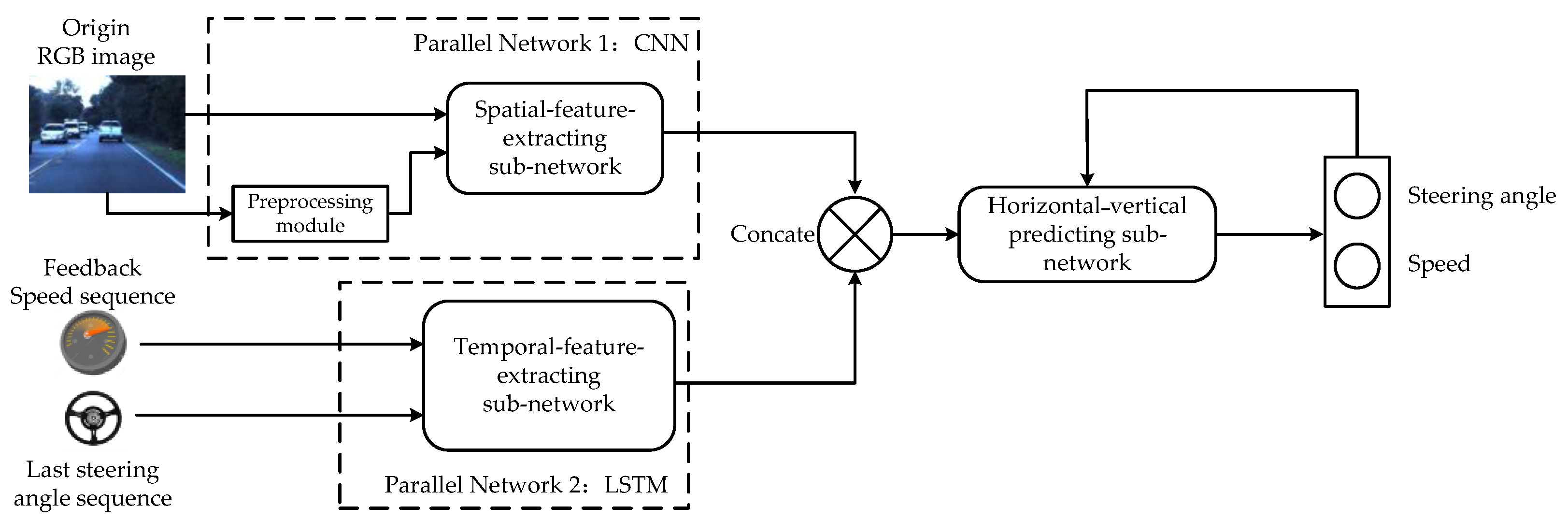
4. Proposed Method: DP-Net

For statement clarity, we conceptually segment the proposed double parallel network (DP-Net) into three sub-networks with complementary functionalities. As shown in Figure 1, the original red (R), green (G), blue (B) image and processed image are fed into the first-parallel network. Through a spatial-feature-extracting sub-network, we catch a fixed-dimension feature representation that succinctly models the complex light visual surroundings of a car. At the same time, the steering angle sequence and speed sequence are fed into the second parallel network. A temporal-feature-extracting sub-network generates the same fixed-dimension feature representation that succinctly models the continuous kinematics internal status of a car. The temporal and spatial features extracted above are all further passed to the longitudinal and lateral prediction sub-network, which contribute to the multitask prediction of steering angle and speed.

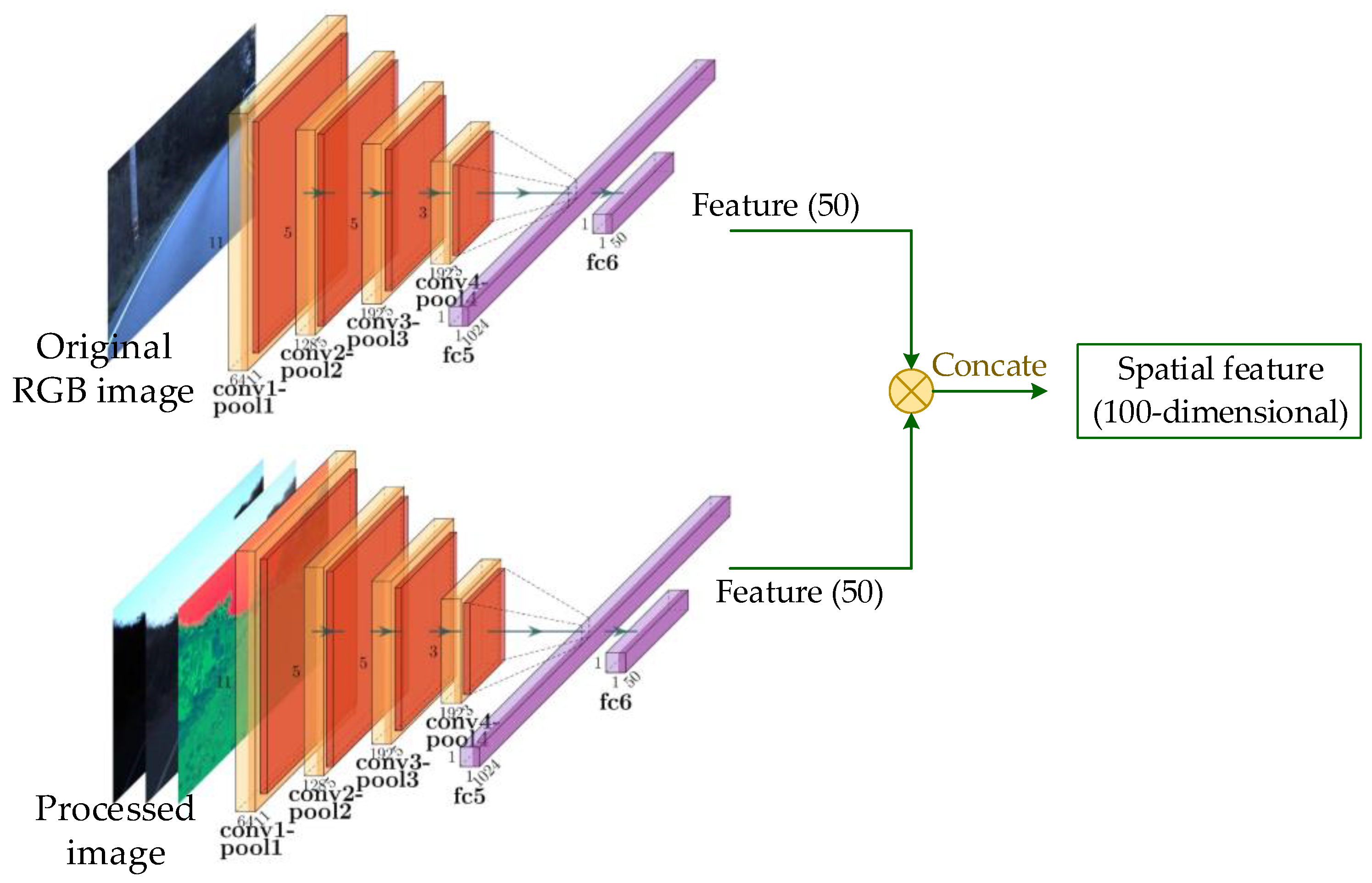
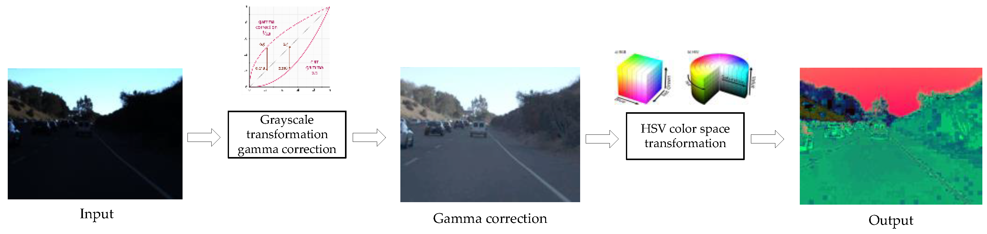
4.1. Spatial-Feature-Extracting Sub-Network

Figure 2 provides an anatomy of the spatial-feature-extracting sub-network. This sub-network is designed to handle visual perception under complex lighting conditions. To ensure that the sub-network can fully extract multiple types of spatial features, first, we create an image preprocessing module.

Preprocessing Module. The RGB images, which represent the colors of the three channels of red (R), green (G), and blue (B), show color images using different color components. However, the acquired lane images’ quality can become poor due to insufficient light at night or in low-light road environments. As a result, there is no apparent difference between the lane lines and the background in the original RGB ones, when using sub-networks to directly extract spatial features from the raw RGB lane images collected at night, which leads to insufficient capture of semantic information. Inspired by image enhancement algorithms, we use grayscale transformation [8] to increase the contrast between lane lines and the road surface, as well as HSV color space transformation [19] to improve the robustness of illumination. In fact, grayscale transformation mainly converts the input image into the output image through specific pixel operation rules. It does not change the spatial relationship of the input image. Once the grayscale transformation function T is determined, the grayscale transformation g($·$) is also defined as follows:

$$g\left(x,y\right)=T\left[f\left(x,y\right)\right]$$

(4)

Meanwhile, the HSV color space represents hue (H), saturation (S), and value (V), and, therefore, as compared with RGB images, HSV images are more consistent with human intuition in regard to color.

In summary, as shown in Figure 3, the original RGB image and the preprocessed image are used as the dual inputs of the parallel CNN described in the following subsection, which facilitates the subsequent perception of complex illumination.

Parallel CNN Design. It has been demonstrated that, based on AlexNet [20,21], the performance of a CNN designed by Yang Z et al. [11] had a good ability for extracting visual features and it was capable of directly regressing the steering angle from raw pixels. As shown in Figure 2, we propose an improved CNN structure for this task with two improvements to research complex light and structured scenes. To fully extract the multidimensional features of complex illuminated lane images, we constructed a single-input CNN into two dual-input parallel CNNs with the same structure. In this way, we can input both the original RGB image and the preprocessed image. As it is well known that the lane is the critical information for vehicle steering; therefore, a large kernel size (11*11) was kept in the first layer.

Another improvement involved changing the convolutional layers to four convolutional layers, four pooling layers, and four fully connected layers. As shown in Figure 2, there was an entire set of convolution kernels in each convolutional layer and each one can produce a separate two-dimensional activation map. These activation maps were stacked along the depth dimension and produced the output volume. We also reduced the number of cores to the combination of 64-128-192-192. The number of convolution cores determined the number of output volumes. Previous methods [20,21] have adopted five convolutional layers and four fully connected layers and the number of cores has been the combination of 96-256-384-384-256. Going deep is essential for deep learning. However, for each convolutional layer, its capacity for learning more complex patterns should be guaranteed [22]. Therefore, while reducing the number of convolution layers, we also reduce the number of convolution kernels accordingly. The spatial feature extraction subnet finally outputs 100-dimensional visual information. Then, we fused it and used it for multitask prediction in the longitudinal and lateral prediction subnets below. The experiments show that these two improvements (multidimensional inputs and new convolution parameters) do improve the accuracy of steering angle prediction in structured scenes under complex lighting.

4.2. Temporal-Feature-Extracting Sub-Network

Figure 4 shows the anatomy of the temporal-feature-extracting sub-network. This sub-network is designed to capture temporal features of continuous vehicle kinematic transitions such as steering angle sequences and speed sequences.

The steering angle prediction network in [11] only used a single frame image as input. However, in our research project, the driving strategy of the steering angle of the multi-axle self-driving transport vehicle is related to the input image and also the steering angle at the last moment. The steering angles are continuous values in the time dimension. We used recurrent neural networks to capture the temporal dependence in steering angle sequence, which can improve the accuracy of steering angle prediction in the dark and improve the stability of self-driving transport vehicles.

In fact, both the steering angle of the lateral control and the speed value of the longitudinal control [23,24] affect the driving strategy of self-driving transport vehicles. The vehicle speed in driving depends on various factors, including the driver’s habits, the surrounding traffic conditions, road conditions, etc. The above factors cannot be reflected by the front view camera alone. Therefore, in this study, the feedback speed sequences, which are set to additional auxiliary kinematic information, also input into the model. The recurrent neural networks also capture the temporal dependence in speed sequences, improving speed prediction accuracy and achieving longitudinal control of autonomous vehicles.

LSTM is a variant of recurrent neural networks, which can capture long-term time-dependent information [25]. Therefore, in this study, the single-input LSTM based on [11] is improved to two double-input parallel LSTMs with the same structure to facilitate the extraction of temporal features between steering angle sequences and speed sequences simultaneously. As seen in Figure 4, the internal structure of the LSTM unit is illustrated by the dashed rectangular box, where $x_t$ denotes the input to the LSTM cell at the moment $t$; $c_t$ denotes the cell state, which records the information passed over time; $i_t$ denotes the input gate that determines how much information $x_t$ inputs to the current cell state $c_t$; $f_t$ denotes the forgetting gate that determines how much information is retained by the cell state $c_{t-1}$ to $c_t$ at the last moment; $o_t$ denotes the output gate that controls how much information $c_t$ passes to the output $h_t$ of the current state; $h_{t-1}$ indicates the output at the moment; and $m_t$ is the state candidate value.

LSTM controls the cell state through the gating unit. First, the forgetting gate decides what information to discard from the cell state based on the previous moment output $h_{t-1}$ and the current input $x_t$ by generating the forgetting probability $f_t$ through the sigmoid layer. Secondly, new information to update the cell state is generated in the following two steps: in the first step, the input gate determines the information $i_t$ that needs to be updated by a sigmoid layer, and in the second step, a tanh layer will be used to generate the state candidates $m_t$. Multiply the cell state at the previous moment $f_t$ and add $i_t\odot m_t$ to get the new cell state $c_t$. Last but not least, the output information is decided. The output gate is passed through the sigmoid layer to obtain the initial output $o_t$, and then the new cell state $c_t$ is processed by the tanh function and multiplied with the current output $h_t$. The working principle is shown in Equations (5)–(10) as follows:

$$i_t=\sigma \left(W_{xi}{x}_t+W_{hi}{h}_{t-1}+b_i\right)$$

(5)

$$f_t=\sigma \left(W_{xf}{x}_t+W_{hf}{h}_{t-1}+b_f\right)$$

(6)

$$o_t=\sigma \left(W_{xo}{x}_t+W_{ho}{h}_{t-1}+b_o\right)$$

(7)

$$m_t=\mathit{tan}h\left(W_{xm}{x}_t+W_{hm}{h}_{t-1}+b_m\right)$$

(8)

$$c_t=f_t\odot c_{t-1}+i_t\odot m_t$$

(9)

$$h_t=o_t\odot \mathit{tan}h\left(c_t\right)$$

(10)

where w and b denote the weight vector and offset of the corresponding gating unit, respectively; $\sigma (•)$ denotes the sigmoid activation function; $\mathit{tan}h(•)$ denotes the hyperbolic tangent activation function; and $\odot$ denotes the Hadamard product.

As shown in Figure 4, the input $x_t$ to the LSTM unit represents the steering angle sequence or speed sequence. At moment $t$, the previous LSTM cell output $h_{t-1}$, the cell state $c_{t-1}$, as well as $x_t$, are input to the LSTM cell to obtain the temporal feature output $h_t$ of the current moment. Finally, the temporal feature extraction sub-network outputs two 100-dimensional vehicle dynamics information. Next, we will merge them in the longitudinal and lateral prediction sub-networks, described below, and use them for multitask prediction.

4.3. Longitudinal and Lateral Prediction Sub-Network

Figure 5 depicts our proposed longitudinal and lateral prediction sub-network. It fuses several kinds of temporal information and space information at multiple network layers.

As shown in Figure 5a, the longitudinal and lateral control networks predict the driving strategy based on the new fusion features. We propose a longitudinal and lateral prediction sub-network which consists of feature fusion (merge) layers and fully connected layers. Unlike Yang Z [11] who fused only speed sequence features, in this study, we separately fuse visual features and vehicle kinematic features (steering angle and speed) in the feature merge layer. In fact, the excellent results achieved by ResNet [26] in image classification areas also demonstrate that feature fusion can enhance network learning, improve the expressiveness of the network, and help the model converge more accurately and faster. In the merged layer, the method is feature cascading (concatenate), as Figure 5b shows. Feature cascade is the stitching of the feature vectors output from two branch networks, and the newly generated features are the result of concatenating the two feature vectors. Different from feature summation, a simple superposition, the dimensions of the new feature vector generated by feature cascading can be significantly increased.

Two 100-dimensional feature vectors, separately output from the spatial feature extraction network and the temporal feature extraction network, are stitched together to generate 200 high-dimensional features. The new feature vectors are passed to the fully connected layers, where the numbers of neurons in the four fully connected layers of the lateral prediction network are 200, 100, 50, and 1. Additionally, the longitudinal prediction network parameters are the same as above. Finally, the steering angle and speed are simultaneously output to achieve the self-driving transport vehicle’s lateral and longitudinal decision making.

5. Experiments Evaluation

5.1. Experiments Setup

Dataset Description. We perform evaluations on the standard benchmarks that are widely used in the community; namely, Udacity Challenge II [27]. The Udacity dataset is mainly composed of video frames taken from structured urban roads and it contains multiple frames of severe lighting changes. As shown in Figure 6, it fits our model research scenario. Specifically, data-collecting cars have three cameras mounted at the left/middle/right around the rear mirror. Videos are captured at a rate of 20 FPS. For each video frame, the data provider managed to record corresponding geo-location (latitude and longitude), timestamp (in millisecond), and vehicle states (wheel angle, torque, and driving speed). Recalling the previously designed double parallel network DP-Net, the video frame input of the spatial feature extraction subnet and vehicle state input (steering angle, speed) of the temporal feature extraction subnet, are precisely provided by the Udacity Challenge II dataset.

Network Optimization. The experiments are conducted on the Intel(R) Core(TM) i7-8700CPU and NVIDIA GeForce GTX1660 GPU. All code is written in Google’s TensorFlow framework. The following are some crucial parameters for reimplementing our method: dropout with a ratio of 0.5 is used in fully connected layers; the learning rate is initialized to 1 × 10⁻⁴ and halved when the objective is stuck in some plateau. We randomly draw 5% of the data set for validating models and always retain the best model on the whole validation process. We adopt ADAM [28] for the stochastic gradient solver, which is an algorithm for first-order gradient-based optimization of stochastic objective functions. Model training requires about 20 h over the GPU. Inspired by AlexNet’s LRN [21], and in order to improve the generalization ability of the network, we introduce Batch normalization after the convolutional layer [29].

In neural networks, the loss function is used to measure the difference between the predicted value and the ground truth value. We define two types of loss items in the preliminary prediction task; namely, $L_{steer}$ and $L_{speed}$. The steering angle prediction loss $L_{steer}$ is described in Equation (2) and the speed prediction loss $L_{speed}$ is defined in Equation (3).

In addition, we add the mean absolute error (MAE) as metrics to monitor the model performance, which can better reflect the actual prediction value error. Therefore, the final objective function is described as:

$$L=\underset{\mathrm{steering}\mathrm{loss}}{\underbrace{L_{steer}\left(p_1,{\widehat{p}}_1\right)}}+\underset{\mathrm{speeding}\mathrm{loss}}{\underbrace{L_{speed}\left(p_2,{\widehat{p}}_2\right)}}$$

(11)

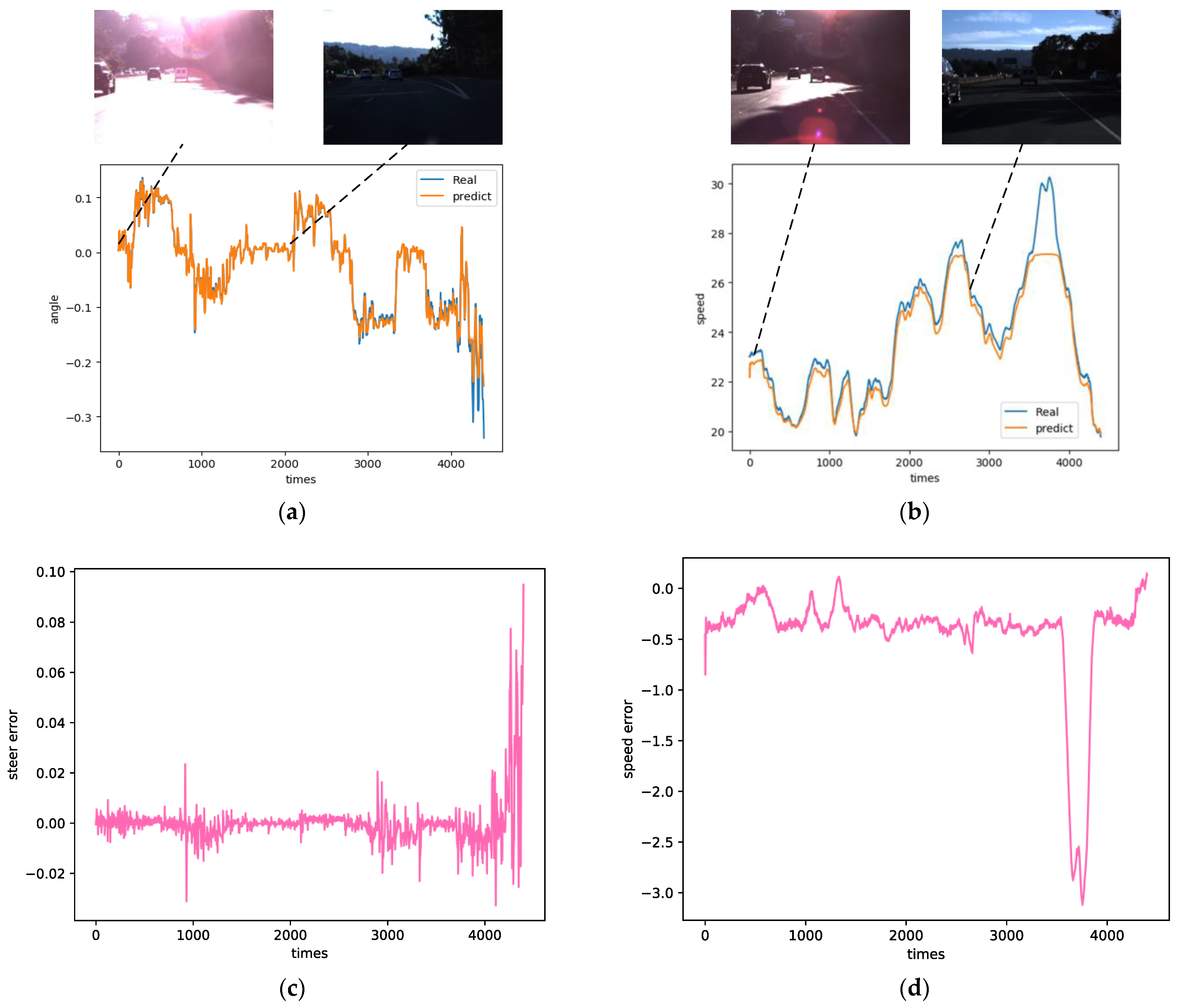
5.2. Performance Analysis

5.2.1. Comparison with Competing Algorithms

First, we evaluate the performance of the end-to-end steering angle prediction. We compare the proposed DP-Net with several competing algorithms. Brief descriptions of these competitors are given below:

• PilotNet is the network proposed by NVIDIA. It consists of five convolutional layers and five fully connected layers, which use small kernel sizes (3 × 3, 5 × 5). We re-implemented this according to NVIDIA’s original technical report. All input video frames are resized to 200 × 66 before feeding PilotNet.
• CgNet is an open-source model with an excellent ranking in the Udacity Challenge II. Compared with PilotNet, it adjusts the kernel parameters to use only three convolutional layers and two fully connected layers, and it only uses a small kernel size (3 × 3). Note that the input of both PilotNet and CgNet is only the original single frame image, which ignores the visual features in dark light.
• The E2E multimodal multitask network is a five-layer convolution and four-layer fully connected multimodal multitask network, based on the AlexNet architecture proposed by Yang Z et al. We re-implemented it on Udacity Challenge II, according to the authors’ paper. Note that, although the authors extracted the temporal features by the LSTM network, it was not passed and applied to predict the steering angle. Therefore, the internal continuous kinematic state of the vehicle is ignored.

In this section, we evaluate the performance of the proposed DP-Net, which merges the visual and kinematic features extracted by the double parallel network, sequentially, to predict lateral steering angle. First, we focus on predicting the steering angle. The RMSE (root mean squared error) and the MAE of steering angles are shown in

Table 1. Experimental results of steering angle prediction on Udacity Challenge II.

Method	RMSE	MAE	Max Prediction Error
Nvidia’s PilotNet	0.3063	0.2213	0.4973
Cg Net	0.3096	0.2219	0.4958
E2E multimodal multitask network	0.0584	0.0163	0.2732
Proposed DP-Net (ours)	0.0107	0.0054	0.0948

, from which we have several immediate observations.

First, image preprocessing and the input of multidimensional image features heavily correlate to the final performance. In particular, image enhancement and HSV color space conversion exhibit advantages for representing complex lighting conditions. It is well known that lane lines are an essential feature of structured roads. We increase the contrast between the lane lines and the road surface in the image through our image preprocessing module. Then, we merge the original RGB image features and HSV spatial color features for the lateral prediction sub-network. Compared to competing algorithms with single raw image feature inputs, our network has significantly better accuracy and robustness. To further investigate the experimental results, Figure 7a plots the steering angles in a testing video sequence. We also take two sub-nodes (t = 3 and t = 1840), which correspond to the intense light and dark light road scenes on the road, as shown in the scenes plotted in Figure 7a. Clearly, our model (the orange curve) predicts very accurately. As shown in Figure 7c, the basic steer angle errors between the predicted and the Udacity dataset values are limited to ±0.02. Additionally, we will try to use transfer learning to deal with individual errors during subsequences (t = 4000~4300) in future research.

Secondly, besides the input of multidimensional visual features, our model also clearly differs from others by fusing vehicle kinematic features. Inspired by the kinematic modeling of traditional decision algorithms, we conjecture that it is inherently difficult to predict the steering angle with visual input alone. Therefore, we add the steering angle sequence of the previous ten frames as the model’s physical constraints. As shown in Table 1, it is apparent that the RMSE and MAE of proposed DP-Net are reduced from 0.3063 and 0.2213 to 0.0107 and 0.0054 as compared with NVIDIA PilotNet. Noticeably, compared with E2E multimodal multitask network, we reduce the RMSE by 81.7% (from 0.0584 to 0.0107), the MAE by 66.9% (from 0.0163 to 0.0054), and the maximum prediction error by 65.3% (from 0.2732 to 0.0948). This shows that the additional vehicle kinematic information, from the steering angle sequence, provides richer and more comprehensive inputs. It improves the continuity of steering angle prediction and reduces the jerking of the vehicle’s steering wheel. As can be seen from Table 1, it is clear that our experimental results verify the directional effects of the conjecture. Additionally, our results provide some ideas for more vehicle dynamic information such as position and attitude of multi-axle transport vehicles in subsequent fusion projects, which we further described through an ablation analysis.

Lastly, different from PilotNet, CgNet with small convolutional kernels, and E2E multimodal multitask network with AlexNet structure, we have designed a new combination of convolutional kernel size and number, which we further consider in a subsequent ablation analysis.

The proposed DP network once again merges the continuous extracted visual and kinematic features, subsequently to predict the longitudinal speed through the double parallel network. Similar to the regression task for the steering angle, we also analyzed the performance of the model in terms of root mean square error (RMSE) and mean absolute error (MAE) of the speed. For the CNN model, the predicted speed bias is larger when only a single image frame is input. Therefore, we did not do a comparative analysis of PilotNet and CgNet in

Table 2. Experimental results of speed prediction on Udacity Challenge II.

Method	RMSE	MAE	Max Prediction Errors
E2E multimodal multitask network	1.7112	0.13	−3.0250
Proposed DP-Net (ours)	1.4211	0.8802	−3.1101

. We only choose the E2E multimodal multitask network results as a baseline for comparison.

As can be seen from Table 2, the RMSE is reduced from 1.7112 to 1.4211, a relative improvement of 17%. To further evaluate the overall effectiveness of the proposed DP-Net experimental results, Figure 7b plots the speed in 4400 frames from the test set. The orange curve in the graph indicates the ground truth curve and the blue curve indicates the prediction curve. It can be observed that the speed prediction results and the predicted values match well with the ground truth. The basic speed errors between the predicted and the Udacity dataset values fluctuate around 0.5, as shown in Figure 7d. This indicates that the improved parallel CNN network can extract richer visual features and can merge them with the temporal contextual features of the speed sequence by the LSTM network to generate new high-level semantic features. Therefore, our network can better facilitate the learning of the longitudinal decision network, narrowing the gap between the prediction and ground truth values of speed.

However, as shown in

Table 3. Experimental results of steering angle and speed with different convolution kernels numbers.

Number of Convolution Kernels	RMSE		MAE
	Steering Angle	Speed	Steering Angle	Speed
48-64-128-128	0.0251	1.8057	0.0202	1.3895
64-128-128-128	0.0235	2.0441	0.019	1.6535
64-128-128-192	0.0242	2.0208	0.0191	1.489
64-128-192-192	0.0107	1.4211	0.0054	0.8802
128-128-192-192	0.0301	2.7121	0.027	2.2623
128-128-192-256	0.0021	2.3474	0.0404	2.0307

, the proposed DP-Net’s MAE and maximum prediction errors are not satisfactory. We conjecture that because MAE gives each error value the same weight, some abnormal speed points in the test set cannot be well predicted. The subsequent t = 3500 to approximately t = 4000, in Figure 7b, also confirm our conjecture. Therefore, attention should be focused on the handling and prediction of speed outliers when our model is subsequently deployed to actual multi-axle transport vehicles.

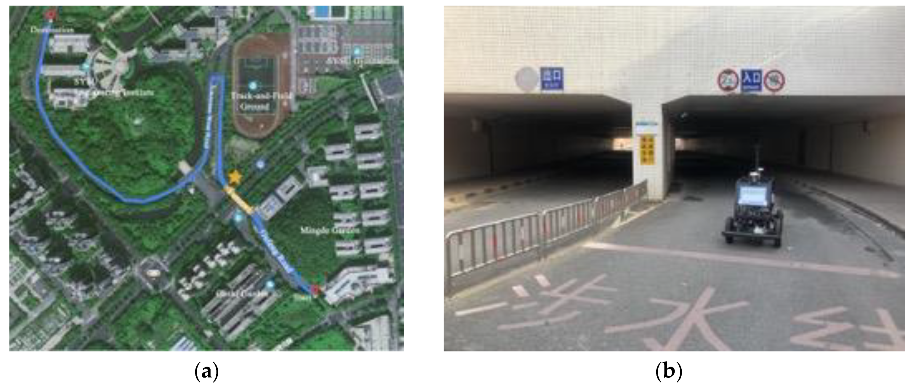
5.2.2. Validation on SYSU Campus

Safety is always regarded as a top priority in autonomous driving. Therefore, to ensure that the proposed DP-Net can subsequently be safely and accurately deployed to our multi-axle transport vehicle project, it is necessary to test it on a real-world dataset. Ideally, the training model has an accurate predictive effect on the steering angle and speed of the test set.

We recorded and constructed the SYSU Campus dataset collected by Baidu’s Apollo D-KIT Lite [30]. The dataset includes two hours of driving data from the Gufeng Road and Xiaoyuan West Road on campus, with clear road edges. The routing and some frame images of the dataset are shown in Figure 8. The dataset contains the driving data in both normal daylight and dark tunnel night. Similar to the structure of the Udacity Challenge II dataset, speed values and steering angles are recorded. The video streams contain videos from one center and two side front view cameras with a frame rate of 20 frames per second.

In order to visualize the longitudinal and lateral test results of the proposed DP-Net (choosing a combination of 64-128-192-192), we prepared six representative key test video frames before, during, and after entering and exiting the tunnel, shown in Figure 9. It is observed that the predictions of steering angle and speed are very close to the ground truth values, which indicates that the learned model indeed captures the critical factor in complex lighting such as tunnels. To further evaluate the overall effectiveness of the longitudinal and lateral prediction results, Figure 10 plots the curves in 8000 frames from the SYSU Campus dataset. The orange curve in the graph indicates the ground truth and the blue curve shows the prediction value. For the steering angle, our model (orange curve) predicts it very accurately; for the speed values, as conjectured above, the predicted values are limited. Therefore, transfer learning on the actual dataset could be a good optimization idea to deploy the model on the multi-axle real vehicle in our subsequent project.

5.3. Ablation Analysis

Our proposed model includes two novel designs, i.e., large convolutional kernels and small convolutional kernel numbers. First, based on the original dataset of 640 × 480 pixels, in order to better extract the underlying features in the image, we design a large convolution kernel size (11 × 11) to obtain a larger perceptual field [31]. Secondly, the higher the number of convolutional kernels, the more feature information can be extracted for learning. However, this also causes the network parameters to increase abruptly, slowing down the computation and overfitting during the training process [23]. This section presents an ablative experiment to quantitatively evaluate the effect of different combinations of convolution kernel numbers. Specifically, we tested six combinations of the number of convolutional kernels from small to large. The goal was to verify the effect of the factor on the final accuracy.

The results of these evaluations are shown in Table 3. The table shows that a moderate number of convolutional kernels provides us with optimal accuracy. Inspired by the idea in [23,32], the task of designing deeper networks and a more significant number of convolutional kernels is essentially a constrained optimization problem. In the lane perception task of this study, for each convolutional layer, its capacity of learning more complex patterns should be guaranteed. Therefore, at this point, it is not suitable and unreasonable to use too many convolution kernels and too deep networks.

According to the above 64-128-192-192 convolution kernel parameters, we further designed controlled experiments to compare the network’s performance, considering different information. The results are shown in

Table 4. Controlled experimental results of steering angle and speed considering only image data (convolutional neural network, CNN) and considering both image data (CNN) and kinematics data (LSTM).

Method	RMSE		MAE
	Steering Angle	Speed	Steering Angle	Speed
CNN	0.0301	3.3778	0.0243	2.7171
CNN-LSTM (DP-Net)	0.0107	1.4211	0.0054	0.8802

. It shows that the visual information (such as the edge of roads and lane lines) and previous vehicle kinematics state (steering angle and speed) provide crucial information for the task that we are considering. In terms of steering angle, the RMSE and MAE of CNN-LSTM (DP-Net) are reduced from 0.0301 and 0.0243 to 0.0107 and 0.0054 as compared with CNN. This shows that the additional vehicle kinematic information improves the continuity of steering angle prediction and it also reduces the jerking of the vehicle’s steering wheel. In terms of speed, it is apparent that the RMSE and MAE of CNN-LSTM (DP-Net) are reduced from 3.3778 and 2.7171 to 1.4211 and 0.8802, as compared with CNN. It shows that the LSTM networks capture the temporal dependence in speed sequences, improving speed prediction accuracy and achieving the longitudinal control of autonomous vehicles. Therefore, it is possible to enhance the network to multi-parallel to fuse more vehicle kinematics information, such as position and attitude of multi-axle transport vehicles in our subsequent project.

6. Conclusions

In this study, we have solved the task of end-to-end vehicle lateral and longitudinal driving strategy in terms of the speed and steering angle. Aiming at the complex illumination (tunnel) of structured scenarios in autonomous driving, a double parallel network is proposed. In feature extraction and perception, a preprocessing module is presented to ensure adequate visual information extraction under complex illumination. Then, a parallel CNN sub-network and a parallel LSTM sub-network are designed. The parallel LSTM sub-network uses vehicle kinematic features as physical constraints to help predict acceleration more accurately.

The experimental results show that our proposed DP-Net can accurately predict steering angle and speed, and further improve the robustness of complex illumination and the accuracy of lateral and longitudinal prediction. In addition, a new SYSU Campus dataset is collected for evaluation and testing. However, the more complex kinematic characteristics (multi-axle steering angles, position, and pose) of the multi-axle transport vehicle are not considered in our approach. Moreover, due to the different distributions between the training datasets and test datasets, the prediction of speed by the DP-Net, in this study, is not sufficiently accurate. Subsequent proposed research work should include the following: (1) incorporating more kinematic features of multi-axle vehicles in feature extraction and perception and (2) using transfer learning to further improve the accuracy of longitudinal speed prediction values.

References

1. Park, B.; Lee, Y.-C.; Han, W.Y. Trajectory generation method using Bezier spiral curves for high-speed on-road autonomous vehicles. In Proceedings of the 2014 IEEE International Conference on Automation Science and Engineering (CASE), Taipei, Taiwan, 18–22 August 2014; pp. 927–932. [Google Scholar]
2. Ziegler, J.; Bender, P.; Dang, T.; Stiller, C. Trajectory planning for Bertha A local, continuous method. In Proceedings of the 2014 IEEE Intelligent Vehicles Symposium Proceedings, Dearborn, MI, USA, 8–11 June 2014; pp. 450–457. [Google Scholar]
3. Simonyan, K.; Zisserman, A. Very deep convolutional networks for large-scale image recognition. arXiv 2014, arXiv:1409.1556. [Google Scholar]
4. Cun, Y.L.; Boser, B.; Denker, J.S.; Henderson, D.; Jackel, L.D. Handwritten digit recognition with a back-propagation network. Adv. Neural Inf. Process. Syst. 1990, 2, 396–404. [Google Scholar]
5. Bojarski, M.; Del Testa, D.; Dworakowski, D. End to end learning for self-driving cars. arXiv 2016, arXiv:1604.07316. [Google Scholar]
6. Xu, H.; Gao, Y.; Yu, F.; Darrell, T. End-to-End Learning of Driving Models from Large-scale Video Datasets. In Proceedings of the 30th IEEE/CVF Conference on Computer Vision and Pattern Recognition (CVPR), Honolulu, HI, USA, 21–26 July 2017; pp. 3530–3538. [Google Scholar]
7. Pomerleau, D.A. Alvinn: An Autonomous Land Vehicle in a Neural Network. In Proceedings of the 1st Neural Information Processing Systems (NIPS Conference), Denver, CO, USA, 27–30 November 1988; pp. 305–313. [Google Scholar]
8. Luo, Q.; Wang, G.Y.; Chu, W.D. Lane detection in micro-traffic under complex illumination. Comput. Sci. 2014, 41, 46–49. (In Chinese) [Google Scholar]
9. Chi, L.; Mu, Y. Deep steering: Learning end-to-end driving model from spatial and temporal visual cues. arXiv 2017, arXiv:1708.03798. [Google Scholar]
10. Codevilla, F.; Miiller, M.; Lopez, A.; Koltun, V.; Dosovitskiy, A. End-to-End Driving Via Conditional Imitation Learning. In Proceedings of the 2018 IEEE International Conference on Robotics and Automation (ICRA), Brisbane, Australia, 21–25 May 2018; pp. 1–9. [Google Scholar]
11. Yang, Z.; Zhang, Y.; Yu, J. End-to-end Multi-Modal Multi-Task Vehicle Control for Self-Driving Cars with Visual Perceptions. In Proceedings of the 24th International Conference on Pattern Recognition (ICPR), Beijing, China, 20–24 August 2018; pp. 2289–2294. [Google Scholar]
12. Hou, Y.; Ma, Z.; Liu, C.; Loy, C.C. Learning to Steer by Mimicking Features from Heterogeneous Auxiliary Networks. In Proceedings of the 33rd AAAI Conference on Artificial Intelligence/31st Innovative Applications of Artificial Intelligence Conference/9th AAAI Symposium on Educational Advances in Artificial Intelligence, Honolulu, HI, USA, 27 January–1 February 2019; pp. 8433–8440. [Google Scholar]
13. Eraqi, H.M.; Moustafa, M.N.; Honer, J. End-to-End Deep Learning for Steering Autonomous Vehicles Considering Temporal Dependencies. In Proceedings of the 31st Conference on Neural Information Processing Systems (NIPS), Long Beach, CA, USA, 4–9 December 2017. [Google Scholar]
14. Hecker, S.; Dai, D.; Van Gool, L. End-to-End Learning of Driving Models with Surround-view Cameras and Route Planners. In Proceedings of the 15th European Conference on Computer Vision (ECCV), Munich, Germany, 8–14 September 2018; pp. 449–468. [Google Scholar]
15. Roh, C.G.; Im, I.J. A review on handicap sections and situations to improve driving safety of automated vehicles. Sustainability 2020, 12, 5509. [Google Scholar] [CrossRef]
16. Nalic, D.; Pandurevic, A.; Eichberger, A.; Rogic, B. Design and Implementation of a Co-Simulation Framework for Testing of Automated Driving Systems. Sustainability 2020, 12, 10476. [Google Scholar] [CrossRef]
17. Chen, C.; Seff, A.; Kornhauser, A.; Xiao, J. Deep Driving: Learning affordance for direct perception in autonomous driving. In Proceedings of the IEEE International Conference on Computer Vision (ICCV), Santiago, Chile, 11–18 December 2015; pp. 2722–2730. [Google Scholar]
18. Paliwal, S. Identity verification using speech and face information. Digit. Signal Process. 2004, 14, 449–480. [Google Scholar]
19. Krizhevsky, A.; Sutskever, I.; Hinton, G.E. Imagenet classification with deep convolutional neural networks. Adv. Neural Inf. Process. Syst. 2012, 25, 1097–1105. [Google Scholar] [CrossRef]
20. Jia, Y.; Shelhamer, E.; Donahue, J.; Karayev, S.; Long, L.R.; Girshick, S.; Guadarrama, T.D. Caffe: Convolutional architecture for fast feature embedding. In Proceedings of the ACM Conference on Multimedia (MM), Orlando, FL, USA, 3–7 November 2014; pp. 675–678. [Google Scholar]
21. Cao, X. A Practical Theory for Designing Very Deep Convolutional Neural Networks. Unpublished Technical Report. 2015. Available online: https://www.kaggle.com/blobs/download/forum-message-attachment-files/2287/A%20practical%20theory%20for%20designing%20very%20deep%20convolutional%20neural%20networks.pdf (accessed on 24 November 2020).
22. Xiong, H.; Zhu, X.; Zhang, R. Energy Recovery Strategy Numerical Simulation for Dual Axle Drive Pure Electric Vehicle Based on Motor Loss Model and Big Data Calculation. Complexity 2018, 2018, 1–14. [Google Scholar] [CrossRef] [Green Version]
23. Zhang, R.-H.; He, Z.-C.; Wang, H.-W.; You, F.; Li, K.-N. Study on Self-Tuning Tyre Friction Control for Developing Main-Servo Loop Integrated Chassis Control System. IEEE Access 2017, 5, 6649–6660. [Google Scholar] [CrossRef]
24. Wojna, Z.; Gorban, A.N.; Lee, D.-S.; Murphy, K.; Yu, Q.; Li, Y.; Ibarz, J. Attention-Based Extraction of Structured Information from Street View Imagery. In Proceedings of the 2017 14th IAPR International Conference on Document Analysis and Recognition (ICDAR), Kyoto, Japan, 9–15 November 2017; Volume 1, pp. 844–850. [Google Scholar]
25. Hochreiter, S.; Schmidhuber, J. Long Short-Term Memory. Neural Comput. 1997, 9, 1735–1780. [Google Scholar] [CrossRef] [PubMed]
26. He, K.; Zhang, X.; Ren, S.; Sun, J. Deep residual learning for image recognition. arXiv 2015, arXiv:1512.03385. [Google Scholar]
27. UDACITY. Available online: https://www.udacity.com/self-driving-car (accessed on 28 October 2020).
28. Kingma, D.P.; Ba, J. Adam: A method for stochastic optimization. arXiv 2014, arXiv:1412.6980. [Google Scholar]
29. Ioffe, S.; Szegedy, C. Batch normalization: Accelerating deep network training by reducing internal covariate shift. arXiv 2015, arXiv:1502.03167. [Google Scholar]
30. Baidu Autonomous Driving Development Kit (Apollo D-KIT). Available online: https://apollo.auto/apollo_d_kit.html (accessed on 24 November 2020).
31. Peng, C.; Zhang, X.; Yu, G.; Luo, G.; Sun, J. Large Kernel Matters—Improve Semantic Segmentation by Global Convolutional Network. In Proceedings of the 2017 IEEE Conference on Computer Vision and Pattern Recognition (CVPR), Honolulu, HI, USA, 21–26 July 2017; pp. 1743–1751. [Google Scholar]
32. Sun, X.; Hong, Z.; Meng, W.; Zhang, R.; Li, K.; Tao, P. Primary resonance analysis and vibration suppression for the harmonically excited non-linear suspension system using a pair of symmetric viscoelastic buffers. Nonlinear Dyn. 2018, 94, 1243–1265. [Google Scholar] [CrossRef]
Figure 1. The architecture of our proposed double parallel networks for the predicting task of steering angle and speed. The arrows in the network denote the direction of data forwarding.
Sustainability 13 04531 g001
Figure 2. The design of spatial-feature-extracting sub-network. The proposed sub-network enjoys several unique traits, including parallel structure, larger convolution kernel, and a smaller number of convolution kernels.
Sustainability 13 04531 g002
Figure 3. The design of the preprocessing module. The original RGB dark load is converted by the nonlinear grayscale transformation function (gamma correction = 0.35) and color space transformation to output a hue saturation value (HSV) image.
Sustainability 13 04531 g003
Figure 4. Data flow in the long short-term memory network (LSTM) network. The network reads output in the previous step, including speed and steering angle, as described before. We set T (the length of historical data) as 10.
Sustainability 13 04531 g004
Figure 5. Longitudinal and lateral predicting sub-network. (a) Separately fuse the speed temporal feature (upper) and the steer temporal feature (under) with the spatial feature; (b) feature vectors concatenate.
Sustainability 13 04531 g005
Figure 6. Example video frames in the Udacity Challenge II dataset.
Sustainability 13 04531 g006
Figure 7. The proposed DP-Net performance on the Udacity Challenge II dataset. (a) Steering angle prediction results. The selected sub-nodes are highlighted such that more detailed differences can be observed; (b) speed value prediction results; (c) the steer angle errors between the predicted and the dataset values; (d) the speed errors between the predicted and the dataset values.
Sustainability 13 04531 g007
Figure 8. We collect the test dataset in SYSU Campus. (a) The start and endpoints are marked with red dots, and the location of the tunnel is marked with yellow lines; (b) the collected details.
Sustainability 13 04531 g008
Figure 9. We select representative scenarios from the testing video sequence. Ground truth (displayed in green) and our predictions (in yellow) are both imposed on the video frames. Note that our predictions are nearly identical to the ground truth in these challenging inputs. (a) before entering the tunnel; (b) About to enter the tunnel; (c) In the tunnel; (d) continuous driving in the tunnel; (e) coming out of the tunnel; (f) driving out of the tunnel.
Sustainability 13 04531 g009aSustainability 13 04531 g009b
Figure 10. The proposed DP-Net performance on the SYSU campus dataset. (a) Steering angle prediction results; (b) speed value prediction results; (c) the steer angle error between the predicted and the dataset values; (d) the speed error between the predicted and the dataset values.
Sustainability 13 04531 g010