
Multimetric Index to Evaluate Water Quality in Lagoons: A Biological and Geomorphological Approach

 , ,
, ,
Abstract
:1. Introduction
2. Multimetric Index Conceptualization
2.1. Preliminaries
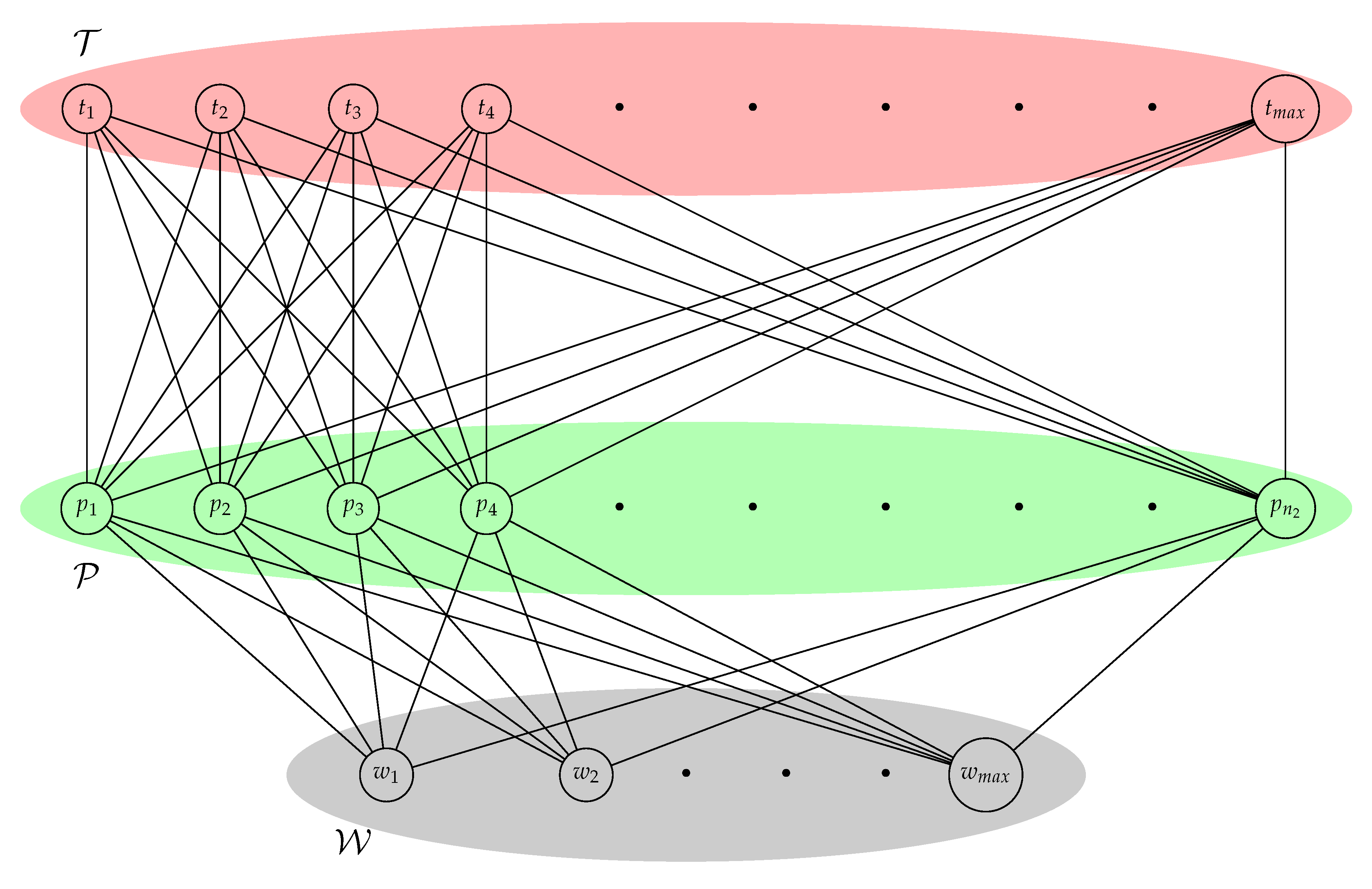
2.2. JP(G) Index
2.3. Macrophytes Quality Index MQI
2.4. Morphological Quality Index MoQI
3. Analyzing the MMI
4. Comparison between Indices to Study Water Quality
5. Structural Analysis of the Geometric Model
6. Conclusions
Author Contributions
Funding
Institutional Review Board Statement
Informed Consent Statement
Data Availability Statement
Acknowledgments
Conflicts of Interest
References
- Muñoz-Piña, C.; Guevara, A.; Torres, J.M.; Braña, J. Paying for the Hydrological Services of Mexico’s Forests: Analysis, Negotiations and Results. Ecol. Econ. 2008, 65, 725–736. [Google Scholar] [CrossRef]
- Karr, J.R. Assessment of Biotic Integrity Using Fish Communities. Fisheries 1981, 6, 21–27. [Google Scholar] [CrossRef]
- Karr, J.R. Defining and measuring river health. Freshw. Biol. 1999, 41, 221–234. [Google Scholar] [CrossRef] [Green Version]
- Furse, M.T.; Hering, D.; Brabec, K.; Buffagni, A.; Sandin, L.; Verdonschot, P.F. The ecological status of European rivers: Evaluation and intercalibration of assessment methods. Hydrobiologia 2006, 566, 1–2. [Google Scholar] [CrossRef] [Green Version]
- Resh, V.H.; Norris, R.H.; Barbour, M.T. Design and implementation of rapid assessment approaches for wáter resource monitoring using benthic macroinvertebrates. Austral Ecol. 1995, 20, 108–121. [Google Scholar] [CrossRef]
- Bonada, N.; Prat, N.; Resh, V.H.; Statzner, B. Developments in aquatic insect biomonitoring: A comparativeanalysis of approaches. Annu. Rev. Entomol. 2006, 51, 495–523. [Google Scholar] [CrossRef] [Green Version]
- Aazami, J.; Moradpour, H.; Zamani, A.; Kianimehr, N. Ecological quality assessment of Kor River in Fars Province using macroinvertebrates indices. Int. J. Environ. Sci. Technol. 2019, 16, 6935–6944. [Google Scholar] [CrossRef]
- Lücke, J.D.; Johnson, R.K. Detection of ecological change in stream macroinvertebrate assemblages using single metric, multimetric or multivariate approaches. Ecol. Indic. 2019, 9, 659–669. [Google Scholar] [CrossRef]
- Saloom, M.E.; Scot Duncan, R. Low dissolved oxygen levels reduce anti-predation behaviours of the freshwater clam Corbicula fluminea. Freshw. Biol. 2005, 50, 1233–1238. [Google Scholar] [CrossRef]
- Cross, W.F.; Wallace, J.B.; Rosemond, A.D.; Eggert, S.L. Whole-system nutrient enrichment increases secondary production in a detritus-based ecosystem. Ecology 2006, 87, 1556–1565. [Google Scholar] [CrossRef]
- Steinman, A.D.; Rosen, B.H. Lotic–lentic linkages associated with Lake Okeechobee, Florida. J. N. Am. Benthol. Soc. 2000, 19, 733–741. [Google Scholar] [CrossRef]
- Haury, J.; Peltre, M.C.; Trémolières, M.; Barbe, J.; Thiebaut, G.; Bernez, I.; Daniel, H.; Chatenet, P.; Haan-Archipof, G.; Muller, S.; et al. A new method to assess water trophy and organic pollution—the Macrophytes Biological Index for Rivers (IBMR): Its application to different types of river and pollution. Hydrobiologia 2006, 570, 153–158. [Google Scholar] [CrossRef]
- O’Hare, M.; Baattrup-Pedersen, A.; Nijboer, R.C.; Szoszkiewicz, K.; Ferreira, T. Macrophyte communities of European streams with altered physical habitat. Hydrobiologia 2006, 566, 197–210. [Google Scholar] [CrossRef] [Green Version]
- Demars, B.O.L.; Potts, J.M.; Tremolieres, M.; Thiebaut, G.; Gougelin, N.; Nordmann, V. River macrophyte indices: Not the Holy Grail! Freshw. Biol. 2012, 57, 1745–1759. [Google Scholar] [CrossRef]
- Muratov, R.; Zhamangara, A.; Beisenova, R.; Akbayeva, L.; Szoszkiewicz, K.; Jusik, S.; Gebler, D. An attempt to prepare Macrophyte Index for Rivers for assessment watercourses in Kazakhstan. Meteorol. Hydrol. Water Manag. Res. Oper. Appl. 2015, 3, 27–32. [Google Scholar] [CrossRef]
- Rinaldi, M.; Surian, N.; Comiti, F.; Bussettini, M.; Belletti, B.; Nardi, L.; Golfieri, B. Guidebook for the evaluation of stream morphological conditions by the Morphological Quality Index (MQI). Version 2012, 1, 85. [Google Scholar]
- Wyżga, B.; Zawiejska, J.; Radecki-Pawlik, A.; Amirowicx, A. A method for the assessment of hydromorphological river quality and its application to the Czarny Page 49 of 177 Dunajec, Polish Carpathians. In Cultural Landscapes of River Valleys; Radecki-Pawlik, A., Hernik, J., Eds.; Agricultural University in Kraków: Kraków, Poland, 2010; pp. 145–164. [Google Scholar]
- Wyżga, B.; Zawiejska, J.; Radecki-Pawlik, A.; Hajdukiewicz, H. Environmental change, hydromorphological reference conditions and the restoration of Polish Carpathian rivers. Earth Surf. Process. 2012. [Google Scholar] [CrossRef]
- Rinaldi, M.; Surian, N.; Comiti, F.; Bussettini, M. A method for the assessment and analysis of the hydromorphological condition of Italian streams: The Morphological Quality Index (MQI). Geomorphology 2013, 180–181, 96–108. [Google Scholar] [CrossRef]
- Pérez-Domínguez, R.; Maci, S.; Courrat, A.; Lepage, M.; Borja, A.; Uriarte, A.; Netoe, J.M.; Cabral, H.; Raykov, V.S.; Franco, A.; et al. Current developments on fish-based indices to assess ecological-quality status of estuaries and lagoons. Ecol. Indic. 2012, 23, 34–45. [Google Scholar] [CrossRef]
- Hawkes, H.A. Origin and development of the biological monitoring working party score system. Water Res. 1998, 32, 964–968. [Google Scholar] [CrossRef]
- Jun, Y.C.; Won, D.H.; Lee, S.H.; Kong, D.S.; Hwang, S.J. A multimetric benthic macroinvertebrate index for the assessment of stream biotic integrity in Korea. Int. J. Environ. Res. Public Health 2012, 9, 3599–3628. [Google Scholar] [CrossRef] [PubMed]
- Bazzoni, A.M.; Pulina, S.I.L.V.I.A.; Padedda, B.M.; Satta, C.T.; Lugliè, A.; Sechi, N.; Facca, C. Water quality evaluation in Mediterranean lagoons using the Multimetric Phytoplankton Index (MPI): Study cases from Sardinia. Transitional Waters Bull. 2013, 7, 64–76. [Google Scholar]
- Lucena-Moya, P.; Pardo, I. An invertebrate multimetric index to classify the ecological status of small coastal lagoons in the Mediterranean ecoregion (MIBIIN). Mar. Freshw. Res. 2012, 63, 801–814. [Google Scholar] [CrossRef]
- Pineda-Pineda, J.J.; Martínez-Martínez, C.T.; Méndez-Bermúdez, J.A.; Muñoz-Rojas, J.; Sigarreta, J.M. Application of Bipartite Networks to the Study of Water Quality. Sustainability 2020, 12, 5143. [Google Scholar] [CrossRef]
- Pineda Pineda, J.J.; Rosas Acevedo, J.L.; Hernández Gómez, J.C.; Rosario Cayetano, O.; Sigarreta Almira, J.M. Approximation to the Study of Water Quality. 2018. Available online: http://ri.uagro.mx/handle/uagro/822 (accessed on 19 August 2020).
- Álvarez-Arango, L.F.; Pélaez-Sánchez, E. Condiciones ambientales y comunidades acuáticas de los ríos afluentes al sistema de embalses Punchiná-San Lorenzo-Calderas. In En: Cambios y Tendencias en la Limnología de un Sistema de Embalses Andino 10 Años de Estudio de los Ecosistemas del Complejo Punchiná-San Lorenzo-Calderas; Ríos-Pulgarín, M.I., Benjumea-Hoyos, C.A., Villabona-González, S.L., Eds.; ISAGEN-Fondo Editorial UCO: Medellín, Colombia, 2020; 312p. [Google Scholar]
- Szoszkiewicz, K.; Zbierska, J.; Jusik, S.; Zgoła, T. Makrofitowa Metoda Oceny Rzek. Podrecznik Metodyczny Do Oceny i Klasyfikacji Stanu Ekologicznego Wód Płynacych w Oparciu o Rosliny Wodne; Boguski Wydawnictwo Naukowe: Poznan, Poland, 2010; p. 81. (In Polish) [Google Scholar]
- Gebler, D.; Kayzer, D.; Szoszkiewicz, K.; Budka, A. Artificial neural network modelling of macrophyte indices based on physico-chemical characteristics of water. Hydrobiologia 2014, 737, 215–224. [Google Scholar] [CrossRef] [Green Version]
- Shannon, C.E. The mathematical theory of communication. 1963. MD Comput. Comput. Med Pract. 1997, 14, 306–317. [Google Scholar]
- Magnussen, S.; Boyle, T.J.B. Estimating sample size for inference about the Shannon-Weaver and the Simpson indices of species diversity. For. Ecol. Manag. 1995, 78, 71–84. [Google Scholar] [CrossRef]
- Pla, L. Inferencia basada en el índice de Shannon y la riqueza. Interciencia 2006, 31, 583–590. [Google Scholar]
- Solé, R.V.; Valverde, S. Information theory of complex networks: On evolution and architectural constraints. In Complex Networks; Springer: Berlin/Heidelberg, Germany, 2004; pp. 189–207. [Google Scholar]
- Wilhelm, T.; Hollunder, J. Information theoretic description of networks. Phys. A Stat. Mech. Its Appl. 2007, 385, 385–396. [Google Scholar] [CrossRef]
- Martínez-Martínez, C.T.; Méndez-Bermúdez, J.A.; Moreno, Y.; Pineda-Pineda, J.J.; Sigarreta, J.M. Spectral and localization properties of random bipartite graphs. Chaos Solitons Fractals X 2019, 3, 100021. [Google Scholar] [CrossRef]


| Order () | Family | Tolerance () | Abundance | Order () | Family | Tolerance () | Abundance |
|---|---|---|---|---|---|---|---|
| Trombidiformes | Hydrachnidae | 7 | 0 | Hemiptera | Mesoveliidae | 7 | 4 |
| Trombidiformes | Trombidiformes | 6 | 1 | Hemiptera | Miconectidae | 5 | 7 |
| Veneroidea | Sphaeriidae | 3 | 0 | Hemiptera | Naucoridae | 5 | 152 |
| Haplotaxida | Haplotaxida | 5 | 12 | Hemiptera | Notonectidae | 8 | 6 |
| Hygrophila | Physidae | 2 | 103 | Hemiptera | Saldidae | 6 | 1 |
| Hygrophila | Planorbidae | 3 | 0 | Hemiptera | Veliidae | 3 | 754 |
| Neotaenioglossa | Thiaridae | 1 | 9 | Lepidoptera | Crambidae | 8 | 7 |
| Coleoptera | Curculionidae | 5 | 1 | Megaloptera | Corydalidae | 8 | 133 |
| Coleoptera | Dryopidae | 5 | 3 | Odonata | Aeshnidae | 8 | 2 |
| Coleoptera | Elmidae | 5 | 2546 | Odonata | Calopterygidae | 7 | 33 |
| Diptera | Blephariceridae | 10 | 10 | Odonata | Coenagrionidae | 5 | 6 |
| Diptera | Ceratopogonidae | 3 | 9 | Odonata | Gomphidae | 8 | 12 |
| Diptera | Chironomidae | 1 | 865 | Odonata | Libellulidae | 6 | 82 |
| Diptera | Dixidae | 4 | 3 | Odonata | Megapodagrionidae | 5 | 1 |
| Diptera | Dolichopodidae | 4 | 1 | Odonata | Platystictidae | 7 | 1 |
| Diptera | Empididae | 5 | 5 | Odonata | Polythoridae | 4 | 0 |
| Diptera | Muscidae | 4 | 1 | Plecoptera | Perlidae | 10 | 514 |
| Diptera | Psychodidae | 3 | 3 | Trichoptera | Calamoceratidae | 7 | 7 |
| Diptera | Simuliidae | 3 | 702 | Trichoptera | Glossosomatidae | 8 | 16 |
| Diptera | Tabanidae | 5 | 0 | Trichoptera | Helicopsychidae | 7 | 82 |
| Diptera | Tipulidae | 3 | 65 | Trichoptera | Hydrobiosidae | 8 | 14 |
| Ephemeroptera | Baetidae | 6 | 1713 | Trichoptera | Hydropsychidae | 4 | 555 |
| Ephemeroptera | Euthyplociidae | 8 | 0 | Trichoptera | Hydroptilidae | 6 | 407 |
| Ephemeroptera | Leptohyphidae | 5 | 866 | Trichoptera | Leptoceridae | 9 | 1053 |
| Ephemeroptera | Leptophlebiidae | 5 | 415 | Trichoptera | Odontoceridae | 10 | 35 |
| Ephemeroptera | Oligoneuriidae | 6 | 2 | Trichoptera | Philopotamidae | 6 | 593 |
| Hemiptera | Belostomatidae | 4 | 9 | Trichoptera | Polycentropodidae | 8 | 19 |
| Hemiptera | Corixidae | 7 | 6 | Trichoptera | Xiphocentronidae | 8 | 1 |
| Hemiptera | Gelastocoridae | 3 | 0 | Decapoda | Pseudothelphusidae | 5 | 0 |
| Hemiptera | Gerridae | 3 | 21 | Tricladida | Dugesiidae | 9 | 2 |
| Hemiptera | Hebridae | 7 | 4 | Basommatophora | Ancylidae | 6 | 0 |
| Surface Coverage (%) | Abundance Value |
|---|---|
| <0.1 | 1 |
| 0.1–1 | 2 |
| 1–2.5 | 3 |
| 2.5–5 | 4 |
| 5–10 | 5 |
| 10–25 | 6 |
| 25–50 | 7 |
| 50–70 | 8 |
| 70–90 | 9 |
| ≥90 | 10 |
| Indicator | Description |
|---|---|
| F6 | Identification of bed configuration in case of presence of transversal structures and comparison with expected. |
| F7 | Percentage of the reach length with alteration of the natural heterogeneity of forms expected caused by human factors. |
| F8 | Presence/absence of fluvial forms in the alluvial plain. |
| F9 | Percentage of the reach length with alteration of the natural heterogeneity of cross section expected type caused by human factors. |
| F10 | Presence/absence of alterations of bed sediment. |
| F11 | Presence/absence of large wood. |
| F12 | Mean width (or areal extension) of functional vegetation in the fluvial corridor potentially connected to channel processes. |
| F13 | Longitudinal length of functional vegetation along the banks with direct connection to the channel. |
| A8 | Percentage of the reach length with documented artificial modifications of the lagoon. |
| A9 | Presence, spatial density and typology of other bed-stabilizing structures (sills, ramps) and revetments. |
| A10 | Existence and relative intensity of past sediment mining activity. |
| A11 | Existence and relative intensity (partial or total) of streams with natural absence of riparian vegetation. |
| A12 | Existence and relative intensity (selective or total) of riparian vegetation cuts during the last 20 years. |
| CA1 | Adjustments in channel pattern. |
| CA2 | Adjustments in channel width. |
| CA3 | Bed-level adjustments. |
| 14.50 | 19.85 | 10.52 | 3.45 | 0.06 | 145.85 | 312.95 | 44.39 | 4.10 | 0.59 | 211.81 | 366.53 | 77.89 | 4.01 | 0.84 |
| 31.38 | 69.35 | 10.46 | 3.97 | 0.13 | 145.18 | 314.02 | 41.27 | 4.01 | 0.59 | 211.20 | 367.33 | 76.77 | 3.97 | 0.83 |
| 39.73 | 95.06 | 10.56 | 3.96 | 0.16 | 146.73 | 315.44 | 43.69 | 4.09 | 0.59 | 211.92 | 367.98 | 77.02 | 3.97 | 0.83 |
| 48.23 | 119.33 | 10.00 | 3.93 | 0.20 | 146.40 | 317.58 | 42.38 | 4.05 | 0.59 | 212.88 | 368.86 | 78.00 | 4.01 | 0.84 |
| 53.80 | 135.11 | 10.37 | 4.05 | 0.22 | 145.45 | 318.61 | 41.29 | 4.00 | 0.59 | 213.92 | 369.64 | 78.16 | 4.03 | 0.84 |
| 58.76 | 149.20 | 10.90 | 4.06 | 0.24 | 146.27 | 320.06 | 41.15 | 4.00 | 0.59 | 215.00 | 370.27 | 79.44 | 4.02 | 0.84 |
| 63.44 | 159.80 | 11.10 | 4.09 | 0.26 | 148.80 | 321.54 | 43.05 | 4.08 | 0.59 | 214.79 | 371.10 | 79.55 | 4.02 | 0.84 |
| 65.65 | 170.01 | 10.29 | 4.05 | 0.27 | 148.00 | 322.76 | 41.40 | 4.04 | 0.59 | 214.67 | 371.91 | 77.50 | 4.02 | 0.84 |
| 68.75 | 178.21 | 10.00 | 4.02 | 0.28 | 148.86 | 324.00 | 41.75 | 3.98 | 0.59 | 215.05 | 372.67 | 78.55 | 4.04 | 0.85 |
| 72.25 | 187.07 | 10.38 | 4.07 | 0.29 | 151.08 | 325.64 | 43.76 | 4.07 | 0.60 | 211.92 | 373.13 | 76.00 | 3.99 | 0.83 |
| 74.14 | 194.02 | 10.37 | 4.05 | 0.30 | 152.48 | 326.78 | 43.94 | 4.09 | 0.61 | 214.16 | 373.99 | 77.23 | 3.99 | 0.84 |
| 76.13 | 200.60 | 10.00 | 3.99 | 0.31 | 150.60 | 328.02 | 41.13 | 4.01 | 0.60 | 215.78 | 374.79 | 78.51 | 4.00 | 0.84 |
| 78.04 | 205.04 | 10.83 | 4.07 | 0.32 | 150.39 | 329.73 | 40.65 | 3.98 | 0.60 | 220.31 | 375.47 | 79.53 | 4.06 | 0.85 |
| 80.09 | 211.90 | 10.39 | 4.03 | 0.33 | 151.63 | 330.55 | 42.81 | 4.05 | 0.61 | 222.51 | 376.18 | 80.85 | 4.03 | 0.86 |
| 82.29 | 217.80 | 10.42 | 4.06 | 0.33 | 151.24 | 331.77 | 41.72 | 3.99 | 0.60 | 220.06 | 376.90 | 79.86 | 4.04 | 0.85 |
| 83.29 | 221.82 | 10.32 | 4.02 | 0.34 | 152.32 | 333.07 | 40.87 | 3.98 | 0.61 | 219.28 | 377.45 | 77.68 | 4.01 | 0.85 |
| 86.27 | 227.70 | 10.22 | 4.07 | 0.35 | 153.66 | 334.19 | 43.08 | 4.07 | 0.62 | 220.71 | 378.33 | 79.00 | 4.02 | 0.85 |
| 86.25 | 231.04 | 10.00 | 3.99 | 0.35 | 152.08 | 335.40 | 41.01 | 3.97 | 0.61 | 221.20 | 378.92 | 78.59 | 4.02 | 0.85 |
| 88.64 | 235.52 | 10.63 | 4.03 | 0.36 | 154.28 | 336.40 | 42.53 | 4.03 | 0.62 | 222.04 | 379.52 | 79.87 | 4.05 | 0.86 |
| 90.57 | 240.21 | 10.00 | 4.03 | 0.37 | 153.08 | 337.54 | 41.27 | 3.99 | 0.61 | 222.37 | 380.21 | 79.63 | 4.06 | 0.85 |
| 92.21 | 243.20 | 10.41 | 4.05 | 0.37 | 153.01 | 338.75 | 40.44 | 3.97 | 0.61 | 223.24 | 380.93 | 79.86 | 4.05 | 0.85 |
| 93.34 | 246.54 | 10.61 | 4.12 | 0.38 | 155.14 | 339.94 | 42.28 | 4.06 | 0.62 | 220.65 | 381.57 | 78.50 | 3.98 | 0.85 |
| 93.87 | 250.83 | 10.00 | 4.01 | 0.38 | 154.98 | 341.08 | 42.27 | 4.05 | 0.62 | 222.02 | 382.13 | 78.85 | 4.04 | 0.85 |
| 95.41 | 253.87 | 10.16 | 4.05 | 0.39 | 156.63 | 341.88 | 42.85 | 4.05 | 0.63 | 218.33 | 382.74 | 73.90 | 3.94 | 0.84 |
| 96.98 | 256.96 | 10.52 | 4.07 | 0.39 | 158.37 | 343.17 | 43.63 | 4.10 | 0.63 | 222.70 | 383.42 | 78.24 | 4.03 | 0.86 |
| 97.25 | 259.81 | 10.00 | 4.00 | 0.39 | 157.94 | 344.11 | 41.58 | 3.98 | 0.63 | 225.08 | 384.01 | 81.41 | 4.08 | 0.87 |
| 99.07 | 262.82 | 10.64 | 4.10 | 0.40 | 157.13 | 345.06 | 40.56 | 3.97 | 0.63 | 222.84 | 384.75 | 79.12 | 4.03 | 0.86 |
| 99.61 | 266.04 | 10.17 | 4.04 | 0.40 | 158.13 | 346.06 | 42.47 | 4.04 | 0.63 | 223.39 | 385.29 | 79.21 | 4.04 | 0.86 |
| 100.38 | 268.41 | 10.09 | 4.02 | 0.41 | 159.43 | 347.07 | 43.76 | 4.08 | 0.63 | 222.29 | 385.95 | 77.70 | 3.98 | 0.86 |
| 101.29 | 270.76 | 10.32 | 4.05 | 0.41 | 159.77 | 348.18 | 42.23 | 4.04 | 0.64 | 222.47 | 386.53 | 77.27 | 4.00 | 0.85 |
| 102.06 | 273.15 | 10.36 | 4.03 | 0.41 | 157.99 | 349.08 | 40.00 | 3.95 | 0.63 | 221.77 | 387.18 | 77.14 | 3.99 | 0.86 |
| 103.31 | 276.14 | 10.84 | 4.10 | 0.42 | 159.16 | 350.02 | 40.90 | 3.98 | 0.63 | 229.64 | 387.70 | 77.95 | 4.02 | 0.86 |
| 103.99 | 278.80 | 10.00 | 4.03 | 0.42 | 159.18 | 351.18 | 41.67 | 3.97 | 0.63 | 230.50 | 388.27 | 76.56 | 3.99 | 0.86 |
| 104.79 | 281.19 | 10.35 | 4.03 | 0.42 | 161.54 | 352.03 | 42.23 | 4.01 | 0.64 | 228.82 | 388.84 | 78.31 | 4.00 | 0.86 |
| 106.39 | 283.43 | 11.01 | 4.11 | 0.43 | 161.13 | 352.97 | 42.78 | 4.05 | 0.64 | 232.09 | 389.43 | 78.18 | 4.03 | 0.87 |
| 106.44 | 285.48 | 11.18 | 4.04 | 0.43 | 161.62 | 353.76 | 41.89 | 4.04 | 0.64 | 228.29 | 390.07 | 77.71 | 4.01 | 0.86 |
| 106.69 | 287.80 | 10.00 | 4.00 | 0.43 | 161.60 | 355.00 | 41.06 | 3.99 | 0.64 | 231.05 | 390.76 | 77.65 | 3.99 | 0.87 |
| 109.70 | 289.68 | 12.26 | 4.10 | 0.44 | 160.90 | 355.81 | 41.00 | 3.97 | 0.64 | 231.40 | 391.15 | 76.61 | 3.97 | 0.85 |
| 108.42 | 291.68 | 10.19 | 4.02 | 0.44 | 162.06 | 356.40 | 41.13 | 3.99 | 0.64 | 231.93 | 391.90 | 78.17 | 4.00 | 0.86 |
| 109.45 | 293.65 | 10.19 | 4.01 | 0.44 | 161.75 | 357.53 | 41.42 | 4.01 | 0.64 | 230.80 | 392.43 | 76.19 | 3.98 | 0.86 |
| 110.97 | 295.43 | 10.91 | 4.08 | 0.45 | 163.57 | 358.52 | 42.95 | 4.06 | 0.65 | 232.75 | 392.97 | 76.25 | 4.00 | 0.86 |
| 110.42 | 297.43 | 10.00 | 3.97 | 0.44 | 164.63 | 359.26 | 42.91 | 4.02 | 0.65 | 233.87 | 393.48 | 82.25 | 4.07 | 0.89 |
| 111.98 | 299.39 | 10.48 | 4.05 | 0.45 | 163.20 | 360.22 | 41.99 | 4.01 | 0.65 | 235.34 | 394.04 | 79.86 | 4.01 | 0.87 |
| 112.55 | 301.19 | 10.77 | 4.04 | 0.45 | 165.78 | 360.88 | 41.30 | 3.97 | 0.65 | 230.11 | 394.66 | 76.29 | 3.98 | 0.86 |
| 113.01 | 302.91 | 10.56 | 4.07 | 0.46 | 165.70 | 361.86 | 42.03 | 4.01 | 0.65 | 234.43 | 395.14 | 78.51 | 4.00 | 0.87 |
| 113.73 | 304.54 | 10.30 | 4.04 | 0.46 | 165.88 | 362.59 | 41.39 | 4.00 | 0.65 | 233.73 | 395.70 | 81.33 | 4.06 | 0.88 |
| 114.18 | 306.50 | 10.00 | 4.00 | 0.46 | 166.37 | 363.32 | 42.32 | 4.06 | 0.65 | 232.70 | 396.21 | 79.67 | 4.00 | 0.88 |
| 115.02 | 307.95 | 10.56 | 4.04 | 0.46 | 166.23 | 364.07 | 42.52 | 4.01 | 0.65 | 231.56 | 396.71 | 77.61 | 3.99 | 0.87 |
| 115.72 | 309.85 | 10.62 | 4.05 | 0.47 | 167.97 | 364.89 | 42.02 | 4.02 | 0.66 | 236.63 | 397.26 | 78.66 | 4.04 | 0.88 |
| 116.52 | 311.25 | 11.16 | 4.12 | 0.47 | 167.95 | 365.78 | 42.53 | 4.06 | 0.66 | 248.84 | 397.87 | 78.40 | 4.02 | 0.88 |
Publisher’s Note: MDPI stays neutral with regard to jurisdictional claims in published maps and institutional affiliations. |
© 2021 by the authors. Licensee MDPI, Basel, Switzerland. This article is an open access article distributed under the terms and conditions of the Creative Commons Attribution (CC BY) license (https://creativecommons.org/licenses/by/4.0/).
Share and Cite
Hernández-Mira, F.A.; Rosas-Acevedo, J.L.; Reyes-Umaña, M.; Violante-González, J.; Sigarreta-Almira, J.M.; Vakhania, N. Multimetric Index to Evaluate Water Quality in Lagoons: A Biological and Geomorphological Approach. Sustainability 2021, 13, 4631. https://0-doi-org.brum.beds.ac.uk/10.3390/su13094631
Hernández-Mira FA, Rosas-Acevedo JL, Reyes-Umaña M, Violante-González J, Sigarreta-Almira JM, Vakhania N. Multimetric Index to Evaluate Water Quality in Lagoons: A Biological and Geomorphological Approach. Sustainability. 2021; 13(9):4631. https://0-doi-org.brum.beds.ac.uk/10.3390/su13094631
Chicago/Turabian StyleHernández-Mira, Frank Aangel, José Luis Rosas-Acevedo, Maximino Reyes-Umaña, Juan Violante-González, José María Sigarreta-Almira, and Nodari Vakhania. 2021. "Multimetric Index to Evaluate Water Quality in Lagoons: A Biological and Geomorphological Approach" Sustainability 13, no. 9: 4631. https://0-doi-org.brum.beds.ac.uk/10.3390/su13094631