
System Dynamics Approach to TALC Modeling


1
Department of Business Informatics, Faculty of Economics, Business and Tourism, University of Split, 21000 Split, Croatia
2
Department of Tourism and Economy, Faculty of Economics, Business and Tourism, University of Split, 21000 Split, Croatia
*
Author to whom correspondence should be addressed.
Sustainability 2021, 13(9), 4803; https://0-doi-org.brum.beds.ac.uk/10.3390/su13094803
Submission received: 19 March 2021
/
Revised: 13 April 2021
/
Accepted: 21 April 2021
/
Published: 25 April 2021
(This article belongs to the Special Issue A European Perspective on Cultural Heritage as a Driver for Sustainable Development and Regional Resilience)
Abstract
:The system dynamics applied in this research on modeling a tourist destination (area) life cycle (TALC) contributes to understanding its behavior and the way that information feedback governs the use of feedback loops, delays and stocks and flows. On this basis, a system dynamic three-staged TALC model is conceptualized, with the number of visitors V as an indicator of the carrying capacities’ dynamics and the flow function V(t) to determine the TALC stages. In the first supply-dominance stage, the model indicated that arrivals are growing until the point of inflexion. After this point, arrivals continue growing (but with diminishing growth rates), indicating the beginning of the demand-dominance stage, ending up with the saturation point, i.e., the maximum number of visitors. The simulated TALC system dynamics model was then applied to five EU destinations (Living Labs) to explain their development along the observed period (2007–2019). The analysis revealed that all observed Living Labs reached the second lifecycle stage, with one entered as early as in 2015 and another in 2018. Lifecycle stage durations may significantly differ across the destinations, as do the policies used either to prevent stagnation or to restructure the offer to become more sustainable and resilient.
1. Introduction
Tourism and a tourist destinations are researched from many standpoints and by many scientific disciplines. However, most of them have generally taken a reductionist approach, with both tourist destinations and tourism not effectively understood as complex phenomena [1]. The reason might lie, as indicated by Farrell and Twinning Ward [2], in the fact that the majority of tourism researchers are schooled in a tradition of linear, specialized, predictable, and deterministic methods, while tourism, in turn, is a complex phenomenon strongly influenced by global and local trends affecting the development of a destination, in both positive and negative manners. Moreover, a tourist destination (be it a community, a region or a country) encompasses numerous directly and indirectly involved stakeholders acting interdependently with nonlinear interactions, which is why it is considered a complex adaptive system, whose dynamical behavior is best-delineated using chaos and complexity frameworks [3].
Surprisingly, as stressed by Olmedo and Mateos [4], after seminal papers by Faulkner and Valerio [5] and Parry and Drost [6], only a few papers have applied chaos and complexity concepts in the tourism/tourist destination-related literature, with not many more up to the recent period. Thus, Sedarati et al. [7] indicate that a systematic literature review of the papers dealing with tourism from the system’s dynamics perspective revealed only 27 published from 1994 to 2015, addressing six different categories, being: multisector, attractions, adventure and outdoor recreation, transportation, accommodation and events. In addition, a brief analysis of the papers dealing with the system dynamics and chaos and complexity concepts in researching tourism and tourist destination, referenced in the Web of Science database in the period 2016–2021, has revealed just a few [8,9,10,11,12,13,14], thus indicating that the application of these concepts to tourism is still in an early development phase.
Following the above reasoning, with this research, we opt to add to the existing body of knowledge on a tourist destination applying system thinking and chaos and complexity approach, or, as indicated by Olmedo and Mateos [4], a chaordic approach, harnessing a unifying approach to deal with systems where chaos and complexity simultaneously coexist.
In this regard, this paper aims to develop a system dynamics model explaining a destination behavior while passing through different life cycle stages. This model leans on Butler’s [15] Tourism Area Life Cycle (TALC) model and is based on the number of visitors V as an indicator of the dynamics of the carrying capacities and the flow function V(t) determining the TALC stages. The TALC system dynamics model we intend to develop may be used by destination managers as a prognostic tool aimed at pointing at two crucial moments of a destination development cycle, i.e., the moment when it reaches its carrying capacities and the moment of saturation after which an innovative cycle begins. Using this tool, managers may timely apply appropriate strategies and policies to enhance the destination’s sustainability and prevent its decline.
The paper consists of the introductory part and five other sections. In Section 2, we present a tourist destination as a complex, nonlinear system that needs to be managed. In Section 3, we explained a destination’s life cycle behavior using the system dynamics approach. Section 4 elaborates on the TALC model development based on a causal loop diagram. The fifth section presenting the results, is divided into four subsections. In the first one, the simulated TALC system dynamics model is applied to five EU destinations (Living Labs) to explain their development along the observed period (2007–2019). In the subsequent subsection, the TALC model generic structures are explained based on the UNWTO [16] definition of carrying capacities, thus providing the basis for its empirical validation. The following section presents the model interface in the Powersim program. Finally, simulation scenarios for each LL are analyzed, and the characteristic points on the TALC curve for each one discussed. The last section discusses the results, elaborates on the theoretical and practical implications of the paper and reflects the research gaps and future research directions.
2. Tourist Destination as a Complex System—Theoretical Background
Systems differ regarding their complexity. Thus, simple systems are considered as linear, with predictable interactions, consisting only of a few components; they are repeatable and decomposable, while complicated systems, though may also be repeatable and decomposable, have many components, separated cause and effect over time and space [3]. Opposite to simple and complicated systems, complex systems do not have predictable reactions, cannot be decomposed, have nonlinear interactions, are dynamic, adaptable to the environment and produce emergent structures and behaviors [17].
As a complex system, a tourist destination is very sensitive to different disturbances through environmental change and social, economic and political upheaval [18]. Moreover, due to its complexity (nonlinearity), one stress initiates a series of other stresses/impacts (butterfly effect). For example, natural disasters may lead to a health crisis, which may cause social crisis (related to crime rate growth), ultimately producing crises of economic/financial nature. Chaos theory stresses that it is essentially impossible to formulate long-term predictions about the behavior of a complex system [3,17,19]. However, by adjusting its structure and behavior to external environmental changes, a complex system demonstrates its ability to withstand shocks, i.e., to be more resilient [20]. Furthermore, tourist destinations possess a structure spanning several scales or layers. At every scale, there is a structure as an essential aspect of a complex system, ultimately contributing to emerging behavior. The emerging behavior is a phenomenon special to the scale considered, resulting from global interactions between the scale’s constituents [21]. Considering the complexity of a destination as a system, the use of the panarchy concept helps contribute to the interdisciplinary understanding of resilience at the community level [22], by drawing attention to cross-scale relationships.
As pointed by Baggio [3], global structures in a complex system may emerge when specific parameters go beyond a critical threshold, affecting the appearance of a new hierarchical level. The system then evolves, increasing its complexity to the following self-organization process, potentially affecting the capability to show a degree of robustness to external shocks. Miletti indicated (in [3]) that a system may absorb the shock and remain in a given state or regain the state unpredictably fast, concerning the internal structure of the system and the stimulus of private or public policy decisions.
As a complex adaptive system, a tourist destination constantly acts at the edge of the chaos (in the state of fragile equilibrium), i.e., between a chaotic state (disorganization) and a completely ordered one (highest level of organization), a condition that has also been named self-organized criticality [3]. Farrel and Twinning Ward [2] indicate that instead of seeking a single equilibrium in complex systems, stability is believed to be offset by periods of disturbance and disorder associated with the cyclic life of ecosystems. This process is illustrated by the adaptive cycle first described in 1986 by Holling (in [2]). Moreover, Farrel and Twinning Ward [2] pinpointed that the new knowledge derived from ecosystem dynamics might suggest that it could be quite possible for a complex adaptive tourism system to have multiple stable states.
According to Faulkner and Russell [23], who introduced chaos and complexity theory into tourism destination-related literature, entrepreneurs are seen as actors of chaos while planners as regulators. Additionally, Russell and Faulkner [24] explained that the stagnation stage or an edge-of-chaos state of a tourist destination life cycle could be viewed as an opportunity to achieve change, eventually pushing it into the next, more innovative cycle.
The state of the highest level of the organization should imply that a destination has reached sustainability in all the three major aspects of its development, i.e., economic, social and environmental, which is only a theoretical, hardly reachable goal [25]. Despite an ever-growing interest in sustainable development, the mainstream reductionist scientific approach seems inappropriate in explaining the sustainability of a tourist destination as a complex and uncontrollable system characterized by nonlinear and chaotic behavior [26]. In the same vein, Farell and Twinning Ward [2] criticize the idea that management actions can be accurately predicted and controlled and question the efficiency of tools such as carrying capacity, environmental impact assessment, and tourism planning in reaching sustainability goals. Yet, they [2] do not oppose the idea of using these tools but ask for applying a more experimental approach to carrying capacities’ measurement, which allows continuous revision depending on the new knowledge, locality, seasonality, tourist behavior, and particularly local preferences. Similarly, concerning tourism planning, they suggest it moves towards greater integration of systems techniques where the planning process is a continual one, incorporating constant review and revisions. Finally, the authors [2] suggest that techniques such as limits of acceptable change, recreation and tourism opportunity spectrum, and growth management should adopt a more integrated and participatory approach, instead of still fairly rigid top-down management structures.
In addition, Farrel and Twinning Ward [2] suggested some new tools that may be appropriate for tourism, such as adaptive ecosystem cycle theory, scenario planning, simulation models, integrated assessment models, integrated landscape planning, regional information systems, and, recently, resilience analysis and management, with the ‘adaptive management’ standing out as an effective way of managing the comprehensive tourism system towards sustainability goals (pp. 284–285). According to Williams et al., 2007 [27], adaptive management is a six-step learning cycle with the participation of all relevant stakeholders in conflict management, acknowledging that many factors influence the condition of an ecosystem outside the manager’s jurisdiction, requiring a broad systemic, or strategic approach.
Although not being the direct object of this study, it is worth noting that the request for the participative approach, especially stressing the role of the local community in managing sustainable development of a tourist destination, is at focus from as early as 1985 and Peter Murphy’s [28] seminal book up till today [29,30,31,32,33,34,35].
3. Tourist Destination Life Cycle Behavior from the System Dynamics Perspective
The TALC model [15] has become one of the most cited in tourism literature. It describes the evolution of a tourist area, hereafter destination, through six stages, namely, the ‘exploration’, ‘involvement’, ‘development” and ‘consolidation’, signifying growth expressed by visitor numbers, while the ‘stagnation’ stage represents a gradual decline. The end of the cycle is marked by the ‘post-stagnation’ stage, which comprises a set of five options that a destination may follow [36].
The purpose of the TALC model, as explained by Butler [37], was primarily to draw attention to the dynamic nature of destinations and propose a generalized process of development and potential decline which could be avoided by appropriate interventions (of planning, management and development).
Key to this was the concept of a destination’s carrying capacity, in the sense that it if was exceeded, destination’s relative appeal would decline, leading to the loss of its competitiveness, and consequently to declines in visitation, investment, and development. Butler [37] also stresses that carrying capacity was always envisaged as having several components and not just a single number impractical to determine even in wilderness areas, let alone in such a varied setting as a destination. As early as 1980, Butler wrote that three critical factors were determining the TALC model, that is: tourists, residents, and tourism conditions, e.g., attractions and fixed capability ([15], p. 10).
To explain the reasoning lying behind the tourist area/destination life cycle (TALC) behavior, we use the system dynamics approach. System dynamics, as an aspect of systems theory, is as a method to understand the dynamic behavior of complex systems, or, as explained by Colye [38], system dynamics is the time-dependent behavior of managed systems, aimed to describe the system, and to understand how information feedback governs. The origins of system dynamics can be traced back to engineering control theory that focuses on the feedback loop control, and transient/steady response [39]. System dynamics took these concepts and applied them to social, managerial domains. Hence, characteristics that make system dynamics different from other approaches to studying dynamic systems is the use of feedback loops, delays and stocks and flows [40]. These elements help describe how even seemingly simple systems display nonlinearity. System dynamics uses both qualitative and quantitative analyses. The qualitative tools are mainly used to capture the model structure, including causal loop diagrams [41], structure–behavior diagram [42], and stock-flow diagram [43] used in model simulation. The quantitative methodologies in system dynamics focus on feedback loop analysis aiming to design an effective policy to adjust the system behavior.
According to the “father” of the system dynamics, Forrester [40], the feedback loop is the technical term describing the environment around any decision point in a system. The decision leads to a course of action that changes the state of the surrounding system and gives rise to new information on which future decisions are based. A feedback loop is a closed path, representing a chain of causal-effect relationships. Forrester [43] stated that all decisions take place in the context of feedback loops.
A time delay describes a process whose output lags behind its input. Time delays reduce the number of times one can cycle around the learning loop, slowing the ability to accumulate experience, test hypotheses, and improve [44]. By using time delays, it is possible to explain the movement of a destination along the TALC stages.
A fundamental task in exploring dynamic systems is to distinguish different types of behavior. It is also essential to eventually identify what types of feedback structures give rise to various behavior and why. As stated by Güneralp (in [45]), ‘structure drives behavior’ is considered a primary principle in the system dynamics paradigm. Although it would be of utmost importance to discover links between dominant feedback loops and shifts in loop dominance to behavior patterns, system dynamics does not currently provide a method for identifying dominant feedback loops. To do so, it traditionally uses informal approaches such as experimental model exploration, model reduction, or both with their understanding of the behavior patterns typically generated by positive and negative feedback loops [46]. However, they do not seem to be very useful in identifying dominant loops because loop polarity is only loosely coupled to specific behavior patterns. In addition, no formal and unambiguous definition of behavior concerning dominance has been formulated so far. Research has focused far more on the structural aspects of how feedback structures and behavior are linked than on behavioral aspects [46,47].
System dynamics needs an understanding of feedback loop dominance that balances structural and behavioral perspectives. The purpose of the analysis of the feedback loop dominance is to identify feedback structures that dominate behavior. The location of dominance must be identified more specifically than at the level of a model because specific variables in a model can have very different behavior patterns at the same time interval. Therefore, the identification of feedback loop dominance requires the specification of a single system variable for which dominance is considered relevant [48].
A deeper understanding of the logic lying behind feedbacks, delays, and time dimension can help explaining the destination system structure and its impacts on the expected pattern of its behavior. In this way, the analysis is not focused solely on partial observation of one or two variables but on structured sets of variables (FBL feedback loop) characterizing basic patterns of behavior. The structured sets of variables thus obtained enable studying the FLBs dominance. FLB dominance can change over time because the same variables may belong to different FBLs, hence enabling the isolated observation of each of the observed subsystems and the description of the interaction between them. To adapt the general model to an individual destination, descriptive statistics is applied, thus enabling the model verification. Such a model contributes to achieving a balance of the entire destination system by applying variables with different values. In the context of this research, a balanced destination system is the one that is sustainable and resilient.
As indicated by Pejić-Bach and Čerić [49], the ‘step-by-step’ approach used to develop the system dynamics model proposes three evaluation tests, e.g., the dimensional consistency test, extreme conditions test and the behavior sensibility test. The dimensional consistency test shows the existence of errors, i.e., it checks if the measurement units of variables on both sides of the equation are the same. The extreme conditions test indicates oversights, i.e., it shows whether the model structure allows the model behavior in extreme conditions matching the real system behavior in the same situations. The behavior sensibility test helps to understand the impact of each variable on the model behavior. It focuses on detecting such parameters whose small change cause a significant change in the model behavior. The fewer such parameters, the higher the credibility of the model. However, the behavior sensibility test is acceptable if the real system behaves as the modeled one. The system dynamics aims to identify the parameters which affect the system behavior the most, and as so is the most adequate to be applied in management policies. If the behavior sensibility test reveals that parameters do not affect model behavior, they can be assessed based on subjective judgment ([49], p. 174).
4. The TALC Model Development Based on Causal Loop Diagram
Following the theoretical explanation on complex systems and system dynamics, a system dynamic TALC model will be further elaborated in detail.
Destination’s attractiveness is usually expressed by tourist attendance, whether reported by visitor arrivals or overnights, or by financial indicators such as tourist receipts. In this paper, considering data availability and Butler’s [15] original idea, we decided to take the number of visitors V as the reference point, with the logistic curve to explain the destination’s development over time. The logistic function is applied in various scientific disciplines, such as neural networks, biomathematics, demography, economics, statistics, chemistry, medicine, sociology, political science, etc. Butler [15] himself created the TALC model based on a logistic curve originating from Verhulst (in [50]), as explained by expression (1).
where: L is the maximum value of the curve f(x), x is the argument of the function, x0 is the argument of sigmoid ‘midpoint’, k is the logistic growth rate or steepness of the curve. To align with previous research in this area, f(x), which in this research represents the actual number of visitors, will be denoted by V; L is the maximum value of the number of visitors and will be denoted by M, while the variable x will represent time and will be denoted by t. Based on this, the logistic TALC function has the following form (2)
The function can be presented in different ways. For the sake of consistency of the measurement units used in the model and of the methodology of system dynamics, in this research we use a logistic differential equation. Such a form is obtained by applying the differential calculus, as follows:
The TALC logistic curve is represented by function (2). By deriving the function (2), we come to:
and, after arranging the above we come to:
If (2) is contained within (3), the logistic differential Equation (4) is obtained and will be further used to describe the TALC model.
In the system dynamics context, after been arranged, Equation (4) can be written as a level Equation (5)
where Vt is the actual number of visitors (arrivals), Vt1 is the number of visitors in time t1; t1 is the starting point and t2 is the ending point of the observed period, k is the coefficient of the information spread-out rate about a destination, and M is a maximum number of the potential visitors (arrivals).
Following above explanations, basic TALC model structure is described by the casual loop diagram, describing the interaction of the employed variables, as in Figure 1.
Considering V is the number of actual visitors and M is the maximum expected number of visitors in a destination, 1-V/M is the difference between the maximum number of expected visitors and the visitors in the previous period. As V increases, the 1-V/M decreases, indicating inverse proportionality, expressed by a minus sign next to the arrow. The difference between the actual number of visitors (V) in the previous period and the maximum number of expected visitors (M) in the following period is the basis of Growth. The described process will depend on the information spread-out rate k, which synthesizes all elements influencing Growth. Economics, business, and related fields often distinguish between quantities representing stocks from those of the flows. They differ concerning the measurement units. A stock is measured at one specific point of time and represents a quantity existing then, and based on the past accumulation. A flow variable is measured over an interval of time. Therefore, a flow is measured per unit of time (such as a year). Flow is roughly analogous to rate or speed in this sense, meaning that level function (V) may be calculated in a one-time period, while two-time periods are needed to calculate the rate function (Growth).
Based on the structure shown in Figure 2, the number of visitors (V) is represented by a level variable. This means that all changes in visitors’ numbers over time are accumulated in this variable. The annual change in V is observed through the variable Growth.
5. Results
5.1. The TALC Model Verification
The number of visitors V is observed in the period from 2007 to 2019 and collected at the level of the 27 Local Administrative Units (LAUs), belonging to five EU countries, being the partners in the HORIZON 2020 SmartCulTour project this research leans on, i.e., Belgium, Spain, Croatia, Italy, and Netherlands (Table 1). The LAUs belong to the areas delineated as Living Labs (LL), indicating territories where different (tourism) stakeholders can co-operate, co-create and co-manage tourism development. The Living Labs represent specific destinations that differ significantly in terms of the space they cover, administrative units they belong to (municipality, province, city and metropolitan area) and size. The data from Table 1 are used not just as an input for a quantitative model but also to conduct a simulation using the Powersim studio nine software package.
To present Excel sheet data (Table 1), the following function is used in a business simulation software Powersim: GRAPHCURVE (X, X1, DX, Y(N)).
The GRAPHCURVE function returns tabulated values (referred to as grid points or fixed points) for given input values. If the input value does not correspond to any of the tabulated values, GRAPHCURVE computes a value based on interpolation and/or extrapolation. X is the desired input value that GRAPH finds a matching output value. X1 is the first point of the graph, and DX is the increment between the fixpoints on the curve. Y is an array containing N fix points.
If X lies between the fixpoints on the tabulated graph, the output value of GRAPHCURVE is calculated by third-order polynomial interpolation. A third-order polynomial is constructed based on all fixpoints and solved for the given input value, consequently giving a smooth function. If X is less than X1 or larger than X1 + (N − 1) × DX (thus lying beyond the range of the given fixpoints), the output value is computed by linear extrapolation.
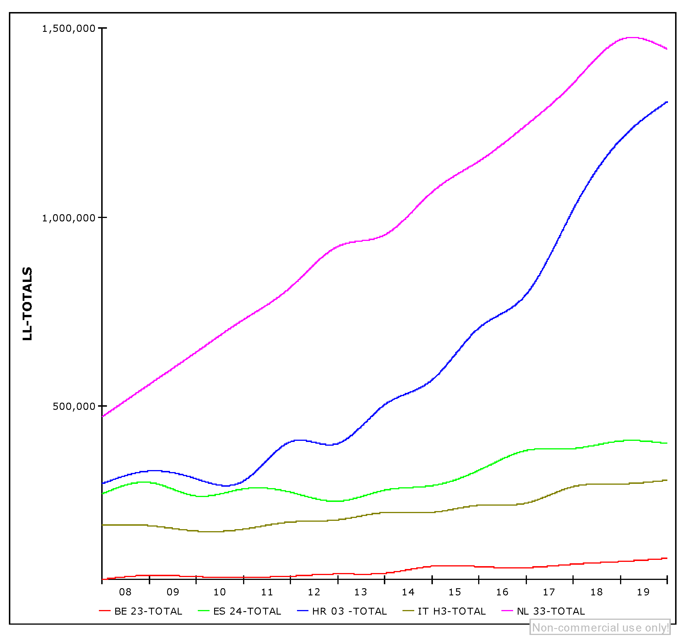
GRAPHCURVE uses linear asymptotes constructed as lines connecting two outermost fixpoints (www.powersim.com, accessed on 15 December 2020). Figure 3 describes the behavior of a GRAPHCURVE function for each Living Lab (based on its correspondent LAUs’ visitor arrivals (Table 1). Based on the GRAPHCURVE function, we calculated the annual average of the arrivals growth rates. Since we have been observing the multi-year lifecycle of a specific tourist area, we omitted seasonality analysis. The GRAPHCURVE function can also be used to validate the TALC system dynamics’ model.
As seen in Figure 3, in the observed period (2007–2019) the number of visitors at each Living Lab recorded a wavy growth. Each of the waves, i.e., the sigmoid S-shape of the curve at a specific multi-year interval, can be viewed as a distinct mini TALC. These are the destination’s short-term ‘ups and downs’, which cumulatively contribute to the shape of its long-term life cycle. Precisely, based on the cumulative effects, a specific trend of the entire Living Lab (destination) development can be predicted (as shown in Figure 3).
In his seminal paper Butler [15] dealt with six TALC stages while some other authors [52,53,54,55] were suggesting destination can pass less than six stages. Here, we propose an analytical procedure for determining the limits of different TALC stages, assuming there are three stages, i.e.,
- The supply-dominance stage;
- The demand-dominance stage;
- The restructuring stage.
5.2. Generic Structures of the TALC Model Behavior
The change of an object speed depends on its acceleration and the time needed to achieve it. The larger is the difference between the current and the desired values, the stronger is the effort to equalize them. If we deal with the inert (sluggish) system, a small change can easily become bigger and ultimately lead to unwanted consequences (the butterfly effect). However, the type and intensity of the adverse impacts depend on a system’s ability and resilience. Given this, we first have to elaborate generic structures that characterize specific patterns of behavior, such as (+)FBL delineating exponential growth, i.e., ability and (−)FBL delineating logarithmic growth. (−)FBL explains the observed variable tendency to reach a maximum, which leads to overall system resilience.
By combining these two generic structures, we reach the limits of growth, being an archetype of system dynamics whose behavior corresponds to the TALC curve behavior. Proper knowledge of the supply and demand subsystems can help to formalize this approach. By understanding how they behave, we can simulate the destination system’s responses while searching for a new state of stability.
Looking at the structural diagram in Figure 1, we can see that two feedback circuits exist in the TALC logistic curve, i.e., positive (+)FBL1 and negative (−)FBL2, showing characteristic (generic) patterns of behavior, as shown in Figure 4 and Figure 5.
In both, Figure 4 and Figure 5, the growth rate (k) is constant, and the blue curve indicates the official data on visitors for the Croatian Living Lab, consisting of seven LAUs (expressed as HR-03-Total).
(+)FBL1 describes the structure of the exponential growth pattern (Figure 4) similar to a compound interest account, where the principal is accrued based on the interest rate. Then, in the next stage, the interest rate is added to the principal, with the procedure repeated for each subsequent period. Thus, as regards the (+)FBL1, there are no limits of growth, but instead, growth depends on the penetration coefficient k and the initial state of the number of visitors V(t1).
The number of visitors V(t) can grow continuously towards infinity because there are no boundaries/limits to slow the growth. This explained, it can be concluded that (+)FBL1 describes an unlimited demand market, i.e., a situation with no competitors or any other external influence. In such a case, demand would grow exponentially with the coefficient k, according to the structure (+)FBL1.
However, the limits of growth exist and are conditioned by supply, i.e., greater demand cannot be reached out unless enabled by supply, which means that the maximum expected number of visitors (M) equals total supply. Being constant, supply may represent a constraint on expected demand with a constant penetration coefficient k. With this regard, the dynamics of the maximum expected number of visitors (M) is determined by (−)FBL2 structure that has a pattern of goal seeker (Figure 5).
The pattern of behavior between the two elaborated structures (+)FBL1 and (−)FBL2 is shown in Figure 6.
We see that the behavior pattern of the TALC logistic curve has a sigmoidal shape. In this case, k and M are constant. The growth rate acceleration occurs until the threshold point, affecting various pressures in a destination. In that point, called the inflexion point, the TALC curve changes from a convex to a concave shape.
With this regards the point of inflexion may be equated with the destination’s carrying capacity, defined as the maximum number of people who can visit a tourist destination at the same time, without causing unacceptable disturbances of the physical, economic and socio-cultural environment and reduction in visitor satisfaction [44].
Following the UNWTO’s [16] carrying capacity definition, both supply and demand subsystems have their growth thresholds. Hence, the physical, economic and socio-cultural environment (i.e., assets), impose the supply subsystem boundaries. On the other hand, the demand subsystem threshold is over if visitor satisfaction is reduced, indicating the gap between their expectations and what promised. After some time, a failure to deliver the promised offer will affect a decrease in arrivals to a destination for the sake of other competitive destinations. Opposite to this, improvements in any said environment can increase the destination’s carrying capacity, eventually attracting visitors from competitive destinations.
As soon as a destination reaches its carrying capacities, suppliers start to compete by lowering prices, cutting costs, finally resulting in an overall quality decline. Eventually, demand overpowers supply. However, absolute numbers of arrivals are growing but with diminishing growth rates. Further growth increases additional pressures until reaching a saturation threshold after which, as presumed by the TALC approach, in the last stage different scenarios may occur, depending on a destination’s resilience.
Reaching the point of inflexion provides a signal that unacceptable changes have been occurring in a destination. Moreover, the flow of the best-fit straight line describing the acceleration/deceleration of the arrivals growth rate during the observed period will enable management of the entire destination system.
In line with the above, we have decided to use the number of arrivals, as suggested by the UNWTO [16], as an indicator of the dynamics of carrying capacities and the flow function V(t) to determine the TALC stages.
To determine the saturation point, i.e., the maximum of the function V(t), it is necessary to equate its first-order derivative V′(t) with zero. The inflexion point of the function V(t) is reached by equating its second-order derivative V″(t) with zero. The value of the argument t will represent the time point at which V(t) reaches an inflexion point. The same is on the graph of the function V(t) and its first-order derivative Growth (t) and the second-order derivative Deriv2(t) (Figure 1). The simulated TALC curve has an inflexion point, i.e., Deriv2 (t) = 0 in 2010, while the moment of saturation Growth(t)à0 is expected in 2021.
Precisely, the two points of time can be considered as limits of the three TALC stages. In the first stage, there is supply-dominance, with supply-driven innovations pushing the destination’s attractiveness, eventually affecting further demand growth. In this period, supply-driven development positively affects destination, especially in terms of socio-economic and cultural impacts. This period of growth lasts until the first point of time (t-point of inflexion).
In the second stage, suppliers fiercely compete for the limited amount of resources to attract visitors. The visitors benefit from this competition and growingly visit a destination, thus indicating the demand dominance stage. Along with the growth of arrivals, many pressures are generated, indicating a destination’s maturity. Each effort to increase visitors in this stage ends up with an increase in the consumption of resources. Such an approach questions the very survival of a destination as a system. This stage begins with the inflexion point and ends up with the saturation point, indicating the maximum number of visitors.
As soon as the saturation point is achieved, the third stage can start, aiming at a destination’s restructuring, which may initiate its new development cycle together with its gravitating area or a complete decline.
Following the above explanation, it is necessary to approximate TALC as accurately as possible with real data. As presented in Figure 6, the approximate visitor curve V(t) only roughly determines the trend. The reason is that the k-coefficient of penetration together with the M-maximum expected number of visitors is constant. Following Figure 4, coefficient k determines the demand itself and its growth rate. Therefore, based on the idea of an unlimited market, we can assume that it synthesizes all elements affecting demand, thus indicating behavior according to the exponential growth pattern. Demand constraints are caused, among other things, by the attractiveness of supply—M (proxied by the maximum expected number of arrivals). Simply said, a new product in a destination can increase M. This scenario is presented in the graph of the HR-03 Total visitors’ arrival function in Figure 6. Each short-time TALC ends with a shift of the M limit, eventually initiating a new short-time TALC.
In line with the above, we can say that M synthesizes all elements of supply. If M does not grow, the function of arrivals will eventually behave according to the target search pattern, as in Figure 4. However, if the new supply is created to fight market saturation, the growth of the variable M will behave following the TALC curve. An extreme case of a structure when practically all supply was defined at the beginning of the observed period is presented by graph V(t) for the Living Lab NL-33, as shown in Figure 3.
Given the above, we can look at k and M as time-dependent variables. Thus, instead of presenting the TALC structure like in Figure 1, we can show it in Figure 7.
Dependence of the number of visitors V on variables k and M can be explained by the scenario analysis presented on Figure 8.
As presented on the left side of Figure 8, an increase of the penetration coefficient k (with a constant M) affects the demand growth rate. It does not increase the supply. Namely, lower positioned graphs have lower values of coefficient k and react more slowly to supply use. While tending to reach the offer, the top positioned graph slows down the growth of arrivals. On the right side of Figure 8, the situation with M is the opposite. Higher values of M (with a constant k) allow for an increase in the number of arrivals. Since M is easily reached with a given k, the number of arrivals with a small M (the lowest positioned graph) has a sigmoid shape. However, a high value of M takes longer to reach the supply as the number of visitors grows exponentially.
After the TALC curve crosses the inflexion point with different pressures evidenced, it is necessary to consider introducing cultural or other innovative destination products (to increase M). In the previous subsection, we have shown how to extend the observation of dynamics to a deeper level than the TALC logistic curve. The dynamization of k(t) as a representative of demand, and M(t) as a representative of supply, will enable the observation of the relationship between supply and demand over time through V(t), which characterises the life cycle of the destination.
5.3. The TALC System Dynamics Model in Powersim Studio
To develop a quantitative model following the previously described structure (Figure 8), the Powersim simulation modeling software package was used. Powersim as well as system dynamics recognizes four basic types of parameters:
- State variables—which accumulate change. It takes one moment to read them. These variables remember values and are denoted by the rectangle symbol (in Figure 9, these are k, M, SumSTDError and V-simulation Data).
- Rate variables—which indicate change, i.e., speed (first-order derivative). It takes two time moments to calculate their values. They are marked with a picture of the valve and flow. A bubble at the beginning or end indicates the source and abyss of the stream. Input or output presents a parameter for state variables. In Figure 9, these are Growth k, Growth M, Growth V, STDError.
- Auxiliary variables—which are used to clarify calculations and flow within the model. Linking them to/from rate variables enables a partial calculus. Constants are permanent identifiers throughout the simulation period. They are denoted by a rhombus (in Figure 9, k-rate, M-rate, M0, id-LAU-whose value in the model is selected based on the radio-button and the variable).
As previously described, in Figure 3, we have shown graphs of approximated visitor arrival functions for each Living Lab, based on time-series data from 2007 to 2019 (Table 1). In the next step, based on the simulation model shown in Figure 9 (which is leaning on the structure described in Figure 7), we describe graphs of the visitor arrivals’ trends. The input variables are k-rate, M-rate, and M0. By using the optimization tool in Powersim, the optimal values of the above input variables were determined to minimize the sum of standard deviations at each time point, i.e., the minimum (SumSTDError). Simply put, the optimization task is to determine the optimal values of the input variables so that the graph of the simulated number of arrivals deviates as little as possible from the graph of the approximate function based on the actual time series data collected at the level of five Living Labs (Table 1).
5.4. Scenario Analysis Based on the TALC System Dynamics Model
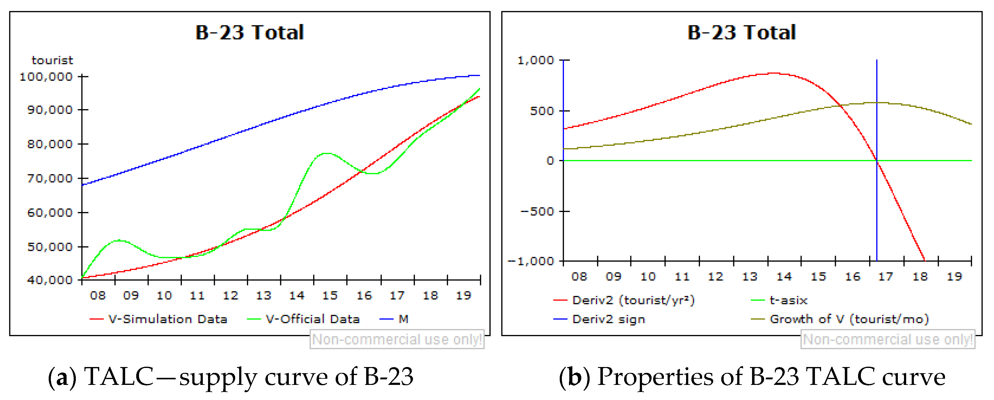
The results for each of the Living Labs/destinations are presented in Figure 10, Figure 11, Figure 12, Figure 13 and Figure 14, each one consisting of the two parts. The first part delineates the TALC curve based on the number of visitor arrivals and the second one describes the properties of the TALC curve (1st and 2nd order derivative), indicating what stage of its life cycle LL/destination is in.
Hence, the first part in each of the following figures (from Figure 10a, Figure 11a, Figure 12a, Figure 13a, Figure 14a) contains the following graphs:
- V-simulation data (red graph)—representing the number of arrivals per year, representing the trend of the observed period;
- V-Official Data (light green graph)—representing the number of arrivals per year, based on the interpolated data;
- Maximum expected number of visitors (M) (blue graph) equals total supply.
The second part in each of the following figures (from Figure 10b, Figure 11b, Figure 12b, Figure 13b, Figure 14b) contains the following graphs:
- Growth of V (dark green graph)—the first-order derivative of the V-simulation function;
- Derivative2 (red graph)—the second-order derivative of the V-simulation function;
- Derivative2 sign (blue graph)—a sign of the second-order derivative indicating moment when a destination passes from one stage to another;
- t-asix (light green graph)—drawn to enable monitoring of the first and second-order derivative functions flow.
The simulated visitor arrival curves (V-simulation data) have a sigmoidal shape corresponding to the theoretical TALC curve. Observed differences across Living Labs can be explained by different dynamics of their supply (offer) development proxied by the maximum expected number of visitors (M).
Given the above, the models are presented as follows in Figure 10:
Due to the supply expansion, at the end of the observed period (2019), the Living Lab B-23 (BELGIUM/Prov. Oost-Vlaanderen/the Scheldeland region/Denderleeuw, Willebroek) has hosted approximately 40,000 more visitors than at its beginning (in 2007) (Figure 10a). It has passed through the first (growth) stage, or the supply dominance stage in 2017 and reached its carrying capacity threshold, after which has entered the second (of the three elaborated) TALC stage, i.e., the demand dominance stage. As shown in Figure 10a, the supply (M) curve has a slight S-shape indicating the LL’s involvement with tourism. Figure 10b shows that the maximum acceleration of the visitors’ growth rates (Deriv2) was achieved in 2014, with the maximum number of arrivals reached in 2017 (Deriv2 = 0), after which it began to decline. Parallel to this, the curve representing the number of visitors (V) became concave, tending to reach the threshold indicating the maximum number of visitors.
In 2019, the LL -ES24 (SPAIN/Aragón/Huesca/Ainsa, Barbastro, Benasque, Graus, Huesca, Jaca, Sariñena) has increased the number of visitors by approximately 120,000 compared to 2007 (Figure 11a). The fastest acceleration of the growth rate was achieved in 2014, after which it began to decline (Figure 11b). It has reached its carrying capacity threshold (associated with the given supply structure) in 2016 and has entered the second lifecycle stage, i.e., the demand dominance stage.
In the observed period, the number of visitors in the LL IT-H3 (ITALY/Veneto/Vicenza/Vicenza, Caldogno, Pojana Maggiore, Grumolo delle Abbadesse, Lonigo, Montagnana) has increased by approximately 120,000 visitors (Figure 12a). However, it has grown at a lower rate than in Belgium and Spain. Hence, maximum acceleration of the growth rate was achieved in 2015, and the maximum number of visitors was reached in 2018, indicating the point when LL has entered into the second TALC stage, with a diminishing number of visitors along the remaining period (Figure 12b).
At the end of the observed period (in 2019), the LL NL-33 (NETHERLANDS/Zuid-Holland/the Rotterdam Metropolitan Region/Rotterdam, Delft, Dordrecht, Molenlanden, Barendrecht, Ridderkerk, Zwijndrecht) has realised approximately 970,000 more tourists as compared to 2007. It reached the end of the second TALC stage yet in 2015, primarily due to the role of the city of Rotterdam (as presented in Table 1 and Figure 13a). Currently, the acceleration growth rate tends to zero, which means that the number of visitors will be the same each year. The second-order derivative graph (Deriv2) indicates that the acceleration of the visitors’ growth rate has changed its direction and is not declining steeply anymore. Both the first and the second-order derivative graphs tend to zero, which means that the destination (LL) approaches the third stage of its lifecycle (Figure 13b). This particular Living Lab differs from the others concerning its supply (M) remains almost constant along the observed years, indicating that NL-33 Living Lab (destination) has not significantly improved its supply.
The LL HR-03 (CROATIA/Jadranska Hrvatska/City of Split metropolitan area/Split, Trogir, Dugopolje, Solin, Klis, Kaštela, Sinj) consists of seven municipalities, out of which four coastal ones (two inscribed on the World Heritage List) currently record significant tourist flows. The three rural municipalities have recently got involved more intensively with the tourism business. However, despite the newcomers, the whole of the Split metropolitan LL has reached its carrying capacity in 2017 and is currently in its second lifecycle stage (the demand dominance stage) (Figure 14a). The sudden take-off in terms of the number of visitors (V) resulting from the enhancement of its supply attractiveness (M) happened in the period from 2013 to 2016, when it also reaches the maximum acceleration of the visitor growth rate (Deriv2) (Figure 14b). The maximum number of visitors is achieved in 2017, meaning that it was just one-year distance between reaching the maximum acceleration of the visitor growth rate and the maximum number of visitors (arrivals).
By declining along the second stage of its lifecycle, the visitor number growth tends to reach its predefined supply M. The LL HR-03 has the steepest decline of the growth rate compared to other LLs, which means the fastest deceleration of the number of visitors. Worth noting is that HR-03 LL has accomplished the most significant advancement of its supply in the observed period, delineated by more than a million arrivals.
6. Discussion and Conclusive Remarks
Apart from the theoretical contributions, the model developed in this research has been tested and verified on five specific cases. The analysis revealed that all observed Living Labs (destinations) reached the second lifecycle stage (demand-dominance stage), with the LL NL 33-Netherlands entered as early as in 2015, and LL ITH3-Italy in 2018 (Table 2).
Considering data availability and Butler’s [15] original idea, in this model the number of visitors V is taken as the reference point, with the logistic curve explaining the destination’s development over time. The visitor growth rate acceleration occurs until the threshold point when various pressures in a destination become evident. At that point, called the inflexion point, a destination reaches its carrying capacity and enters into the so-called demand-dominance stage (corresponding to the Butler’s consolidation stage), with the TALC curve changing from a convex to a concave shape. The steeper is the decline of the growth rate, the faster is deceleration/fall of the number of visitors, as in the LL HR-03- CROATIA.
However, when interpreting the specific TALC curve behavior, it has to be borne in mind that each of the observed destinations consists of several municipalities, each one differing from another in terms of quantity and quality of resources and overall development framework. These specificities potentially affect their position on a life cycle curve and the duration of a stage they reached. Moreover, comparing peripheral/rural municipalities with the urban ones regarding tourism intensity, it becomes evident that their smallness, remoteness and overall fragility may affect reaching the carrying capacity threshold sooner than urban destinations and with fewer tourists. Given the above, we may conclude that the elaborated TALC system dynamics model cannot explain the causes affecting either demand or supply behavior. However, understanding the socio-economic framework and the trends in an observed period can help us understand the reasons behind their behavior.
The period we have chosen to observe (2007 to 2019) is specific as it encompasses the year before the global economic crisis (2007), together with the immediate recovery and the post-recovery period. Many authors [34,56,57,58] discussed the role of tourism in the period after the crisis, considering it as a means by which the capitalist system as a whole sustains itself. With this regards, they conclude that tourism was used as one of the most common responses to the 2008 global economic crisis, which is why many governments strongly stimulated it to enhance economic recovery [57]. It certainly contributed to the expansion of demand worldwide. Apart from this, the rise of low-budget airlines, social media and Internet platforms and improved living standards in highly populated countries have also led to the enormous expansion of tourism demand, leading to overtourism, especially in cities rich with cultural heritage. This trend is also evident in some of the towns belonging to the analysed Living Labs, such as Rotterdam, Split, Vicenza, and Trogir, which recorded significant demand growth in a short period. Due to them, their corresponding LLs entered the demand-dominance stage before the COVID-19 pandemic crisis.
As explained, the demand-dominance stage begins with the inflexion point ending up with the saturation point (Butler’s stagnation stage), indicating the maximum number of visitors that a destination can withstand. As soon as the saturation point is achieved, the third stage starts, when a destination’s managers have to decide which of the following strategies they should apply:
- To reduce the number of arrivals;
- To remain in the steady-state (the same number of arrivals each year), or
- To initiate a new lifecycle by introducing innovative and sustainable tourism products to enhance offer (M) and to rejuvenate destination.
The destination rejuvenation strategies and policies have been researched by many authors, such as Faulkner [59], Faulkner and Tideswell [60], Hovinen [61], Albaladejo and Martinez [62], Ferreira and Hunter [63], Malcolm-Davies [64], and many others, proving the rule of the thumb that ‘the same policy does not fit all.
Our findings have both theoretical and empirical implications.
From the theoretical standpoint, system thinking contributed to understanding the complexity and structure of a tourist destination as a system. Moreover, the system dynamics applied to modeling tourist destination life cycle (TALC) contributed to understanding its behavior and the ways information feedback governs using feedback loops, delays and stocks and flows. Worth noting is that this research added to the existing body of knowledge on the chaos and complexity concepts in researching tourism and tourist destination, which, as indicated by Olmedo and Mateos [4] and Sedarati et al. [7], is still in its initial phase. We also tried to introduce some novelty into the usual TALC modeling performed so far. To this end, we investigated the dynamics of the variables usually taken as constants, representing quite a challenging approach rarely applied, as in Lundtorp and Wanhill [65]. Unlike the original TALC model [15], suggesting six lifecycle stages, this research offered a model with three lifecycle stages, i.e., the supply-dominance stage, the demand-dominance stage, and the restructuring stage. The supply-dominance corresponds to the three stages of Butler’s model, i.e., exploration, involvement, and development stages, while the demand-dominance corresponds to Butler’s consolidation stage. Finally, the demand-dominance stage ends up with a saturation point, after which the third stage begins, e.g., the restructuring or Butler’s rejuvenation stage.
The TALC system dynamics model was performed in several phases. First, by using empirical data on visitors in five LLs from 2007 to 2019, we have shown graphs of approximated visitor arrivals functions for each Living Lab. In the next step, following a causal loop diagram of the TALC model structure, describing the interaction among the variables, the simulation model was developed using the Powersim simulation modeling software. It aimed to determine the optimal values of the input variables. Then we simulated the function of arrivals, using the graph slightly deviating from the approximated one, based on the actual time-series data on arrivals. Finally, scenario analysis based on the TALC system dynamics model, consisting of the two parts, was performed for each Living Lab. The first part delineates the TALC curve based on the number of visitor arrivals, while the second describes the properties of the TALC curve (1st and 2nd order derivative), indicating the stage of a destination/LL life cycle.
From the empirical standpoint, the above-elaborated model may be used by destination managers as a warning tool, indicating two crucial moments of a destination development cycle, i.e., the moment when it reaches its carrying capacities and the moment of saturation, after which an innovative cycle ought to begin. Using this tool, managers may timely apply appropriate strategies and policies to enhance the destination’s sustainability and prevent its decline.
Of course, this model, as any, has gaps. The main gap is associated with its inability to indicate threshold and saturation points before the accumulated problems cause stagnation and decline. Furthermore, the model is based on just one variable, i.e., the number of visitors to a destination. Additionally, it delineates only three lifecycle stages, which, of course, simplified its construction. However, by introducing more, a destination’s development path can be better understood and managed.
Given the above, future research may go in several directions.
First, based on the elaborated methodological considerations and obtained results, it may focus on introducing the third-order derivative into the TALC model, implying the moment in which the second-order derivative reaches its maximum. However, it has to be carefully considered given the inertia of a large destination system on one side and the fast changes in small destination systems on the other side, hence questioning its applicability. Namely, large systems react slowly to changes, especially to small changes characterized by the third-order derivative. On the other hand, small systems are too volatile, which brings their credibility into question. In other words, the changes of the third-order derivative characteristics can be temporary and can lead to wrong decisions. Nevertheless, investigating its applicability can enable splitting the three TALC stages into more.
In addition, by investigating specific destinations, we may learn what particular policies should be introduced to either increase, adjust, or reduce the supply, thus ending with the adjusted M (maximum expected number of visitors).
Furthermore, by introducing new variables on the supply side, a detailed simulation macro-model may be developed and used as a prognostic tool for tourist destinations, eventually supporting better decision-making.
Author Contributions
Conceptualization, M.H. and L.P.; methodology, M.H. and L.P.; software, M.H.; validation, M.H. and L.P.; formal analysis, M.H.; investigation, M.H. and L.P.; resources, M.H.; data curation, M.H.; writing—original draft preparation, M.H. and L.P.; writing—review and editing, L.P. and M.H.; visualization, M.H.; supervision, L.P.; project administration, L.P.; funding acquisition, L.P. All authors have read and agreed to the published version of the manuscript.
Funding
This article is based on research done in the context of the SmartCulTour project that has received funding from the European Union’s Horizon 2020 Research and Innovation Programme under grant agreement no. 870708. The authors of the article are solely responsible for the information, denominations and opinions contained in it, which do not necessarily express the point of view of all the project partners and do not commit them.
Institutional Review Board Statement
Not applicable.
Informed Consent Statement
Not applicable.
Data Availability Statement
Not applicable.
Conflicts of Interest
The authors declare no conflict of interest. The funders had no role in the design of the study; in the collection, analyses, or interpretation of data; in the writing of the manuscript, or in the decision to publish the results.
References
- McDonald, J.R. Complexity science: An alternative world view for understanding sustainable tourism development. J. Sustain. Tour. 2009, 17, 455–471. [Google Scholar] [CrossRef]
- Farrell, B.H.; Twining-Ward, L. Reconceptualizing tourism. Ann. Tour. Res. 2004, 31, 274–295. [Google Scholar] [CrossRef]
- Baggio, R. Symptoms of Complexity in a Tourism System. Tour. Anal. 2008, 13, 1–20. [Google Scholar] [CrossRef] [Green Version]
- Olmedo, E.; Mateos, R. Quantitative characterization of chaordic tourist destination. Tour. Man. 2015, 47, 115–126. [Google Scholar] [CrossRef]
- Faulkner, B.; Valerio, P. Towards an integrative approach to tourism demand forecasting. Tour. Man. 1995, 16, 29–37. [Google Scholar]
- Parry, B.; Drost, R. Is chaos good for your profits? Int. J. Cont. Hosp. Man. 1995, 7, 1–3. [Google Scholar]
- Sedarati, P.; Santos, S.; Pintassilgo, P. System Dynamics in Tourism Planning and Development. Tour. Plan. Dev. 2019, 16, 256–280. [Google Scholar] [CrossRef]
- Zhang, Z.; Ding, Z.J. The Systematic Spatial Characteristics of Sports Tourism Destinations in the Core Area of Marine Economy. J. Coast. Res. 2020, 112, 109–111. [Google Scholar] [CrossRef]
- Valeri, M.; Baggio, R. Social network analysis: Organizational implications in tourism management. Int. J. Org. Anal. 2020, 29, 342–353. [Google Scholar] [CrossRef]
- Rodriguez-Giron, S.; Vanneste, D. Tourism systems thinking: Towards an integrated framework to guide the study of the tourism culture & communication. Tour. Tour. Cult. Commun. Comm. 2019, 19, 1–16. [Google Scholar] [CrossRef]
- Yang, Z.Y.; Yin, M.; Xu, J.G.; Lin, W. Spatial evolution model of tourist destinations based on complex adaptive system theory: A case study of Southern Anhui, China. J. Geogr. Sci. 2019, 29, 1411–1434. [Google Scholar] [CrossRef] [Green Version]
- Iandolo, F.; Fulco, I.; Bassano, C.; D’Amore, R. Managing a tourism destination as a viable complex system. The case of Arbatax Park. Land Use Policy 2019, 84, 21–30. [Google Scholar] [CrossRef]
- Speakman, M. Paradigm for the Twenty-first Century or Metaphorical Nonsense? The Enigma of Complexity Theory and Tourism Research. Tour. Plan. Dev. 2017, 14, 282–296. [Google Scholar] [CrossRef]
- Pizzitutti, F.; Walsh, S.J.; Rindfuss, R.R.; Gunter, R.; Quiroga, D.; Tippett, R.; Mena, C.F. Scenario planning for tourism mana-gement: A participatory and system dynamics model applied to the Galapagos Islands of Ecuador. J. Sustain. Tour. 2017, 25, 1117–1137. [Google Scholar] [CrossRef]
- Butler, R. The concept of a tourist area cycle of evolution: Implications for management of resources. Can. Geogr. 1980, 24, 5–12. [Google Scholar] [CrossRef]
- United Nations World Tourism Organization (UNWTO). Report of the Secretary General of the General Programme of Work for the Period 1980–1981: Tourist Markets, Promotion and Marketing-Saturation of Tourist Destinations; UNWTO: Madrid, Spain, 1981. [Google Scholar]
- Jere Lazanski, T.; Kljajić, M. Systems approach to complex systems modelling with special regards to tourism. Kybernetes 2006, 35, 1048–1058. [Google Scholar] [CrossRef]
- Bui, H.L.; Jones, T.E.; Weaver, D.B.; Le, A. The adaptive resilience of living cultural heritage in a tourism destination. J. Sustain. Tour. 2020, 28, 1022–1040. [Google Scholar] [CrossRef]
- Jere Jakulin, T. Systems Approach to Tourism: A Methodology for Defining Complex Tourism System. Organizacija 2017, 50, 208–215. [Google Scholar] [CrossRef] [Green Version]
- Baggio, R.; Sainaghi, R. Complex and chaotic tourism systems: Towards a quantitative approach. Int. J. Contemp. Hosp. Manag. 2011, 23, 840–861. [Google Scholar] [CrossRef]
- Baranger, M. Chaos, Complexity, and Entropy—A Physics Talk for Non-Physicists. Center for Theoretical Physics, Laboratory for Nuclear Science and Department of Physics Massachusetts Institute of Technology, Cambridge and New England Complex Systems Institute. 2010. Available online: http://grex.cyberspace.org/~jayk/ChaosComplexityAndEntropy.pdf (accessed on 15 January 2021).
- Berkes, F.; Ross, H. Panarchy and community resilience: Sustainability science and policy implications. Environ. Sci. Policy 2016, 61, 185–193. [Google Scholar] [CrossRef]
- Faulkner, B.; Russell, R. Chaos and complexity in tourism: In search of a new perspective. Pac. Tour. Rev. 1997, 1, 93–102. [Google Scholar]
- Russell, R.; Faulkner, B. Entrepreneurship, Chaos and the Tourism Area Lifecycle. Ann. Tour. Res. 2004, 31, 556–579. [Google Scholar] [CrossRef]
- Petrić, L. Has the myth of tourist destination sustainability faded? Behind the curtains of the global crises. In Proceedings of the 2nd International Scientific Conference “Tourism in Southern and Eastern Europe”, Opatija, Croatia, 15–18 May 2013; Janković, S., Smolčić Jurdana, D., Eds.; Faculty of Tourism and Hospitality Management: Opatija, Croatia, 2013; pp. 19–23. [Google Scholar]
- McKercher, B. A Chaos Approach to Tourism. Tour. Manag. 1999, 20, 425–434. [Google Scholar] [CrossRef]
- Williams, B.K.; Szaro, R.C.; Shapiro, C.D. Adaptive Management: The US Department of the Interior Technical Guide; Adaptive Management Working Group, US Department of the Interior: Washington, DC, USA, 2007. Available online: https://www.doi.gov/sites/doi.gov/files/migrated/ppa/upload/TechGuide.pdf (accessed on 7 April 2021).
- Murphy, P. Tourism: A Community Approach; Methuen: New York, NY, USA, 1985. [Google Scholar]
- Tosun, C. Limits to community participation in the tourism development process in developing countries. Tour. Manag. 2000, 21, 613–633. [Google Scholar] [CrossRef] [Green Version]
- Tosun, C.; Timothy, D.J. Arguments for community participation in tourism development. Tour. Stud. 2003, 14, 2–11. [Google Scholar]
- Beeton, S. Community Development through Tourism; Landlink Press: Collingwood, Australia, 2006. [Google Scholar]
- Eyisi, A.; Lee, D.; Trees, K. Facilitating collaboration and community participation in tourism development: The case of South-Eastern Nigeria. Tour. Hosp. Res. 2020. [Google Scholar] [CrossRef]
- Rasoolimanesh, S.M.; Jaafar, M.; Kock, N.; Ahmad, A.G. The effects of community factors on residents’ perceptions toward World Heritage Site inscription and sustainable tourism development. J. Sustain. Tour. 2017, 25, 198–216. [Google Scholar] [CrossRef]
- Higgins-Desbiolles, F.; Carnicelli, S.; Krolikowski, C.; Wijesinghe, G.; Boluk, K. Degrowing tourism: Rethinking tourism. J. Sustain. Tour. 2019, 27, 1926–1944. [Google Scholar] [CrossRef]
- Butowski, L. Sustainable Tourism: A Human-Centered Approach. Sustainability 2021, 13, 1835. [Google Scholar] [CrossRef]
- Miller, D.S.; Gonzalez, C.; Hutter, M. Phoenix tourism within dark tourism. Worldw. Hosp. Tour. Themes 2017, 9, 196–215. [Google Scholar] [CrossRef]
- Butler, R. The Origins of the Tourism Area Life Cycle. In The Tourism Area Life Cycle, Applications and Modifications; Butler, R., Ed.; Channel View Publications: Clevedon, UK, 2006; Volume 1, pp. 13–26. [Google Scholar]
- Coyle, G. System Dynamics Modelling: A Practical Approach; Springer-Science+Business Media: Berlin, Germany, 1996. [Google Scholar]
- Ogata, K. Modern Control Engineering Systems, 3rd ed.; Prentice Hall: Hoboken, NJ, USA, 1997. [Google Scholar]
- Forrester, J.W. Urban Dynamics; M.I.T. Press: Cambridge, MA, USA, 1969; p. xiv + 290. [Google Scholar]
- Sterman, J.D. System Dynamics: Systems Thinking and Modelling for a Complex World; Engineering Systems Division Working Paper Series; Massachusetts Institute of Technology: Cambridge, MA, USA, 2002; Available online: https://dspace.mit.edu/bitstream/handle/1721.1/102741/esd-wp-2003-01.13.pdf?sequence=1&isAllowed=y (accessed on 3 February 2021).
- Davidsen, P. The structure±behavior diagram: Understanding the relationship between structure and behavior in complex dynamic systems. In Proceedings of the System Dynamics Conference, Utrecht, The Netherlands, 14–17 July 1992; Vennis, J.A.M., Ed.; The Systems Dynamics Society: Albany, NY, USA, 1992; pp. 127–140. [Google Scholar]
- Forrester, J.W. Industrial Dynamics; The Massachusetts Institute of Technology: Cambridge, MA, USA, 1961. [Google Scholar]
- Rahmandad, H.; Repenning, N.; Sterman, J. Effects of feedback delay on learning. Syst. Dyn. Rev. 2009, 25, 309–338. [Google Scholar] [CrossRef]
- Huang, J.B. Analytical and Computational Methods for Analyzing Feedback Structure in System Dynamics Models. Ph.D. Thesis, School of Engineering & Informatics, National University of Ireland, Galway, Ireland, 7 October 2012. [Google Scholar]
- Richardson, G.P. Feedback Thought in Social Science and Systems Theory; University of Pennsylvania Press: Philadelphia, PA, USA, 1991. [Google Scholar]
- Richardson, G.P. Loop polarity, loop dominance, and the concept of dominant polarity. Syst. Dyn. Rev. 1995, 11, 67–88. [Google Scholar] [CrossRef]
- Ford, F.A. Modeling the Environment: An Introduction to System Dynamics Models of Environmental Systems; Island Press: Washington, DC, USA, 1999. [Google Scholar]
- Pejić-Bach, M.; Čerić, V. Developing System Dynamics Models with Step by Step approach. J. Inf. Organ. Sci. 2007, 31, 171–185. [Google Scholar]
- Cole, S. Synergy and congestion in the tourist destination life cycle. Tour. Manag. 2012, 33, 1128–1140. [Google Scholar] [CrossRef]
- Petrić, L.; Škrabić Perić, B.; Hell, M.; Kuliš, Z.; Mandić, A.; Pivčević, S.; Šimundić, B.; Muštra, V.; Grgić, J.; Mikulić, D. Report outlining the SRT framework. Deliverable 4.2. of the Horizon 2020 project SmartCulTour (GA number 870708). Published on the Project Web Site on February 2021. Available online: http://www.smartcultour.eu/deliverables/ (accessed on 3 March 2021).
- Haywood, K.M. Can the tourist area life-cycle be made operational? Tour. Manag. 1986, 7, 154–167. [Google Scholar] [CrossRef]
- Dealbuquerque, K.; Mcelroy, J.L. Caribbean small-island tourism styles and sustainable strategies. Environ. Manag. 1992, 16, 619–632. [Google Scholar] [CrossRef]
- Prideaux, B. The resort development spectrum—A new approach to modelling resort development. Tour. Manag. 2000, 21, 225–240. [Google Scholar] [CrossRef]
- Romao, J.; Guerreiro, J.; Rodrigues, P. Regional tourism development: Culture, nature, life cycle and attractiveness. Curr. Issues Tour. 2013, 16, 517–534. [Google Scholar] [CrossRef]
- Fletcher, R. Sustaining Tourism, Sustaining Capitalism? The Tourism Industry’s Role in Global Capitalist Expansion. Tour. Geogr. 2011, 13, 443–461. [Google Scholar] [CrossRef]
- Fletcher, R.; Murray Mas, I.; Blanco-Romero, A.; Blázquez-Salomet, M. Tourism and de-growth: An emerging agenda for research and praxis. J. Sustain. Tour. 2019, 10, 1–19. [Google Scholar] [CrossRef]
- Seyfi, S.; Hall, C.M. COVID-19 pandemic, tourism and de-growth. In De-Growth and Tourism: New Perspectives on Tourism Entrepreneurship, Destinations and Policy; Hall, C.M., Lundmark, L., Zhang, J., Eds.; Routledge: London, UK, 2021; pp. 287–313. [Google Scholar]
- Faulkner, B. Rejuvenating a Maturing Tourist Destination: The Case of the Gold Coast; Common Ground Publishing Pty Ltd.: Melbourne, Australia, 2002; Available online: https://citeseerx.ist.psu.edu/viewdoc/download?doi=10.1.1.505.3592&rep=rep1&type=pdf (accessed on 7 April 2021).
- Faulkner, B.; Tideswell, C. Rejuvenation a Maturing Tourist Destination; The case of the Gold Coast, Australia. In The Tourism Area Life Cycle, Applications and Modifications; Butler, R., Ed.; Channel View Publications: Clevedon, UK, 2006; Volume 1, pp. 306–335. [Google Scholar]
- Hovinen, G.R. Lancaster County, the TALC and the search for sustainable tourism. In The Tourism Area Life Cycle, Applications and Modifications; Butler, R., Ed.; Channel View Publications: Clevedon, UK, 2006; Volume 1, pp. 73–90. [Google Scholar]
- Albaladejo, I.; Martinez Garcia, M.P. The post-stagnation stage for mature tourism areas: A mathematical modelling process. Tour. Econ. 2017, 2, 387–402. [Google Scholar] [CrossRef]
- Ferreira, S.L.A.; Hunter, C.A. Wine tourism development in South Africa: A geographical analysis. Tour. Geogr. 2017, 19, 676–698. [Google Scholar] [CrossRef]
- Malcom-Davies, J. The TALC for Heritage Sites. In The Tourism Area Life Cycle, Applications and Modifications; Butler, R., Ed.; Channel View Publications: Clevedon, UK, 2006; Volume 1, pp. 162–180. [Google Scholar]
- Lundtorp, S.; Wanhill, S. The resort lifecycle theory. Generating Processes and Estimation. Ann. Tour. Res. 2001, 28, 947–964. [Google Scholar] [CrossRef]
Figure 1.
Casual loop diagram of the TALC model.

Figure 2.
Basic concept of calculation.

Figure 3.
Behavior of a GRAPHCURVE function for all Living Labs.

Figure 4.
Exponential growth.

Figure 5.
Goal seeking.

Figure 6.
Pattern of behavior and graphs of the first and second order derivative of the TALC logistic curve.
Figure 6.
Pattern of behavior and graphs of the first and second order derivative of the TALC logistic curve.

Figure 7.
Casual loop diagram of the TALC model in the context of supply-demand dynamics.

Figure 8.
Dependence of the number of visitors V on variables k and M.

Figure 9.
Flow diagram of the HR 03-LL TALC model simulation presented by Powersim symbols.

Figure 10.
TALC—supply curve and properties of B-23.

Figure 11.
TALC—supply curve and properties of ES-24.

Figure 12.
TALC—supply curve and properties of IT-H3.

Figure 13.
TALC—supply curve and properties of NL-33.

Figure 14.
TALC—supply curve and properties of HR-03.


Table 1.
Data on arrivals along the LAUs and LLs in the period from 2007–2019. Source: [51].
Table 1.
Data on arrivals along the LAUs and LLs in the period from 2007–2019. Source: [51].
| 2007 | 2008 | 2009 | 2010 | 2011 | 2012 | 2013 | 2014 | 2015 | 2016 | 2017 | 2018 | 2019 | |
|---|---|---|---|---|---|---|---|---|---|---|---|---|---|
| BE 23-TOTAL | 40,727 | 51,614 | 47,882 | 46,696 | 49,077 | 55,170 | 56,907 | 75,382 | 74,473 | 71,756 | 80,759 | 88,008 | 96,358 |
| Bornem | 12,020 | 12,105 | 11,889 | 12,146 | 12,543 | 12,325 | 12,003 | 13,315 | 13,700 | 13,356 | 13,876 | 13,601 | 15,660 |
| Pu.-Si.-Am. | 2638 | 2996 | 3354 | 3713 | 4071 | 4429 | 4787 | 5442 | 5395 | 6144 | 5276 | 6570 | 7418 |
| Aalst | 18,759 | 28,618 | 25,143 | 23,230 | 25,405 | 29,688 | 31,119 | 48,224 | 47,814 | 44,537 | 52,851 | 58,623 | 62,628 |
| Berlare | 2838 | 2839 | 2487 | 2797 | 2606 | 3151 | 2482 | 2100 | 2862 | 2732 | 2921 | 3109 | 4020 |
| Dendermonde | 4472 | 5056 | 5009 | 4810 | 4452 | 5577 | 6516 | 6301 | 4702 | 4987 | 5835 | 6105 | 6632 |
| ES 24-TOTAL | 267,090 | 297,506 | 261,463 | 280,208 | 271,409 | 247,693 | 276,771 | 288,902 | 329,622 | 381,897 | 387,165 | 407,220 | 400,611 |
| Ainsa | 3439 | 6356 | 9273 | 12,190 | 15,107 | 18,024 | 19,426 | 26,888 | 25,260 | 29,692 | 32,609 | 55,503 | 35,258 |
| Benasque | 70,753 | 68,201 | 63,243 | 72,698 | 67,585 | 49,759 | 56,079 | 57,041 | 59,285 | 71,142 | 81,818 | 78,271 | 79,695 |
| Huesca | 77,565 | 92,458 | 71,568 | 69,988 | 66,990 | 65,409 | 72,650 | 78,374 | 90,168 | 92,857 | 90,091 | 90,091 | 90,168 |
| Jaca | 115,333 | 130,491 | 117,379 | 125,332 | 121,727 | 114,501 | 128,616 | 126,599 | 154,909 | 188,206 | 182,647 | 183,355 | 195,490 |
| HR 03-TOTAL | 294,370 | 327,557 | 306,968 | 301,086 | 405,275 | 400,456 | 503,400 | 568,271 | 706,592 | 794,964 | 1,019,852 | 1,204,130 | 1,305,993 |
| Dugopolje | 3000 | 4000 | 9000 | 10,282 | 29,676 | 32,258 | 61,193 | 46,726 | 53,960 | 25,927 | 51,299 | 49,159 | 45,779 |
| Kaštela | 28,501 | 29,987 | 26,893 | 25,509 | 54,880 | 32,670 | 41,016 | 42,406 | 50,191 | 60,364 | 83,605 | 100,530 | 114,990 |
| Klis | 100 | 100 | 100 | 100 | 100 | 300 | 300 | 300 | 500 | 877 | 1909 | 2931 | 4085 |
| Sinj | 8689 | 9645 | 7649 | 7179 | 7694 | 7110 | 9035 | 10,691 | 10,266 | 9633 | 11,317 | 13,116 | 11,620 |
| Solin | 2500 | 4000 | 5500 | 7530 | 14,590 | 11,118 | 6915 | 10,422 | 14,449 | 15,693 | 22,139 | 32,042 | 41,322 |
| Split | 185,718 | 211,299 | 176,185 | 203,539 | 252,287 | 265,630 | 318,057 | 381,227 | 487,474 | 583,041 | 720,325 | 859,224 | 941,185 |
| Trogir | 65,862 | 68,526 | 81,641 | 46,947 | 46,048 | 51,370 | 66,884 | 76,499 | 89,752 | 99,429 | 129,258 | 147,128 | 147,012 |
| IT H3-TOTAL | 183,858 | 183,119 | 168,631 | 173,731 | 192,618 | 198,268 | 217,598 | 218,073 | 236,852 | 242,609 | 286,103 | 293,648 | 303,550 |
| Caldogno | 1833 | 2029 | 1742 | 1651 | 1838 | 2121 | 1131 | 842 | 842 | 842 | 842 | 842 | 842 |
| Gr. delle Abb. | 1769 | 3146 | 5642 | 3663 | 8396 | 9622 | 11,115 | 11,038 | 11,748 | 12,458 | 13,168 | 13,878 | 14,588 |
| Lonigo | 7403 | 8013 | 7154 | 7136 | 6718 | 6949 | 6913 | 7130 | 7717 | 8304 | 8891 | 9478 | 10,065 |
| Montagnana | 6121 | 6369 | 4636 | 4681 | 4667 | 3700 | 4055 | 4514 | 3248 | 1982 | 716 | 0 | 0 |
| Vicenza | 166,732 | 163,562 | 149,457 | 156,600 | 170,999 | 175,876 | 194,384 | 194,549 | 213,297 | 219,023 | 262,486 | 270,000 | 279,871 |
| NL 33-TOTAL | 471,342 | 557,097 | 642,852 | 728,607 | 814,361 | 922,282 | 953,188 | 1,065,836 | 1,148,228 | 1,243,377 | 1,354,261 | 1,469,674 | 1,445,218 |
| Barendrecht | 12,801 | 14,187 | 15,573 | 16,959 | 18,345 | 19,260 | 20,924 | 22,601 | 24,012 | 25,013 | 28,755 | 28,106 | 27,980 |
| Delft | 26,527 | 29,515 | 32,503 | 35,490 | 38,478 | 40,290 | 44,185 | 48,050 | 50,688 | 52,455 | 60,653 | 59,572 | 59,501 |
| Dordrecht | 33,779 | 36,944 | 40,109 | 43,274 | 46,439 | 48,165 | 52,419 | 56,548 | 59,602 | 61,432 | 70,246 | 68,517 | 68,513 |
| Ridderkerk | 12,350 | 13,638 | 14,927 | 16,215 | 17,503 | 18,430 | 19,986 | 21,473 | 22,625 | 23,494 | 27,160 | 26,702 | 26,529 |
| Rotterdam | 373,226 | 448,964 | 524,702 | 600,440 | 676,179 | 778,000 | 796,000 | 896,000 | 969,000 | 1,058,000 | 1,141,000 | 1,261,000 | 1,237,000 |
| Zwijndrecht | 12,659 | 13,848 | 15,038 | 16,228 | 17,418 | 18,137 | 19,674 | 21,165 | 22,302 | 22,982 | 26,447 | 25,777 | 25,695 |
Table 2.
The comparative presentation of the LLs’ lifecycle stages.
| Living Lab | The Year When the Maximum Acceleration of the Visitor Growth Rate Was Reached | The Year When the Maximum Growth Rate of Arrivals Is Reached (Carrying Capacities Threshold) | Lifecycle Stage |
|---|---|---|---|
| BE-23; BELGIUM, Prov. Oost-Vlaanderen and Antwerpen, the Scheldeland region | 2014 | 2017 | The second lifecycle stage-the demand dominance stage |
| ES 24: SPAIN, Aragón, Huesca | 2014 | 2016 | The second lifecycle stage- the demand dominance stage |
| HR-03; CROATIA, City of Split metropolitan area | 2016 | 2017 | The second lifecycle stage- the demand dominance stage |
| IT H3; ITALY, Veneto, Vicenza | 2015 | 2018 | The second lifecycle stage- the demand dominance stage |
| NL 33; NETHERLANDS, Zuid-Holland, The Rotterdam Metropolitan Region | 2015 | 2015 | The end of the second lifecycle stage |
Publisher’s Note: MDPI stays neutral with regard to jurisdictional claims in published maps and institutional affiliations. |
© 2021 by the authors. Licensee MDPI, Basel, Switzerland. This article is an open access article distributed under the terms and conditions of the Creative Commons Attribution (CC BY) license (https://creativecommons.org/licenses/by/4.0/).
Share and Cite
MDPI and ACS Style
Hell, M.; Petrić, L. System Dynamics Approach to TALC Modeling. Sustainability 2021, 13, 4803. https://0-doi-org.brum.beds.ac.uk/10.3390/su13094803
AMA Style
Hell M, Petrić L. System Dynamics Approach to TALC Modeling. Sustainability. 2021; 13(9):4803. https://0-doi-org.brum.beds.ac.uk/10.3390/su13094803
Chicago/Turabian StyleHell, Marko, and Lidija Petrić. 2021. "System Dynamics Approach to TALC Modeling" Sustainability 13, no. 9: 4803. https://0-doi-org.brum.beds.ac.uk/10.3390/su13094803
Note that from the first issue of 2016, this journal uses article numbers instead of page numbers. See further details here.