
Activity Scheduling Behavior of the Visitors to an Outdoor Recreational Facility Using GPS Data


1
Toyota Central R&D Labs., Inc., Nagakute 480-1192, Japan
2
Institute of Materials and Systems for Sustainability, Nagoya University, Nagoya 464-8603, Japan
*
Author to whom correspondence should be addressed.
Sustainability 2021, 13(9), 4871; https://0-doi-org.brum.beds.ac.uk/10.3390/su13094871
Submission received: 22 March 2021
/
Revised: 15 April 2021
/
Accepted: 15 April 2021
/
Published: 26 April 2021
(This article belongs to the Special Issue Smart and Sustainable Streets)
Abstract
:Understanding the decision-making behavior of pedestrians is essential for urban designers and developers in enhancing the commercial and aesthetic value of streets and other urban spaces. However, limited research has been conducted on the activity scheduling behavior of pedestrians. The majority of the studies conducted on outdoor facilities utilize spatial representations by links and are unable to sufficiently represent the highly flexible behavior of pedestrians. This study proposes a new method to discretize data from the global positioning system (GPS) into a two-dimensional grid-based spatial representation with a high spatial resolution. The information regarding the stay at the point of interests (POIs) is extracted from the discretized data, and the activity scheduling model is estimated. The estimation results indicate that the visitors’ attributes, such as the age of the representative and number of children, affect the probability of the activity choice and the time spent at the POI. The probability of choosing the main gate increases in the latter half of the stay, confirming the existence of time pressure. The information on the decision-making behavior of the visitors to a facility, obtained from the GPS data, can be applied to the data-oriented spatial design process to create attractive and lively spaces.
1. Introduction
The research literature on urban studies reports that high-quality urban spaces deliver higher value to the users in terms of economic, social, health, and environmental factors [1]. In particular, recent empirical studies have suggested that high-quality public spaces, including streets, squares, and plazas, promote social and psychological health [2] and pose a positive impact on the well-being and liveliness [3]. Public spaces are vital as social spaces rather than being limited as channels of movement or intersections for pedestrians. Thus, the creation of attractive and lively public spaces requires an understanding of the pedestrians’ behaviors in terms of attractiveness, value and the reason for manifesting various behaviors in such spaces.
Pedestrian behavior can be categorized into the following three interrelated levels [4]:
- Strategic level (departure time choice and activity pattern choice);
- Tactical level (activity scheduling, activity area choice, and route choice);
- Operational level (direction and speed).
The development of pedestrian behavior models has been primarily focused on the operational level, which involves determining the direction and the speed of a pedestrian and interactions with other pedestrians and obstacles [5,6,7,8,9]. However, research on the higher-level decision-making behaviors is limited to exit choices in evacuation scenarios [10,11,12] and route choices within a facility [13,14]. Moreover, research on activity pattern choice and activity scheduling is limited as well.
Understanding activity scheduling is particularly important in the urban design and the development process, to increase the commercial and aesthetic value of urban spaces such as streets. The activity scheduling models can be categorized into two major types: rule-based models that determine the activities based on predetermined rules and utility maximization models that determine the activities based on the concept of utility maximization [15]. The utility maximization models are based on microeconomics and are most applicable for general activity-based models, owing to their mathematical rigor, regardless of the pedestrian models. The applications of the activity scheduling models based on the utility maximization models include nested logit-based activity-choice models [16] and dynamic activity choice models [17,18].
The activity choice of pedestrians may not be explicit. This characteristic can be observed in cases where the act of walking becomes an activity such as shopping, sightseeing, and so on [19]. This behavior is common because people make itineraries without a predetermined destination and then explore attractive places along the way [20]. One of the few attempts to describe such pedestrian behavior is a model which combines the destination choice, the route choice, and an impulse stop in an inner-city shopping area [21]. Additionally, recent studies have demonstrated that the combination of positive utility and space-time constraints can better explain the pedestrian-specific behavior such as detours and short stays in the path choice [22]. Moreover, several studies have shown that the application of dynamic models with agent effects for the activity choice outperforms the static models such as multinomial logit models [17,18]. Although these studies can determine the order of activities, they do not consider the allocation of the activity time. This study attempts to apply the dynamic activity scheduling model [23] for addressing the issue regarding pedestrian activity scheduling. Notably, the management of travel time that represents the minimum time required for allocation was challenging for the original model [23]. Therefore, the proposed model is extended to handle this minimum required time.
The widespread use of Global Positioning System (GPS) devices has enabled the collection of large amounts of tracking data, which has in turn allowed data analysis by several approaches, including understanding the travel behaviors of people [24,25] and improving mobility services [26]. This is no exception in the case of analyzing pedestrians [27,28]. Typically, pedestrian networks are not as readily available as road networks, which is another major problem in handling pedestrian activity [27]. In addition, outdoor facilities such as the ones considered in this study have open spaces, including lawn areas and plazas and it is difficult to represent these spaces with the conventional link expressions. Therefore, the proposed method adopts a spatial representation with a detailed spatial resolution grid (15 m grid per square and 10 s sampling), which allows for the representation of open spaces. Furthermore, the proposed model can be combined with sequential path choice and a grid-based spatial representation [22] to appropriately represent the aforementioned pedestrian-specific behaviors.
The contributions of this paper are as follows:
- A processing method is proposed to discretize the GPS data into a two-dimensional grid-based spatial representation with high spatial resolution in order to represent the complex behavior of pedestrians.
- The decision-making behavior of the visitors is clarified based on the activity choice and the time allocation in an outdoor facility by using the dynamic activity scheduling model.
The proposed model can be applied to the data-oriented spatial design to create attractive and lively spaces by clarifying the decision-making behavior of the visitors regarding their activity choice and the time allocation based on the GPS data.
This paper is organized as follows. Section 2 presents a literature review of the spatial representation of the GPS data and the activity scheduling models for pedestrians. The data acquisition, data processing methods, and activity scheduling model are detailed in Section 3, and the results are discussed in Section 4. Lastly, the study is summarized and the future scope is discussed in Section 5.
2. Literature Review
This section presents a literature review of the spatial representation of the GPS data and the activity scheduling models for pedestrians.
2.1. Spatial Representation of GPS Data
A recent study conducted with the GPS data of pedestrians proposed a method to simultaneously estimate the path choice model parameters for a pedestrian during estimating the various errors for each link [28]. However, the study assumed that the pedestrian networks were known. An additional study proposed a method for automatic generation of a pedestrian network using multiple GPS traces, because pedestrian networks are generally not as readily available as road networks [27]. The similarity between these studies is constituted by the usage of links representing the space; however, they cannot adequately represent the highly flexible behavior of pedestrians.
Conversely, the grid-based (or cell-based) representation is a more flexible spatial representation of the pedestrians, and several of such representations are primarily applicable for indoor usage, especially in cellular automata models [6,29,30]. Additionally, the grid-space representation was applied to a network representation for route choice models [13], development of an indoor tracking algorithm [31], and pedestrian behavior prediction for robot path planning [32]. As depicted in these models, most of the research using grid-based spatial representation has focused on indoor environments. Consequently, a pedestrian path choice model representing pedestrian detour and stay behavior was proposed for outdoor environments [22]. Although the grid-based spatial representation in this study was used as an epitome of outdoor facility, a purely numerical and virtual experiment was conducted. In the only study of grid-based spatial representation based on actual GPS data, the impact of the built environment on pedestrian and bicycle commuting trips was examined using a grid-based spatial representation with a spatial resolution of 20 m [33], wherein the GPS points were assigned to a grid containing each point, and there was no provision for assigning the points in case the noise was included.
As mentioned earlier, the grid-based spatial representation has primarily focused in indoor environments, and its application in the outdoor environments is extremely limited. In addition, a high spatial resolution and consistent trajectory information are required to obtain detailed information on the location and duration of the activities. Therefore, we propose a method to satisfy these requirements using only GPS data.
2.2. Activity Scheduling Models for Pedestrians
Research pertaining to pedestrian activity scheduling includes normative pedestrian behavior theory based on the concept of utility maximization [4], wherein the model covered route choice, activity area choice, and activity scheduling, and simultaneously optimized them through utility maximization. Another study applied a nested logit model to generate the activity schedules by dividing the activity choice at the airport into three periods: before-check-in, before-security, and before-boarding [16]. Additionally, several studies have demonstrated that the application of dynamic models for the activity choice is more representative when compared to the static models such as the multinomial logit models [17,18]. However, these studies only determined the order of the activities and did not consider the allocation of the activity time.
Although the pedestrian activity time allocation and the monetary expenditure in a city center has been modeled, the spatial elements have not been considered [34]. In this study, the dynamic activity scheduling model [23] was employed to simultaneously consider the dynamic activity choice and activity time allocation. Moreover, the dynamic activity scheduling model has been already applied to the pedestrians’ time allocation and activity-area choice [35]. Instead of using links, the model categorized the pedestrian walking patterns into activity areas with a scale of 100–300 m and employed the dynamic activity scheduling model to represent the activity-area choice and time allocation. However, the model considered the roughly divided activity areas, which varied from a model focusing on the activity choice for a specific facility. In contrast, the activity choice and activity time allocation was modeled in a facility for multiple points of interest (POIs) by using a detailed spatial representation at the 15-meter level of the resolution grid.
3. Materials and Methods
In this section, the GPS data acquisition experiment was first described. Thereafter, the proposed data processing method was described in detail. Concretely, this study proposed a processing method for discretizing GPS data with noise and missing data into a two-dimensional grid-based spatial representation with a high spatial resolution of 15 m. The information regarding the duration of stay at the POIs was extracted from the discretized data, and a dynamic activity scheduling model comprising an activity choice model and an activity time allocation model was estimated based on this information.
3.1. Data Acquisition
The facility to be analyzed in this study is the “Tango Kingdom,” which is one of the largest roadside stations in western Japan. The Tango Kingdom covers an area of roughly 34 ha. The park includes various facilities such as restaurants, go-karts, and animal spaces, making it an outdoor facility suitable for both children and adults.
The data was acquired over a total of two days from 22–23 August 2015, with the cooperation of the visitors to the Tango Kingdom. Bluetooth low-energy (BLE) transmitters and GPS loggers were distributed to the subjects and they were allowed to walk freely around the park as originally intended. A simple questionnaire was also distributed to determine the age and the gender of the representatives, the group composition, the number of visits, place of residence, and the purpose of visit. The observations were obtained from a total of 277 groups of visitors over a course of two days.
The GPS logger used in this study was the i-gotU gt-600 from Mobile Action Technology Inc., which uses the SiRF IV chipset and has a horizontal positional accuracy of 2.5 m (2D RMS). The BLE receivers were installed at a total of 12 locations in the park (Figure 3), and upon receiving a radio wave emitted by a BLE transmitter, the position, time, chassis identification number, and radio wave strength of the receiver were recorded on the server.
Based on a comparative analysis between the BLE and GPS [36], both methods acquired accurate information on the activity travel behaviors of visitors. However, the BLE signal could reach farther under certain conditions, such as large unobstructed spaces, thereby resulting in false positives and lower accuracy. The proposed method using the GPS is superior under such conditions as well as enables extraction of the stay information based on the entire trajectory, even in situations where recording observations is challenging, such as inside buildings. In the following section, the proposed data processing methods are described in detail.
3.2. Data Processing Methods
The method of spatiotemporal discretization of the GPS data and that of extracting the information regarding the stay, known as episodes, are explained in this section. The spatiotemporal discretization of the GPS data was achieved by the two following steps:
- Denoising and Smoothing;
- Allocation to grids.
The following sections explain these steps in detail.
3.2.1. Denoising and Smoothing
There are three major problems in handling the GPS data:
- Large noise in specific locations such as indoor areas or mountainous areas;
- GPS-specific measurement errors;
- Missing data or unevenly-spaced data.
This study uses the Rauch–Tung–Striebal (RTS) smoother [37], which has been used in various studies in recent times [38,39], to solve these problems.
The smoothed distribution, , of the estimate, , at time, k, under all the given observations, , up to the last time point, T, in the data, is expressed as:
Therefore, after computing all the prediction steps and filter steps , can be used as the starting point to find the smoothed distribution while going backward. In this study, the following simple physical system is used as the system model:
where x and y are the GPS longitude and latitude estimates, respectively. and is the sampling rate assumed in the system model. can be set separately from the GPS sampling rate. Equally spaced resampled estimates can be obtained even at irregular data intervals or in the case of missing data (Figure 1), by specifying shorter intervals. In the case of the acquired data, although the data were acquired at a sampling interval of 5 s, the interval could be 4 s or 30 s due to missing data or other reasons, depending on the data. Conversely, the smoothing process can be used to obtain data at the desired intervals, such as at 5 or 10 s.
Although the above smoothing methods can resolve the inherent GPS measurement errors, they cannot be used for the large noise inherent in certain locations, such as in indoor or mountainous areas. Additionally, if the time interval of the missing data is large (e.g., 1 min), the estimates may be highly inaccurate. Therefore, large outliers were removed before the smoothing process and the data were interpolated (Figure 2). The outlier removal process is especially performed for a data point with a high movement speed (more than 10 km/h) when compared to the previous or the next data point, or a data point that has moved more than 30 m from the previous or the next data point. The linear interpolation is then performed for a data interval of 30 s or more. A sample application of the smoothing process is shown in Figure 3. After the smoothing process, indicated by the red line in Figure 3, it can be observed that the large outliers have been removed and remain in the same place (the right side of the center in the figure).
3.2.2. Allocation to Discretized Grids
This section explains the allocation method used to generate the discretized grids. The pixel coordinates based on the spherical Mercator projection (also known as Web Mercator or Google Web Mercator) are used as the discretized spatial representation, which is the de facto standard for map applications on the Web.
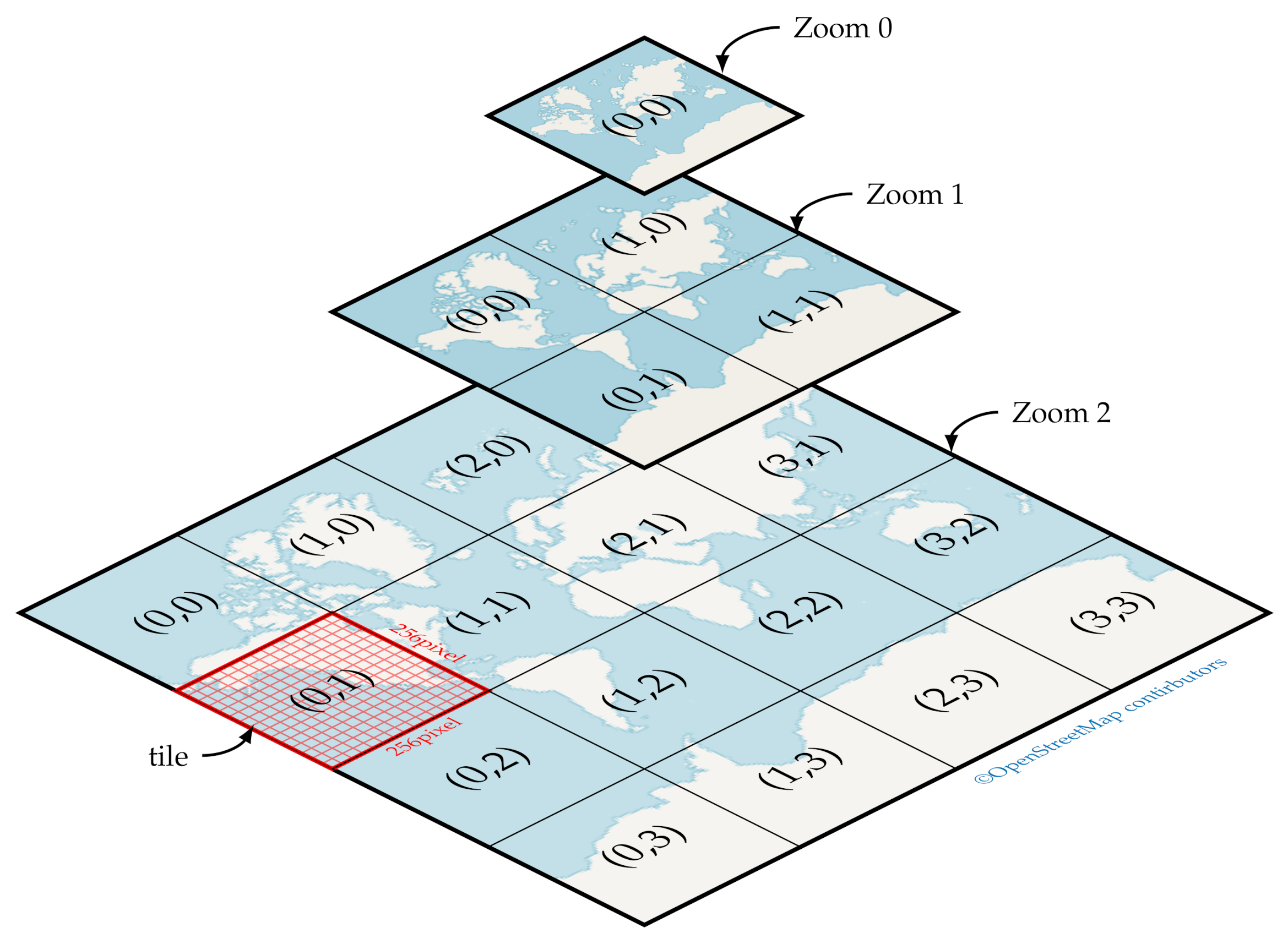
In the map tiling system using the spherical Mercator projection method, the world map is represented by a square image of 256 pixels per side (zoom level 0) by scaling the map up to 85.0511 degrees in the north–south latitude. Each time the zoom level is increased by one level, the world map of the same area is represented by a square image twice the size. A map at zoom level 1 is represented by four square images of 256 pixels per side and the images that divide this world map are called tiles. By assigning the coordinate number, , to this tile, the tile containing the specified position at the zoom level, z, can be uniquely defined as . Figure 4 shows an example of a spatial representation using the spherical Mercator projection method. The number of pixels at the zoom level, z, is , and a discretized spatial representation is generated by using these pixel coordinates.
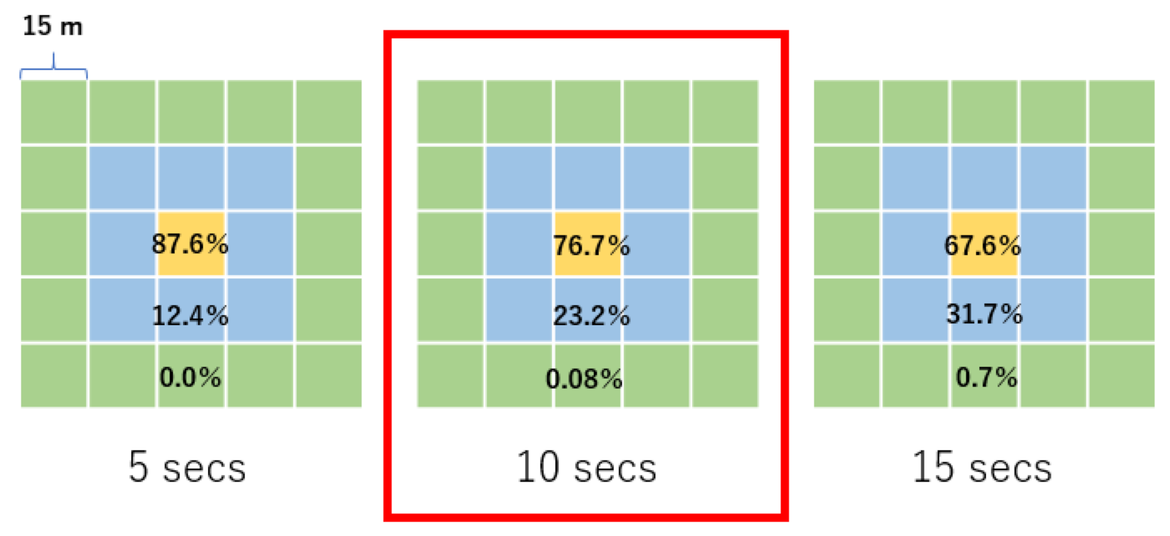
The size of the discretized grid was set to approximately 15 m considering the size of the buildings in the park and the accuracy of the data. Resampling to an appropriate sampling rate for this grid size facilitates the application of the models for sequential decision processes such as the Markovian Decision Processes (MDPs). When the sampling rate is changed to 5, 10, or 15 s, the probability of staying in the same grid, transitioning to the adjacent eight grids, and transitioning to the 16 grids, two grids ahead are calculated, respectively. Ideally, the transition probability to the neighboring grid must be maximized while minimizing the transition probability to jump two places ahead. This ensures consistency with the grid-based representation for path choice [13,22]. In particular, a sampling rate of 10 s resulted in a transition probability of approximately 23% to the neighboring grids, whereas the transition to the grid two steps ahead was suppressed to approximately 0.08 % (Figure 5). The results of resampling at this 10-second-sampling-rate were used in the following analysis.
Subsequently, the grids in which, each of the resampling data points are located, is counted and a grid network is created excluding the grids with low counts or the inaccessible grids. Consequently, the total number of target grids is obtained as 255 (Figure 6a). For the places where the transitions are not possible, such as the places which are not entrances to buildings, settings were made to prevent the transitions, even in the adjacent grids, as shown by the yellow lines in Figure 6b.
Assigning the smoothed GPS data to the grid containing the point is not sufficient. This is because it would allow for trajectories which are physically impossible and as explained earlier, the network is created to exclude physically impossible transitions. Each data point can be allocated to an appropriate grid by finding an overall plausible series to follow this defined network. The likelihood of the target grid, i, denoted by , is calculated by using the coordinate, , of the center position of the grid, i, and the position of the nth data element at time, t, is denoted by :
where A is the normalization constant and is set to half of the grid size. The time series of the grids can be obtained by solving the following problem:
Since the above equation does not change the result under logarithmic conditions, the following equation can be maximized instead:
From Equation (3), can be evaluated as follows:
Therefore, under the network constraints on the connections between the grids, the grid series which maximizes the logarithmic-likelihood can be obtained by minimizing the sum of squares in the braces of Equation (6).
The above maximization problem can be solved by using dynamic programming. The maximum value of the series, , assigned to grid, i, at time, t, can be described by using the maximum value of the series, , associated with grid, j, at time, , as follows:
where represents the correlation of the connection between the grids, i and j, and is given as:
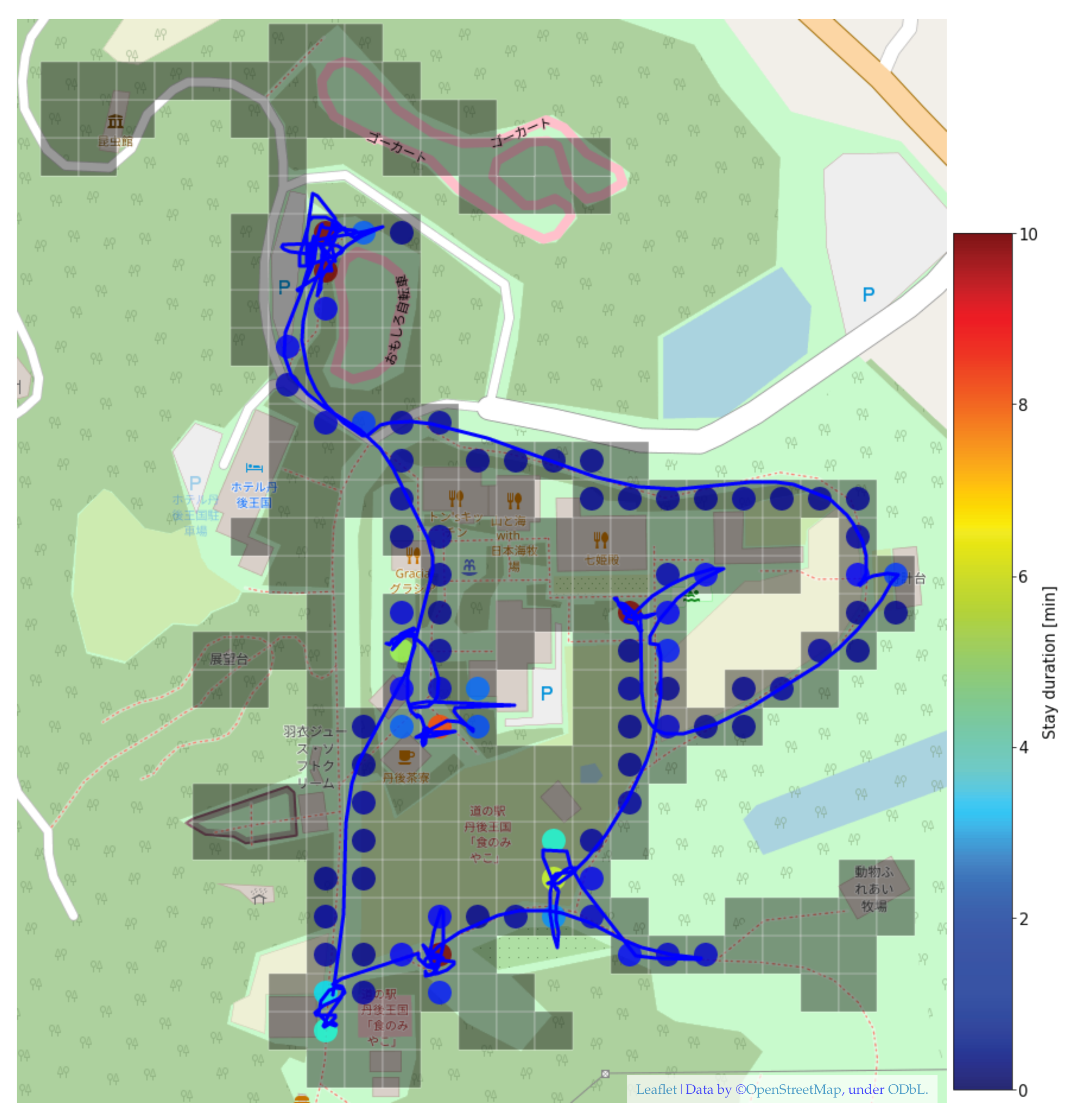
This method of spatial allocation only allows for the movement to adjacent grids for one unit of time, because it uses the correlation of the connection between the grids. Thus, even for approximately 0.08% of the data where the transitions to two grids are observed, the use of this spatial allocation method corrects for the transitions to the neighboring grids. The results of the spatial allocation are shown in Figure 7.
3.2.3. Episode Extraction
The previous section explained the process of discretization of the location information obtained from GPS data. This section describes a method to extract the stay behavior from the spatio-temporally discretized data. An episode is defined as the time from the end of the stay at one POI to the end of the stay at the next POI. Each target data element consists of multiple episodes. Each episode also includes the travel time to the destination POI. In order to extract episodes, the target POIs must be set. The 19 POIs shown in Table 1 are included in this study. The numbers in the table correspond to the numbers shown in Figure 6a.
The first step in extracting the episodes is making a decision based on the data from the discretization process of the visits to the POI locations shown in Figure 6a. Subsequently, a stay which is out of the POI position but returns immediately is considered as a continuous stay. The stays with a short residence time of 3 min or less are removed after the above process. Figure 8 shows an example of the results obtained from the above process (−1 indicates a location other than the POIs). The gray line shows the original POI stay, and the orange line indicates the processed POI stay. Additionally, the time from the end of one stay to the end of the next stay is extracted as an episode. The episodes such as episode 1, where the same POI is visited again, are combined into a single episode. A total of five episodes are extracted in this example.
3.3. Activity Scheduling Model
In this section, the dynamic activity scheduling model is described in detail to explain the extension of the model for the stated purpose. The dynamic activity scheduling model [23] is a discrete-continuous model that calculates the combined probability of an activity-choice and activity-time allocation model. The scheduling process is modeled and the activity pattern is obtained from the dynamic scheduling process.
The activity-choice model is a discrete choice model with a general multinomial logit model. Essentially, the deterministic utility component of the activity, j, is , and its choice probability is expressed as follows:
The activity time allocation model considers the allocation between the activity, j, to be performed, and the remaining set of activities, c, which are considered as composite goods. The probability of the activity time allocation is represented by the following cumulative distribution function:
where denotes a scale parameter, and and are the utilities of the activity, j, and the composite goods, c, respectively. and are given by the following equations:
where is a set of explanatory variables, and is its coefficient; and are the saturation parameters, which express the diminishing marginal utility with time. In this model, the probability of allocating time, , to activity, j, is expressed as follows:
In Habib’s (2011) activity scheduling model, the joint probability of the activity choice and the allocation time of the activity is represented by a bivariate normal distribution, given as:
where is the cumulative distribution function of the standard normal distribution, and and are transformed into the error distribution of the standard normal distribution through the inverse function of the cumulative distribution of the standard normal distribution, , as shown below:
The correlation between the activity choice and the activity time allocation is expressed through the correlation coefficient, .
In this study, the episodes are used for the activity time of each POI to estimate the activity scheduling model. It represents the time from the end of the previous activity to the end of the current activity, including the travel time to the activity location. The inclusion of the travel time to the activity location indicates that the activity time includes at least the minimum travel time between the two activity locations. Therefore, the minimum travel time between activity locations i and j, is introduced and is denoted as, , in Equations (13) and (11) as follows:
This concept is equivalent to that of the minimum required time allocation [40].
4. Results and Discussion
In this analysis, there are 262 GPS observations to be used for estimation, excluding the data where the GPS data were not captured accurately. The total number of episodes was 1042 and the average number of episodes per group was approximately four.
In the estimation, the total time spent in the facility is assumed to be presented exogenously. In this case, the final time of the data was set at the end of the stay.
The estimation is started with a model including all the potentially relevant parameters, and the parameters with low t-values were cut down in the parameter estimation results. The adjusted likelihood ratio is evaluated as a measure of the model fit, and the model with the highest value was adopted. Moreover, the initial likelihood was calculated using a model incorporating a constant value of baseline utility and with a saturation parameter [23]. Although the initial number of parameters was 478, the final number of parameters was 102. The initial and the final likelihoods were −9990.16 and −7489.72, respectively, resulting in an adjusted likelihood ratio of 0.240 (Table 4).
The subsequent sections discuss the estimation results in detail.
4.1. Activity Choice Model
The estimation results of the activity-choice model are presented in Table 2. The estimated value of “Logarithm of the time elapsed since the start of the measurement” is negative for all parameters, except for the wooden play area and the main gate, indicating that the probability of choice decreases for many POIs in the latter half of the period. The Main Gate is always the last POI. The estimate for the Main Gate is positive (0.301) for the “Logarithm of the time elapsed since the start of the measurement” and negative (−3.849) for the “Percentage of time remaining”, which together increase the probability of choice as the time spent nears the total time spent. This demonstrates that the time pressure is represented and consistent results are obtained.
The change in the utility function value is shown when the total time spent is assumed to be 3 h in Figure 9, to demonstrate the effect of the explanatory variables related to time. Although the utility value of the Main Gate is extremely small at time 0, it increases with time, and is the largest after 120 min (1/3 of the remaining time). Practically, this is not possible because of the influence of other explanatory variables, such as the location of the decision-making and the visitor’s attributes. However, it is observed that the main gate is more likely to be chosen in the latter half, which indicates that the probability of returning home increases.
Considering the group attributes, it is observed that when the gender of the representative was male, the utility of the Go-Kart Track and the Petit Petting Zoo was high. It was also observed that the utility of the food court (Seven Princess Palace) and the Main Gate increased with the increase in the age of the representatives, while the utility of the handmade experiences (Komachi Scuola) and some of the attractions including the INMOTION, the wooden play area, and the grass slide decreased. Additionally, it was observed that the larger the number of children in the group, the higher the utility of the attractions such as the Go-Kart Track, bicycle riding, the wooden play area, and grass slide, while the restaurants and cafes (Gracia, Tango Tea House, and Ton’s Kitchen) and the lookout platform were less likely to be chosen. The food court, Seven Princess Palace, also recorded a negative value; however, the value was smaller than that of the other restaurants and cafes and tended to have a smaller impact.
The distance to the location of the activity also had a significant impact on the choice. Since the utility is reduced by −0.098 per grid (approximately 15 m), the farthest distance between the POIs, i.e., the insect exhibition hall, and the petting farm (28 grids, approximately 420 m), reduces the utility by −2.744.
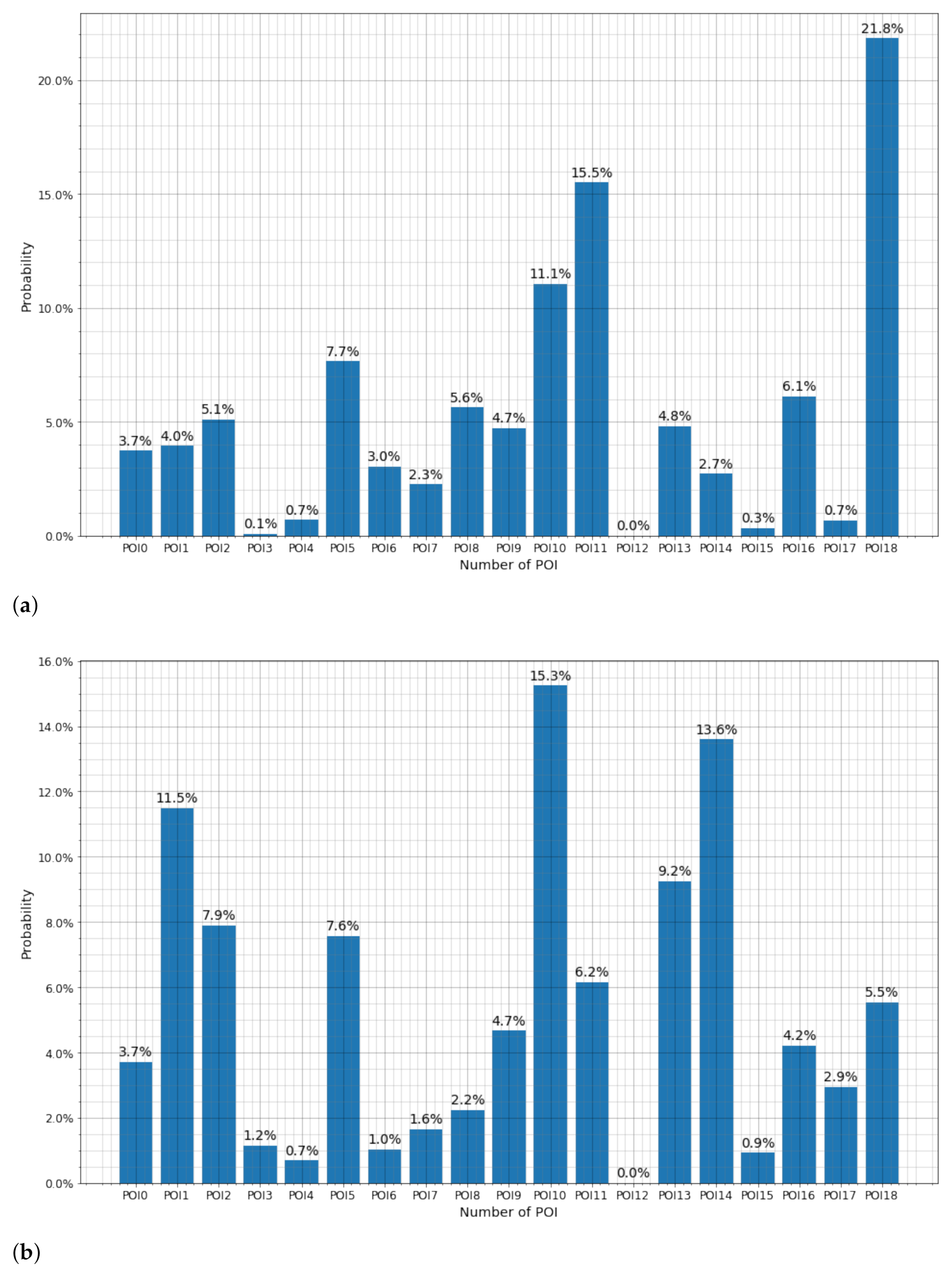
Figure 10 shows the examples of predicting the activity choice probability using the estimation results. It is assumed that the episode number is 1, the current location is the Seven Princess Palace (POI 12), the elapsed time is 60 min, and the percentage of time remaining is 2/3 (120 min). To identify the difference in the probability of choice due to the difference in the attributes of the groups, a woman in her 60 s (with no children) was assumed to be the representative in Figure 10a, and a man in their 30 s (with two children) was assumed to be the representative in Figure 10b. The predicted results showed that in the case of women in their 60 s, the most probable choices were the Main Gate, Ton’s Kitchen, and the Petting Farm. In the case of men in their 30 s, the order of choice probability was the Petit Petting Zoo, the Wooden Play Area, and the Go-Kart track, indicating that the differences in attributes significantly affect the activity choice probability. For the cases in which there are children in the group, the utility of the attractions is especially high. As mentioned above, it is observed that the probability of choosing these activities increases significantly.
4.2. Activity Time Allocation Model
The estimation of the activity time allocation model is presented in Table 3 and Table 4. The following characteristics were observed for the baseline utility shown in Table 3: In the lunch time period of 12 noon to 3 PM, positive values were recorded at the lunch places such as Ton’s Kitchen and the Seven Princess Palace, which tended to increase the length of stay. The value of the time elapsed since the start of measurement was positive for all POIs except for the Seven Princess Palace, which indicates the utility of each POI was higher in the latter half of the activity, indicating a tendency to leave more time to stay in the latter half. The parameter value for the age group of the representative was also positive in Ton’s Kitchen and the Seven Princess Palace, indicating that older people tend to spend more time in these POIs. Considering the distance to the next activity location, the estimated values were positive and consistent with the travel time during the activity time.
For the saturation parameters shown in Table 4, the smaller the value, the greater the diminution in the marginal utility, and the shorter the duration of the stay. Smaller values were obtained at the Go-Kart tracks, Nishiri, and Anju Bakery, which fitted well to the expectation, since a shorter time period is required for the Go-Kart Track per lap and since Nishiri and Anju Bakery are smaller shops with a short stay. The saturation parameters of the composite goods that contributed to the amount of time left for the rest of the activities were compared with the time of day (Figure 11); the values were relatively large in the morning and tended to decrease in the latter half of the day. This result suggested the presence of time pressure in early hours of activity scheduling. As the time pressure in activity scheduling is considered to arise from activity planning [23], more number of shorter activities are expected in the early hours because there are more planned and unexecuted activities.
5. Conclusions
In this study, we proposed a processing method for the discretization of GPS data with noise and missing data into a two-dimensional grid-based spatial representation with a high spatial resolution of 15 m. The information about the stay at the POIs was extracted from the discretized data and a dynamic activity scheduling model composed of an activity choice model and an activity time allocation model was estimated based on this information.
The estimation results of the activity choice model showed that the group attributes, such as the age of the representative and the number of children significantly affect the probability of choosing outdoor activities, such as athletic activities and grass sliding activities. Additionally, the probability of choosing the main gate increased in the latter half of the stay, confirming the effect of the time pressure. The estimated results of the activity time allocation model indicate that the time spent in restaurants and food courts tended to be longer during the lunch hour; the older the visitors, the longer they tended to stay in the restaurants and food courts. Moreover, the time variation of the saturation parameter of the composite goods suggested the existence of time pressure in the early hours. The time pressure is generated from activities planned but not yet executed.
There are no previous studies which have been able to estimate the activity choice as well as the activity time allocation from the GPS data. This study therefore contributes significantly to the literature, even if it is an analysis of the activities in a single facility. In particular, this method can formulate a novel approach for designing public spaces based on sensing data. Furthermore, the number of visitors at a newly planned space can be accurately predicted using the framework of this analysis. As such, the design of lively public spaces with the practical application of the proposed framework is a major challenge for us in the future.
In the future, collaboration and integration of the proposed framework with methods of different spatial scales can be considered. For example, in this study, the total time spent in outdoor facilities was given exogenously. However, since the total duration of stay is essentially unknown, city-scaled activity-based models can be employed to obtain the duration of stay [41,42,43]. Moreover, the proposed framework can be integrated with route choice models. The spatiotemporal discretization method in this study can be applied to recursive-type route choice models, such as the recursive logit model [44]. Such applications facilitate the integrated modeling of the complex decision-making behavior of pedestrians.
Author Contributions
Conceptualization, K.H. and T.Y.; methodology, K.H.; software, K.H.; validation, K.H.; formal analysis, K.H.; investigation, K.H.; resources, K.H. and T.Y.; data curation, K.H. Writing—original draft preparation, K.H.; writing—review and editing, K.H. and T.Y.; visualization, K.H.; supervision, T.Y.; project administration, K.H. and T.Y.; funding acquisition, K.H. and T.Y. All authors have read and agreed to the published version of the manuscript.
Funding
This research received no external funding.
Institutional Review Board Statement
Not applicable.
Informed Consent Statement
Informed consent was obtained from all subjects involved in the study.
Data Availability Statement
Not applicable.
Conflicts of Interest
The authors declare that there is no conflict of interest.
Abbreviations
The following abbreviations are used in this manuscript:
| BLE | Bluetooth Low Energy |
| GPS | Global Positioning System |
| POIs | Point of Interests |
References
- Carmona, M. Place value: Place quality and its impact on health, social, economic and environmental outcomes. J. Urban Des. 2019, 24, 1–48. [Google Scholar] [CrossRef] [Green Version]
- Mehta, V. Lively streets: Determining environmental characteristics to support social behavior. J. Plan. Educ. Res. 2007, 27, 165–187. [Google Scholar] [CrossRef]
- Anderson, J.; Ruggeri, K.; Steemers, K.; Huppert, F. Lively social space, well-being activity, and urban design: Findings from a low-cost community-led public space intervention. Environ. Behav. 2017, 49, 685–716. [Google Scholar] [CrossRef]
- Hoogendoorn, S.P.; Bovy, P.H. Pedestrian route-choice and activity scheduling theory and models. Transp. Res. Part B Methodol. 2004, 38, 169–190. [Google Scholar] [CrossRef]
- Antonini, G.; Bierlaire, M.; Weber, M. Discrete choice models of pedestrian walking behavior. Transp. Res. Part Methodol. 2006, 40, 667–687. [Google Scholar] [CrossRef]
- Blue, V.J.; Adler, J.L. Cellular automata microsimulation for modeling bi-directional pedestrian walkways. Transp. Res. Part Methodol. 2001, 35, 293–312. [Google Scholar] [CrossRef]
- Helbing, D.; Farkas, I.; Vicsek, T. Simulating dynamical features of escape panic. Nature 2000, 407, 487. [Google Scholar] [CrossRef] [Green Version]
- Moussaïd, M.; Perozo, N.; Garnier, S.; Helbing, D.; Theraulaz, G. The walking behaviour of pedestrian social groups and its impact on crowd dynamics. PLoS ONE 2010, 5, e10047. [Google Scholar] [CrossRef] [Green Version]
- Treuille, A.; Cooper, S.; Popović, Z. Continuum crowds. ACM Trans. Graph. (TOG) 2006, 25, 1160–1168. [Google Scholar] [CrossRef]
- Duives, D.C.; Mahmassani, H.S. Exit choice decisions during pedestrian evacuations of buildings. Transp. Res. Rec. 2012, 2316, 84–94. [Google Scholar] [CrossRef]
- Haghani, M.; Sarvi, M. Pedestrian crowd tactical-level decision making during emergency evacuations. J. Adv. Transp. 2016, 50, 1870–1895. [Google Scholar] [CrossRef]
- Lo, S.M.; Huang, H.C.; Wang, P.; Yuen, K. A game theory based exit selection model for evacuation. Fire Saf. J. 2006, 41, 364–369. [Google Scholar] [CrossRef]
- Asano, M.; Iryo, T.; Kuwahara, M. Microscopic pedestrian simulation model combined with a tactical model for route choice behaviour. Transp. Res. Part Emerg. Technol. 2010, 18, 842–855. [Google Scholar] [CrossRef]
- Nasir, M.; Lim, C.P.; Nahavandi, S.; Creighton, D. Prediction of pedestrians routes within a built environment in normal conditions. Expert Syst. Appl. 2014, 41, 4975–4988. [Google Scholar] [CrossRef]
- Wang, Z.; Oyama, Y.; Scarinci, R.; Bierlaire, M.; Geroliminis, N. Pedestrian activity schedule models: Review and promises. In Proceedings of the 18th Swiss Transport Research Conference (STRC), Monte Verita/Ascona, Switzerland, 16–18 May 2018. [Google Scholar]
- Liu, X.; Usher, J.M.; Strawderman, L. An analysis of activity scheduling behavior of airport travelers. Comput. Ind. Eng. 2014, 74, 208–218. [Google Scholar] [CrossRef]
- Danalet, A.; Tinguely, L.; de Lapparent, M.; Bierlaire, M. Location choice with longitudinal WiFi data. J. Choice Model. 2016, 18, 1–17. [Google Scholar] [CrossRef] [Green Version]
- Beaulieu, A.; Farooq, B. A dynamic mixed logit model with agent effect for pedestrian next location choice using ubiquitous Wi-Fi network data. Int. J. Transp. Sci. Technol. 2019, 8, 280–289. [Google Scholar] [CrossRef]
- Danalet, A.; Farooq, B.; Bierlaire, M. A Bayesian approach to detect pedestrian destination-sequences from WiFi signatures. Transp. Res. Part C Emerg. Technol. 2014, 44, 146–170. [Google Scholar] [CrossRef] [Green Version]
- Borst, H.C.; Miedema, H.M.; de Vries, S.I.; Graham, J.M.; van Dongen, J.E. Relationships between street characteristics and perceived attractiveness for walking reported by elderly people. J. Environ. Psychol. 2008, 28, 353–361. [Google Scholar] [CrossRef]
- Borgers, A.; Timmermans, H. A model of pedestrian route choice and demand for retail facilities within inner-city shopping areas. Geogr. Anal. 1986, 18, 115–128. [Google Scholar] [CrossRef] [Green Version]
- Hidaka, K.; Hayakawa, K.; Nishi, T.; Usui, T.; Yamamoto, T. Generating pedestrian walking behavior considering detour and pause in the path under space-time constraints. Transp. Res. Part Emerg. Technol. 2019, 108, 115–129. [Google Scholar] [CrossRef]
- Habib, K.M.N. A random utility maximization (RUM) based dynamic activity scheduling model: Application in weekend activity scheduling. Transportation 2011, 38, 123–151. [Google Scholar] [CrossRef]
- Fan, Z.; Song, X.; Shibasaki, R. Cityspectrum: A non-negative tensor factorization approach. In Proceedings of the 2014 ACM International Joint Conference on Pervasive and Ubiquitous Computing, Washington, DC, USA, 13–17 September 2014; pp. 213–223. [Google Scholar]
- Furletti, B.; Cintia, P.; Renso, C.; Spinsanti, L. Inferring human activities from GPS tracks. In Proceedings of the 2nd ACM SIGKDD International Workshop on Urban Computing, Chicago, IL, USA, 11–14 August 2013; pp. 1–8. [Google Scholar]
- Coni, M.; Maltinti, F.; Pinna, F.; Rassu, N.; Garau, C.; Barabino, B.; Maternini, G. On-Board Comfort of Different Age Passengers and Bus-Lane Characteristics. In International Conference on Computational Science and Its Applications; Springer: Berlin/Heidelberg, Germany, 2020; pp. 658–672. [Google Scholar]
- Kasemsuppakorn, P.; Karimi, H.A. A pedestrian network construction algorithm based on multiple GPS traces. Transp. Res. Part C Emerg. Technol. 2013, 26, 285–300. [Google Scholar] [CrossRef]
- Oyama, Y.; Hato, E. Link-based measurement model to estimate route choice parameters in urban pedestrian networks. Transp. Res. Part Emerg. Technol. 2018, 93, 62–78. [Google Scholar] [CrossRef]
- Han, T.; Zhao, J.; Li, W. Smart-Guided Pedestrian Emergency Evacuation in Slender-Shape Infrastructure with Digital Twin Simulations. Sustainability 2020, 12, 9701. [Google Scholar] [CrossRef]
- Yamamoto, K.; Kokubo, S.; Nishinari, K. Simulation for pedestrian dynamics by real-coded cellular automata (RCA). Phys. A Stat. Mech. Its Appl. 2007, 379, 654–660. [Google Scholar] [CrossRef]
- Xu, W.; Liu, L.; Zlatanova, S.; Penard, W.; Xiong, Q. A pedestrian tracking algorithm using grid-based indoor model. Autom. Constr. 2018, 92, 173–187. [Google Scholar] [CrossRef]
- Ziebart, B.D.; Ratliff, N.; Gallagher, G.; Mertz, C.; Peterson, K.; Bagnell, J.A.; Hebert, M.; Dey, A.K.; Srinivasa, S. Planning-based prediction for pedestrians. In Proceedings of the IEEE/RSJ International Conference on Intelligent Robots and Systems 2009—IROS 2009, St. Louis, MI, USA, 11–15 October 2009; pp. 3931–3936. [Google Scholar]
- Sarjala, S. Built environment determinants of pedestrians’ and bicyclists’ route choices on commute trips: Applying a new grid-based method for measuring the built environment along the route. J. Transp. Geogr. 2019, 78, 56–69. [Google Scholar] [CrossRef]
- Zhang, J. A model of time use and expenditure of pedestrians in city centers. In Pedestrian Behavior; Emerald Group Publishing Limited: Bingley, UK, 2009. [Google Scholar]
- Fukuyama, S.; Hato, E. Pedestrian velocityand direction choice problem based on probabilistic activity domain. J. City Plan. Inst. Jpn. 2016, 51, 688–694. (In Japanese) [Google Scholar]
- Yamamoto, T.; Usui, T.; Nakamura, N.; Morikawa, T. Activity-travel behavior survey at tourist attraction by BLE in comparison with GPS. In Proceedings of the Launch Workshop of NECTOR Cluster 5, Tourism and Transport: Exploration of Interdependecies, Lugano, Switzerland, 29 September–1 October 2016. [Google Scholar]
- Rauch, H.E.; Tung, F.; Striebel, C.T. Maximum likelihood estimates of linear dynamic systems. AIAA J. 1965, 3, 1445–1450. [Google Scholar] [CrossRef]
- Krajewski, R.; Bock, J.; Kloeker, L.; Eckstein, L. The highd dataset: A drone dataset of naturalistic vehicle trajectories on german highways for validation of highly automated driving systems. In Proceedings of the 2018 21st International Conference on Intelligent Transportation Systems (ITSC), Maui, HI, USA, 4–7 November 2018; pp. 2118–2125. [Google Scholar]
- Wilson, A.M.; Hubel, T.Y.; Wilshin, S.D.; Lowe, J.C.; Lorenc, M.; Dewhirst, O.P.; Bartlam-Brooks, H.L.; Diack, R.; Bennitt, E.; Golabek, K.A.; et al. Biomechanics of predator–prey arms race in lion, zebra, cheetah and impala. Nature 2018, 554, 183–188. [Google Scholar] [CrossRef]
- Van Nostrand, C.; Sivaraman, V.; Pinjari, A.R. Analysis of long-distance vacation travel demand in the United States: A multiple discrete–continuous choice framework. Transportation 2013, 40, 151–171. [Google Scholar] [CrossRef]
- Roorda, M.J.; Miller, E.J.; Habib, K.M. Validation of TASHA: A 24-h activity scheduling microsimulation model. Transp. Res. Part A Policy Pract. 2008, 42, 360–375. [Google Scholar] [CrossRef] [Green Version]
- Goulias, K.G.; Bhat, C.R.; Pendyala, R.M.; Chen, Y.; Paleti, R.; Konduri, K.C.; Huang, G.; Hu, H.H. Simulator of activities, greenhouse emissions, networks, and travel (SimAGENT) in Southern California: Design, implementation, preliminary findings, and integration plans. In Proceedings of the 2011 IEEE Forum on Integrated and Sustainable Transportation Systems, Vienna, Austria, 29 June–1 July 2011; pp. 164–169. [Google Scholar]
- Hidaka, K.; Ohno, H.; Shiga, T. Understanding Human Mobility and Activity in Multiple Non-identifiable Statistics. In Proceedings of the 14th International Conference on Computers in Urban Planning and Urban Management, Cambridge, MA, USA, 7–10 July 2015. [Google Scholar]
- Fosgerau, M.; Frejinger, E.; Karlstrom, A. A link based network route choice model with unrestricted choice set. Transp. Res. Part B Methodol. 2013, 56, 70–80. [Google Scholar] [CrossRef] [Green Version]
Figure 1.
Schematic diagram of the smoothing process. (a) GPS data before processing; (b) Data after the smoothing process.
Figure 1.
Schematic diagram of the smoothing process. (a) GPS data before processing; (b) Data after the smoothing process.

Figure 2.
Smoothing process procedure.

Figure 3.
Application example of smoothing process (yellow: BLE receiver, blue: GPS data before processing, red: data after smoothing process).
Figure 3.
Application example of smoothing process (yellow: BLE receiver, blue: GPS data before processing, red: data after smoothing process).

Figure 4.
Spatial representation by spherical Mercator projection method.

Figure 5.
Relationship between sampling rate and transition probability.

Figure 6.
(a) Networks where the numbers in the figure correspond to the POI numbers; (b) Setting up a grid that cannot be transitioned.
Figure 6.
(a) Networks where the numbers in the figure correspond to the POI numbers; (b) Setting up a grid that cannot be transitioned.

Figure 7.
The results of the spatial allocation. The allocation results are represented by circles, and the color of the circle represents the stay duration.
Figure 7.
The results of the spatial allocation. The allocation results are represented by circles, and the color of the circle represents the stay duration.

Figure 8.
An example of extracted episodes.

Figure 9.
An example of time variation of utility function.

Figure 10.
Examples of predicting the activity choice probability (current position: Seven Princess Palace, number of episode: 1, time elapsed: 60 min; percentage of remaining time: 2/3). (a) Representatives: 60–69 years women with no children; (b) Representatives: 30–39 years men with 2 children.
Figure 10.
Examples of predicting the activity choice probability (current position: Seven Princess Palace, number of episode: 1, time elapsed: 60 min; percentage of remaining time: 2/3). (a) Representatives: 60–69 years women with no children; (b) Representatives: 30–39 years men with 2 children.

Figure 11.
Saturation parameter values for composite goods by time.


Table 1.
Target POIs.
| No. | Name | Types | Description |
|---|---|---|---|
| 0 | Insect Exhibition Hall | Activities | Exhibits of beetles and stag beetles from around the world |
| 1 | Go-Karts Track | Attractions | Go-kart experience for kids and adults |
| 2 | Bicycle Riding | Attractions | Unique bicycle riding experience |
| 3 | Komachi Scuola | Activities | Bread and ice cream making experience |
| 4 | Nishiri (Pickles Shop) | Shopping | Japanese pickled vegetable shop |
| 5 | Anju Bakery | Shopping | Freshly baked bread shop |
| 6 | Gracia | Foods | Restaurant |
| 7 | Tango Tea House | Foods | Japanese sweets and tea cafe |
| 8 | Lookout Platform | Activities | |
| 9 | Hagoromo Juice and Soft Ice Cream | Foods | Soft serve ice cream and fresh juice bar |
| 10 | Petit Petting Zoo | Activities | Petting zoo for sheeps, goats, rabbits, and tortoises |
| 11 | Ton’s Kitchen | Foods | Restaurant |
| 12 | Seven Princess Palace | Foods | Family-friendly food court |
| 13 | INMOTION | Attractions | Experience the next generation of standing electric motorcycles |
| 14 | Wooden Play Area | Attractions | Athletic field for kids |
| 15 | Clock Tower | Activities | |
| 16 | Petting Farm | Activities | Interacting with sheep and ponies, riding ponies |
| 17 | Grass Slide | Attractions | 48 m long grass slide |
| 18 | Main Gate | Shopping | The main gate with souvenirs shop and farmer’s market |
Table 2.
Estimated results (activity choice model).
| Variables | Name of POI | Type of POI | POI Number | Parameters | t-Values |
|---|---|---|---|---|---|
| Alternative Specific Constant (ASC) | |||||
| Lookout Platform | Activities | 8 | −0.576 | −1.97 | |
| Number of Episode | |||||
| Go-Kart Track | Attractions | 1 | −0.144 | −1.63 | |
| Gracia | Foods | 6 | 0.350 | 2.29 | |
| Hagoromo Juice and Soft Ice Cream | Foods | 9 | −0.236 | −1.94 | |
| Ton’s Kitchen | Foods | 11 | −0.153 | −1.77 | |
| Wooden Play Area | Attractions | 14 | −0.113 | −1.09 | |
| Grass Slide | Attractions | 17 | 0.176 | 1.56 | |
| 12 noon to 3 PM | |||||
| Seven Princess Palace | Foods | 12 | 0.346 | 1.67 | |
| Petting Farm | Activities | 16 | 0.576 | 2.81 | |
| After 3 PM | |||||
| Anju Bakery | Shopping | 5 | −0.691 | −1.52 | |
| Ton’s Kitchen | Foods | 11 | −1.161 | −1.77 | |
| Logarithm of the time elapsed since the measurement started (10 s unit time) | |||||
| Bicycle Riding | Attractions | 2 | −0.137 | −2.99 | |
| Nishiri | Shopping | 4 | −0.518 | −7.57 | |
| Anju Bakery | Shopping | 5 | −0.150 | −3.89 | |
| Gracia | Foods | 6 | −0.329 | −3.45 | |
| Tango Tea House | Foods | 7 | −0.177 | −2.14 | |
| Hagoromo Juice and Soft Ice Cream | Foods | 9 | −0.121 | −2.48 | |
| Seven Princess Palace | Foods | 12 | −0.102 | −2.47 | |
| Wooden Play Area | Attractions | 14 | 0.101 | 1.31 | |
| Clock Tower | Activities | 15 | −0.193 | −1.37 | |
| Grass Slide | Attractions | 17 | −0.188 | −2.42 | |
| Main Gate | Shopping | 18 | 0.301 | 5.33 | |
| Representative’s gender (Men = 1, Women = 0) | |||||
| Go-Kart Track | Attractions | 1 | 0.549 | 2.26 | |
| Petit Petting Zoo | Activities | 10 | 0.331 | 2.00 | |
| Representative’s age (in 10 years) | |||||
| Komachi Scuola | Activities | 3 | −0.848 | −6.34 | |
| Tango Tea House | Foods | 7 | −0.108 | −1.37 | |
| Seven Princess Palace | Foods | 12 | 0.231 | 4.12 | |
| INMOTION | Attractions | 13 | −0.220 | −4.55 | |
| Wooden Play Area | Attractions | 14 | −0.346 | −3.55 | |
| Clock Tower | Activities | 15 | −0.344 | −1.16 | |
| Grass Slide | Attractions | 17 | −0.243 | −2.93 | |
| Main Gate | Shopping | 18 | 0.330 | 3.78 | |
| Number of children in the group | |||||
| Go-Karts Track | Attractions | 1 | 0.264 | 2.60 | |
| Bicycle Riding | Attractions | 2 | 0.223 | 1.56 | |
| Gracia | Foods | 6 | −0.537 | −2.20 | |
| Tango Tea House | Foods | 7 | −0.315 | −1.21 | |
| Lookout Platform | Activities | 8 | −0.455 | −1.92 | |
| Ton’s Kitchen | Foods | 11 | −0.457 | −2.81 | |
| Seven Princess Palace | Foods | 12 | −0.121 | −1.44 | |
| Wooden Play Area | Attractions | 14 | 0.289 | 2.73 | |
| Petting Farm | Activities | 16 | −0.182 | −1.54 | |
| Grass Slide | Attractions | 17 | 0.370 | 2.77 | |
| Main Gate | Shopping | 18 | −0.187 | −1.59 | |
| Already visited | |||||
| Petit Petting Zoo | Activities | 10 | −0.891 | −2.53 | |
| Distance from the previous activity location (minimum number of steps) | |||||
| Common | − | − | −0.098 | −11.68 | |
| Percentage of remaining time (remaining time/total time spent) | |||||
| Bicycle Riding | Attraction | 2 | 0.636 | 1.80 | |
| Anju Bakery | Shopping | 5 | 0.329 | 1.60 | |
| Main Gate | Shopping | 18 | −3.849 | −8.48 | |
| Residents of Kyoto Prefecture | |||||
| Bicycle Riding | Attractions | 2 | −0.645 | −1.95 | |
| Gracia | Foods | 6 | −1.125 | −1.93 | |
Table 3.
Estimated results (activity time allocation model).
| Variables | Name of POI | Type of POI | POI Number | Parameters | t-Values |
|---|---|---|---|---|---|
| Number of episode | |||||
| Insect Exhibition Hall | Activities | 0 | 0.313 | 1.28 | |
| INMOTION | Attractions | 13 | 0.352 | 2.74 | |
| Clock Tower | Activities | 15 | 0.778 | 1.59 | |
| Petting Farm | Activities | 16 | 0.212 | 1.50 | |
| 12 noon to 3 PM | |||||
| Ton’s Kitchen | Foods | 11 | 0.859 | 1.83 | |
| Seven Princess Palace | Foods | 12 | 1.105 | 2.34 | |
| Logarithm of the time elapsed since the measurement started (10 s unit time) | |||||
| Go-Karts Track | Attractions | 1 | 0.418 | 3.81 | |
| Bicycle Riding | Attractions | 2 | 0.272 | 2.44 | |
| Anju Bakery | Shopping | 5 | 0.232 | 2.31 | |
| Petit Petting Zoo | Activities | 10 | 0.283 | 3.86 | |
| Ton’s Kitchen | Foods | 11 | 0.224 | 1.16 | |
| Seven Princess Palace | Foods | 12 | −0.244 | −3.51 | |
| Wooden Play Area | Attractions | 14 | 0.312 | 3.24 | |
| Petting Farm | Activities | 16 | 0.173 | 1.57 | |
| Grass Slide | Attractions | 17 | 0.221 | 2.06 | |
| Main Gate | Shopping | 18 | 0.399 | 3.74 | |
| Representative’s age groups (ten−year age groups) | |||||
| Ton’s Kitchen | Foods | 11 | 0.662 | 2.81 | |
| Seven Princess Palace | Foods | 12 | 0.141 | 1.22 | |
| Number of children in the group | |||||
| Petit Petting Zoo | Activities | 10 | −0.463 | −2.12 | |
| Main Gate | Shopping | 18 | −0.156 | −1.59 | |
| Distance from the previous activity location (minimum number of steps) | |||||
| Common | − | − | 0.053 | 5.15 | |
Table 4.
Estimated results (Saturation parameters et al.).
| Variables | Name of POI | Type of POI | POI Number | Parameters | Standard Errors |
|---|---|---|---|---|---|
| Saturation parameters (POI) | |||||
| Insect Exhibition Hall | Activities | 0 | −0.984 | 0.116 | |
| Go-Karts Track | Attractions | 1 | −1.371 | 0.140 | |
| Bicycle Riding | Attractions | 2 | −0.840 | 0.121 | |
| Komachi Scuola | Activities | 3 | −0.773 | 0.083 | |
| Nishiri | Shopping | 4 | −1.075 | 0.148 | |
| Anju Bakery | Shopping | 5 | −1.041 | 0.122 | |
| Gracia | Foods | 6 | −0.667 | 0.127 | |
| Tango Tea House | Foods | 7 | −0.815 | 0.082 | |
| Lookout Platform | Activities | 8 | −0.842 | 0.115 | |
| Hagoromo Juice and Soft Ice Cream | Foods | 9 | −0.845 | 0.057 | |
| Petit Petting Zoo | Activities | 10 | −0.861 | 0.108 | |
| Ton’s Kitchen | Foods | 11 | −0.919 | 0.216 | |
| Seven Princess Palace | Foods | 12 | −0.367 | 0.087 | |
| INMOTION | Attractions | 13 | −0.993 | 0.086 | |
| Wooden Play Area | Attractions | 14 | −1.070 | 0.119 | |
| Clock Tower | Activities | 15 | −0.984 | 0.366 | |
| Petting Farm | Activities | 16 | −0.920 | 0.092 | |
| Grass Slide | Attractions | 17 | −0.616 | 0.100 | |
| Main Gate | Shopping | 18 | 0.195 | 0.169 | |
| Saturation parameters (composite goods) | |||||
| 9 AM to 9:59 AM | − | − | −0.094 | 0.073 | |
| 10 AM to 10:59 AM | − | − | 0.010 | 0.060 | |
| 11 AM to 11:59 AM | − | − | −0.120 | 0.045 | |
| 12 noon to 12:59 noon | − | − | −0.054 | 0.048 | |
| 1 PM to 1:59 PM | − | − | −0.109 | 0.055 | |
| 2 PM to 2:59 PM | − | − | −0.143 | 0.049 | |
| 3 PM to 3:59 PM | − | − | −0.295 | 0.069 | |
| 4 PM to 4:59 PM | − | − | −0.217 | 0.100 | |
| 5 PM to 5:59 PM | − | − | −0.308 | 0.412 | |
| 6 PM to 6:59 PM | − | − | −0.188 | 0.311 | |
| Scale parameter | 1.060 | 0.040 | |||
| Correlation coefficient | −0.350 | 0.062 | |||
| Log likelihood of constant−only model | −9990.16 | ||||
| Log likelihood of full model | −7489.72 | ||||
| Adjusted Rho−square value | 0.240 | ||||
Publisher’s Note: MDPI stays neutral with regard to jurisdictional claims in published maps and institutional affiliations. |
© 2021 by the authors. Licensee MDPI, Basel, Switzerland. This article is an open access article distributed under the terms and conditions of the Creative Commons Attribution (CC BY) license (https://creativecommons.org/licenses/by/4.0/).
Share and Cite
MDPI and ACS Style
Hidaka, K.; Yamamoto, T. Activity Scheduling Behavior of the Visitors to an Outdoor Recreational Facility Using GPS Data. Sustainability 2021, 13, 4871. https://0-doi-org.brum.beds.ac.uk/10.3390/su13094871
AMA Style
Hidaka K, Yamamoto T. Activity Scheduling Behavior of the Visitors to an Outdoor Recreational Facility Using GPS Data. Sustainability. 2021; 13(9):4871. https://0-doi-org.brum.beds.ac.uk/10.3390/su13094871
Chicago/Turabian StyleHidaka, Ken, and Toshiyuki Yamamoto. 2021. "Activity Scheduling Behavior of the Visitors to an Outdoor Recreational Facility Using GPS Data" Sustainability 13, no. 9: 4871. https://0-doi-org.brum.beds.ac.uk/10.3390/su13094871
Note that from the first issue of 2016, this journal uses article numbers instead of page numbers. See further details here.