
Modeling Urban Road Scenarios to Evaluate Intersection Visibility


1
Departamento de Ingeniería del Transporte, Territorio y Urbanismo, Universidad Politécnica de Madrid, 28040 Madrid, Spain
2
Department of Chemical and Biological Engineering, Iowa State University, Ames, IA 50011, USA
3
Department of Statistics, Iowa State University, Ames, IA 50011, USA
*
Author to whom correspondence should be addressed.
Sustainability 2022, 14(1), 354; https://0-doi-org.brum.beds.ac.uk/10.3390/su14010354
Submission received: 5 October 2021
/
Revised: 21 December 2021
/
Accepted: 27 December 2021
/
Published: 29 December 2021
(This article belongs to the Special Issue Highway Models and Sustainability)
Abstract
:Road safety is key to sustainable mobility. Rapid technological advances have allowed several road safety-related analyses, previously performed in situ, to be conducted virtually. These virtual analyses benefit understanding of how roads operate and how users perceive them. Additionally, they facilitate the assessment of several parameters that are fundamental to road design and operation. The available sight distance (ASD) is one of these parameters that, if not provided adequately, could alter the proper functioning of roads. This study presents a framework to assess the impact of certain features on visibility. First, the ASD is estimated using a geographic information system (GIS)-based procedure with LiDAR-derived three-dimensional (3D) models. Afterward, obstructions are detected and categorized. If the obstruction cannot be removed, their redesign or relocation is simulated to re-run the analysis. These simulations are performed using 3D city objects, and their results are statistically evaluated, providing evidence as to their effects on visibility. The results proved that the procedure helped achieve the efficient use of roadside space, while including safety concerns. Additionally, this study reflects the need for more inspections on the impact of on-street parking on drivers’ fields of view.
1. Introduction
Road safety has constituted one of the significant challenges of recent times. It is a critical component of achieving sustainable mobility [1]. Among the different efforts to improve road safety, geometric design aims to provide efficient and convenient infrastructure to support safe driving, riding, cycling and walking.
Road and highway design guidelines state the crucial role of the visual sensing of information in driving tasks [2]. The visual search activity and operations of drivers vary according to the road geometry and surroundings [3]. These variations are included in the calculations that determine the dimensions and disposition of geometric design elements. Visibility is mainly provided through adequate sight distances. Sight distance is the length of roadway visible to drivers [4]. It is usually provisioned in new designs but could be altered if changes in the cross-section of the road or the roadside take place. Changes in the cross-section could be caused by installing safety elements, modifications of the dimensions and alignments of the roadway, bicycle infrastructure or sidewalks, changes in shoulder use, and many other causes. Roadside changes could be the product of vegetation growth, new developments, new elements of street fixtures and furnishings, etc. Because of these changes, sight distances should be estimated periodically on existing roads.
Urban contexts put more pressure on the constraints that rule the geometric design of roads due to their usually high-density development, minor setbacks, mixed land uses, etc. [4,5]. Moreover, designers are expected to make the most effective use of the shared space between motorized and non-motorized users (and their distinct operating speeds, capabilities, reaction times, etc.), along with a wide variety of city needs. The quality of urban circulation is governed by the appropriate functioning of its intersections [6].
Correct intersection operation requires the adequate provisioning of sight distances. Research has shown that drivers’ operating characteristics and visual search behavior vary depending on their experience, the type of intersection (T-type, X-type, etc.), the maneuver involved, and the complexity of the surroundings [7,8].
In addition to having a clear view of the intersection, drivers should spot pedestrians and other vulnerable road users that intend to cross the roadway. Vulnerable road users also require enough visibility to notice motorists and safely interact or negotiate with them. Because of all that, the proper functioning of road intersections depends significantly on the provisioning of sight distances.
Active transportation modes are being actively encouraged worldwide due to their multiple benefits. Consequently, it is crucial to ensure that current roads can safely accommodate this wide array of users. In addition, emerging micromobility services, commonly used for last- and first-mile trips, nowadays contribute to the increasing number of vulnerable road users sharing the road [9]. These vulnerable road users also require the evaluation of their existing sight distances. Nonetheless, recent studies assessing sight distances on existing facilities focus on the roadway, considering the driver as the central observer [10,11,12].
In addition to the complexities added by their multiple users, urban settings tend to encompass a more diverse range of road obstructions in both their cross-sections and roadsides than rural settings. Moreover, despite having a lower percentage of road accidents (38% of all accidents in the European Union in 2017 [13]), most fatalities involving vulnerable road users occur in urban environments [14].
As sight distances play a crucial role in road safety, this paper proposes a methodology to estimate them. The focus is on urban intersections as these are the road sections with a higher presence of conflicts involving vulnerable road users [13]. This research aims to help the process that follows the identification of a sight obstruction. Once the visual obstacle is detected, solutions are proposed by modifying the existing road setting. These solutions could involve removing, relocating, or replacing obstructing elements, creating different scenarios. After that modification is completed, the visibility evaluation is carried out in each created scenario. The results of the real scenario are then compared to the modified ones. The main goal of this paper is to present a framework that assesses obstructions and assists decision-making. Its focus is on handling obstructions rather than solely focusing on their detection. It is intended to serve as a tool for design and planning based on off-site evaluations.
This paper is organized as follows: the next section presents the main findings of the literature review. The following section details the novel procedure and presents practical experiments based on common road obstructions. A description of the case study follows this. Lastly, the results are discussed, followed by the main conclusions.
2. Literature Review
Adequate sight distances tend to be appropriately provisioned in new designs. Sufficient visibility is ensured, considering sight distances as fundamental parameters in alignment and profile elements. When it comes to existing roads, as design conditions change, guidelines specify procedures to estimate available sight distances and compare them to required ones [4,15,16]. These estimations could be performed in situ, employing field measurements. However, site works alter traffic and endanger the staff [17]. Because of this, present studies propose off-site methodologies that model the road using geospatial data. Thanks to advances in software, data acquisition, and computer power, these evaluations can be performed virtually using three-dimensional (3D) road models [11,18,19]. These virtual models of the road not only assist geometric design applications but also aid in road inventories [20], automated and assisted driving [21], and other transportation applications [22].
The majority of the revised contributions have been developed to evaluate the available sight distance (ASD) required to perform stopping maneuvers to be compared with the stopping sight distance (SSD). SSD is the distance that drivers need to safely stop their vehicle when an unexpected object appears in their way.
In 2005, Khattak and Shamayleh presented a procedure to determine highways’ stopping and passing sight distances. They employed light detection and ranging (LiDAR) data and geographic information system (GIS) software. Among the literature revised herein, these authors were the first to use LiDAR to estimate sight distances. This study employed digital terrain models (DTMs) to model the road and environment and used the functionalities of the software ArcGIS to determine the available sight distance [23]. In 2010, Zarinš proposed a methodology to calculate the sight distances required for stopping using digital terrain models (to model the road and adjacent environments) and GPS data (to model the drivers’ trajectories). The sight distances were obtained using an algorithm that evaluated the unobstructed sightlines connecting the observers and targets [24]. Subsequently, more studies evaluated the available sight distances with global navigation satellite systems (GNSS) data [25].
Other contributions have focused on evaluating the ASD needed to drive safely at road intersections and comparing them with the required intersection sight distance (ISD) [26,27,28]. ISD is the distance required by a road user approaching the intersection (or stopping at its entry) to view it and drive through it adequately [5,12]. As these evaluations require updated data to depict the road settings, most contributions on the subject have employed LiDAR systems to acquire the 3D data used to model the roadway and roadside. Airborne, terrestrial, and car-mounted systems (commonly referred to as mobile LiDAR systems (MLSs)) have been put into use. Khattak et al. [26] evaluated equally spaced sightlines within the required sight triangle; Tsai et al. [27] compared the viewshed area obtained from an observer and compared it to its necessary sight triangle. These two publications used digital surface models (DSMs) to recreate the road and surroundings. Olsen et al. [28] also used viewsheds from observers. They modeled the road environment utilizing voxels created from LiDAR point clouds. These voxels were also used to assess ISD in Jung et al. [17]. These contributions were intended to detect and quantify the effect of visual obstructions on driver visibility.
Recent studies have presented evaluations performed directly on the cloud of LiDAR points. They estimate sight distances directly on a filtered and clean cloud of points or voxels. This current trend is presented as being beneficial to the performance of the estimations; it eases the overall process, while providing accurate results [10,12]. This approach benefits from the richness of the cloud of LiDAR points and its 3D nature. On the other hand, the inclusion of external elements into the road settings depicted with a cloud of points was not found in the revised literature. The above methodologies aimed to obtain the ASD to compare it to the required sight distances (RSDs). Therefore, they are limited to evaluating roads in the conditions encountered when the survey was conducted, and they are not intended to present or assess potential solutions.
3. Materials and Methods
3.1. Procedure
This work describes a methodology that helps to evaluate and correct the impact that cross-section and roadside elements could have on visibility. Firstly, the stopping and intersection sight distances are obtained using the equations detailed in official guidelines. Next, the available sight distances are obtained using a 3D methodology. Next, the required and available sight distances are compared, and based on that, further evaluations are presented. These evaluations are carried out by creating scenarios, which are virtual simulations of the road environment that focus on only one visual obstruction at a time. Each scenario requires its visibility assessment. Creating these scenarios is possible using road models and GIS files representing real objects.
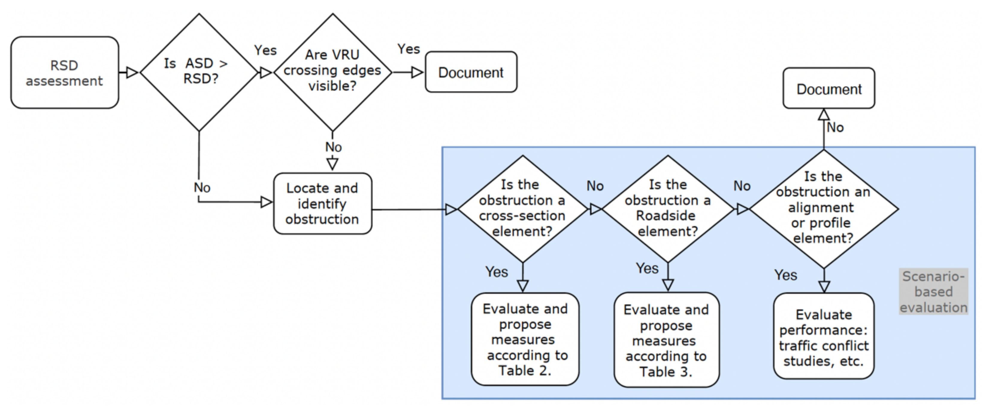
The procedure first determines the RSDs of the urban intersection; this is followed by the obtention of the ASDs and their subsequent comparison to the RSDs. After that, sightlines are launched towards the access points of vulnerable road users (VRUs) into the roadway. If these evaluations demonstrate that the road section has enough visibility, those stations that present values close to RSD thresholds are identified and documented. On the other hand, if the road section does not have enough ASDs, the obstruction is identified and located. Then, depending on the nature of the visual obstruction, a series of different actions are proposed. These actions entail the creation of scenarios. Finally, comparing the resulting scenarios allows the quantification of specific elements’ effects on visibility.
This procedure is summarized in Figure 1 and is described in subsequent sections.
This methodology is conducted virtually and requires updated and accurate depictions of the road scene. The 3D procedure uses 3D data inserted into a geographical information system (GIS) environment. A GIS procedure helps obtain and evaluate the ASD and facilitates its subsequent comparison to the RSD, as described by González-Gómez et al. [31,32]. The following sections illustrate the steps presented in Figure 1.
3.1.1. RSD Assessment
RSDs are definite lengths of roadway needed by road users to carry out specific maneuvers [4]. They are defined in several road guidelines of a wide variety of countries [4,15,33]. Intersections are complex road sections that require SSD and ISD [5]. RSDs can be calculated using equations or tables from road design guidelines [4,16,33,34]. RSDs are mainly impacted by the vehicle speed, deceleration rate, perception and reaction times, etc. Table 1 presents the standard equations to obtain SSDs and ISDs. These are taken from the Spanish road design standard and the design guidelines from the United States [4,16]. The different velocities are originally expressed as V, but numeric subscripts have been added to differentiate them. As there are different configurations of road intersections, the ISD equations presented are one specific type required for signalized legged intersections (for a road without priority). The parameter tg of Equation (4) is obtained using travel time behaviors obtained from field studies, information on the size of the geometry, vehicle sizes, and the speeds of intersecting legs.
3.1.2. Comparison of ASD and RSD
The ASD is mainly measured in order to be compared to the RSD. In that regard, the ASD has to be calculated considering the RSD that it will be compared to, as this will affect the height of both the observer and target, their placement on the lane, and the line of reference used to measure the distance. These parameters are also specified in road design guidelines and vary from one country to another [4,16]. After selecting the appropriate trajectories and eye heights for observers and targets, the next step is to model the road using one of the many available techniques. This study employs geospatial data, precisely, the LiDAR points obtained with a mobile mapping system (MMS). This dense point cloud is used to generate two models. One represents the road geometry and terrain, and the other represents the aboveground elements. Once the road is recreated, the procedure repeatedly launches lines-of-sight from the observer to the target using GIS tools [35] and calculates the ASD for each position.
SSDs are required in every section of the roadway and must be verified for every station. The value of the SSD remains constant for road sections that share the same speed, grade, and pavement conditions. The procedure carried out to determine the ASD needed for stopping produces tables with values of ASD for every considered station. Each value is then compared to the calculated SSD. As for the ISD, evaluations might vary depending on the type of intersection analyzed. In general, every intersection requires the definition of a decision point of which the ASD is to be compared to the ISD. This point is usually located on the approaches of those roads without priority [4].
With this methodology, ISD and SSD evaluations deliver the observer’s sightlines, consisting of unobstructed and obstructed ones. Obstructed lines of sight are divided into two—one from the observer to the obstruction and the other from the obstruction to the target. A point indicates the obstruction’s x, y, and z coordinates between them.
3.1.3. VRU Crossing Edges Verification
In addition to verifying if the ASD is of greater value than the RSD, it is crucial to confirm if drivers have a clear vision of the points where VRUs enter the roadway [36]. Verifying this condition is imperative on intersections where VRUs have the priority, but drivers need to detect their presence to yield.
Unlike the determination of sight distances (measured along the traveled way), the assessment of unobstructed visibility between a road user and a specific location, such as a conflict point or vertical signalization, can be performed using direct lines of sight [16]. For example, Figure 2 shows how parked vehicles could block the sightlines required for drivers to spot pedestrians about to cross.
3.1.4. Location and Categorization of Obstructions: Experiments
This step aims to assist in evaluating and handling obstructions detected in the previous sections. Additionally, it could be used to quantify or inspect the impact of specific objects or entities on visibility. The following assessments pay special attention to elements commonly found in urban environments, specifically, but not limited to, those found in Madrid, Spain. Examples of this are the trash containers, signs, and unkempt bushes presented in Figure 3.
Two categories of visual obstructions were created depending on their location. The first group contains those elements on the roadway, that is, on the lanes of the road and shoulders. The second group includes those elements located on the roadside. Profile or alignment elements could also obstruct the visibility, but their reformations are more complex, requiring in-depth evaluations, and therefore these are not considered in this study. This categorization is justified because elements blocking visibility could be within the roadway, next to it, or part of it.
- (a)
- Assessment of the impact of cross-section features on visibility
The roadway contains elements that ensure its proper functioning. These could be part of its signage, safety barriers, medians, channelization, landscaping, etc. Some of these elements are required at specific locations, but others could be removed, replaced, or relocated. Among the wide variety of components that could be present on a cross-section, some of those with a functionality that allows for their removal, relocation, or resizing are presented in Table 2 next to their proposed evaluation.
- (b)
- Assessment of the impact of roadside features on visibility
Roadsides are strips of land beside the road. These could contain facilities to accommodate pedestrians, riders, and cyclists. Furthermore, they serve many purposes and host functional elements of built-up areas, transportation, and public utilities. Table 3 contains elements commonly found on roadsides, which could block the sightlines required to provide reciprocal visibility between motorists and VRUs or obstruct SSDs in horizontal curves without proper clearance. This table lists them in addition to their proposed evaluation.
Once the proposed evaluation is selected, its modification could be simulated by adjusting the original component (creating a new scenario) and re-launching the assessment. After that, it is possible to compare the results obtained from the two scenarios (former and new). Equally, these modifications could be proposed to estimate and quantify the impact of specific features that do not necessarily block the RSD.
Examples of the experiments or evaluations that could be performed are:
- Impact of feature location on RSD/visibility (examining its relocation).
- Impact of feature size on RSD/visibility (examining its resizing or removal).
- Impact of feature type on RSD/visibility (examining its replacement or removal).
These evaluations are justified by the need to ensure that basic urban elements do not impact the visibility required by motorists, micromobility users, and pedestrians. Moreover, urban furniture elements have increased in size and number around numerous cities worldwide [37].
3.1.5. Scene Modeling
The GIS procedure previously described allows the obtention of the exact coordinates of the obstruction. The obstruction correction can be simulated within the GIS software ArcScene, and this modified model could be used to re-run the analysis. Object replacements and redesigns are made possible by importing 3D elements into the LiDAR-derived model. These 3D elements could be imported from the following formats: COLLADA (.dae), OpenFlight 15.8 (.flt), SketchUp 6.0 (.skp), 3ds Max (.3ds), or VRML 2.0 models (.wrl).
These 3D objects describing road and city furniture elements are nowadays more popular with the advent of digital twins or digital 3D city models, which are used for a wide variety of purposes [18]. 3D objects can be found online in 3D modeling software warehouses. They can also be modeled using these software suites. In that regard, most of the elements included in Table 2 and Table 3 describe regular geometries and could be modeled with relative ease. Conversely, vegetation is composed of heterogeneous elements, which poses some difficulties to its modeling. Moreover, plants, trees, and shrubs tend to change rapidly, adopting specific configurations due to wind, time of the year, etc. Fortunately, many 3D objects describing landscaping shrubs and plants commonly located in urban environs can be found online. Other elements that pose difficulties in their modeling are motor vehicles. Even though their fixed dimensions can be obtained from their manufacturers, they describe very complex geometries. These elements are commonly found in 3D warehouses as well.
3D urban elements are classified depending on their level of detail (LOD). This classification refers to their level of simplicity or thoroughness, and it ranges from 0 (two-dimensional footprint) to 4 (most detailed model) [18]. When evaluating elements that could cause obstructions, their LODs need not be higher than 3. Their dimensions must be the same as the objects, but they do not need color, texture, or semantic information. One such example is shown in Figure 4. This planter was modeled using the measurements specified by the city of Madrid, using the Solidworks program [19].
Lastly, the results derived from the scenarios are compared and evaluated to gain insights into their impact on visibility, to propose changes in the location or type of elements, etc.
3.1.6. Statistical Analysis
The results from the RSD assessments are presented in tables with detailed data on the sightlines launched from the observers to the targets. These tables display their length, visibility status (seen target or not), azimuth, etc. The size of each table will depend on the number of stations considered. If the lines are not obstructed, their total is determined through Equation (5):
where:
- Clear LOSn,m = the number of sightlines that are not obstructed.
- n = the total number of stations (observer stations plus target stations).
- m = the number of stations to be assessed (m = 2, observer and target stations).
As mentioned above, when the sightlines are obstructed, they are divided into two. Consequently, the total number of lines will increase depending on how many are blocked.
After verifying which scenario provides better results in terms of RSD adequacy (direct comparisons of those available and required), a statistical analysis is conducted to examine the lengths of the sightlines between observers and targets. The latter aims to evaluate and quantify the differences between them. In addition, this assessment aims to know if the visibility parameters are significantly different due to the presence of roadside or cross-section elements. The statistical model for these experiments is given in Equations (6)–(8):
with
where:
yijk describes the length of the lines of sight measured between a road user A at its ith position, and a road user B at its jth position (the target), considering the effect of the visual obstruction k, at a specific road intersection. µijk is the true mean of the line of sight from road user A at its ith position to road user B in its jth position. µ is the grand mean length of the lines of sight between a road user A at its ith position, and a road user B at its jth position, considering the effect of the visual obstruction k; αi is the main effect for a road user A at its ith position, βj is the main effect for the jth position of road user B; δk is the main effect of the kth obstruction; γijαβ is the interaction effect of road user A in position i and road user B at position j; γikαδ is the interaction effect of road user A in position i with the visual obstruction k; γjkβδ is the interaction effect of road user B in position j with the visual obstruction k. εijk is the random deviation, considered to have a normal distribution with constant variance for all samples considered. γijkαβδ is considered to be zero. Equation (9) shows the restrictions.
3.2. Case Study
These evaluations were performed at two intersections in the city of Madrid.
3.2.1. Locations
Intersection 1:
The first one is a circular intersection located in the university district. Figure 5 shows its aerial photography and layout. Three streets meet at this junction: Paseo de Juan XXIII, de la Sierra, and General Asensio Cabanillas. The main road, Paseo de Juan XXIII, is a two-way road with an average lane width of 3.4 m and flares on each approach that reach 7.5 m; its northbound approach is deflected. General Asensio Cabanillas St. is a one-way road; traffic could turn right towards Paseo de Juan XXIII or enter the circulatory roadway. De la Sierra St. is also a one-way road in which the traffic could come from the circulatory roadway or turning right from Paseo de Juan XXIII St. Their posted speed limits are 30 km/h. This yield-controlled intersection has two bus stops and channeling islands with landscaping bushes and vegetation in its surrounding areas.
On-street parking is allowed in the approaches of all three streets, on both sides. Figure 6 illustrates the approaches of Paseo de Juan XXIII St., where angled on-street parking is also allowed within the intersection area. Moreover, two bus stops and four pedestrian crossings are also contained within the intersection’s physical area.
Intersection 2:
The second intersection surveyed is a T-intersection where Obispo Trejo and Antonio Nebrija streets meet. Their posted limits are 30 km/h as well. This intersection is controlled with stop signs on the minor road, Antonio Nebrija St. These are illustrated in Figure 7.
On-street parking is allowed on the minor road on both sides, as shown in Figure 8.
Of the several elements that could obstruct the visibility of the intersections presented above, vegetation, vertical signalization, and on-street parking appeared to be the ones with a substantial impact.
3.2.2. Data Acquisition and Processing
The intersections presented in the previous section were surveyed the same day with an MMS. As mentioned in the literature review, several authors have employed MMS to acquire the data required to model the road and carry out sight distance estimations [19,38,39]. The MLS used was the IP-S3 from Topcon (Figure 9). This system integrates GNSS units (GPS and GLONASS) with an INS (inertial navigation system) and an odometer. Its sensor, a Velodyne HDL-32E, captures approximately 700,000 points per second. This sensor can provide a relative accuracy of ± 2 cm, reaching up to 100 m with a horizontal field of view (FOV) of 360° and a vertical FOV of +10° to −30°. It also includes a Ladybug 3 panoramic camera, with a 8000 × 4000 pixel resolution, and add-on imagery sensors [40].
This survey was planned and compiled to meet approximately ±10 mm horizontal and ±15 mm vertical accuracy at a 95% confidence level. GNSS observations were post-processed utilizing an external receiver located within 1.5 km of the intersections. As a result, the root-mean-square error of the trajectory had overall values lower than 8 cm.
The resulting point clouds were preprocessed in-house with software provided by the vendors. Subsequently, the point clouds of the whole survey were divided into files of 20,000,000 points in the LAS format. Then, denoizing, classification, and filtering were performed using MDTopX [41].
4. Results
The procedure introduced in the previous sections was applied to the road intersections presented in Section 3.2. The main insights obtained from these evaluations and the road simulations are presented herein.
4.1. RSD Assessment
The SSD was obtained with Equation (1). The values of most parameters are included in the guidelines. The SSD of both intersections employed their posted speed limits (30 km/h); the perception and reaction time used was the one stipulated in the guidelines (2.5 s); the deceleration rate was also the one included in the policies with a value of 3.4 m/s2. As both intersections were at-grade, the value of G was 0. The calculated SSD value was 31.79 m. Unlike the SSD, which was the same for both legs of the intersections analyzed, the ISD varied for each turn. Intersection 1 allows nine turns, and intersection 2 allows five. The results presented below show the most relevant ones in relation to visibility.
4.2. ASD vs. RSD and VRU’s Crossing Edges
The RSD-versus-ASD assessment confirmed that vegetation and on-street parking blocked the sightlines of various observers in both intersections. These findings supported the experiments described in the following sections, the results of which are organized based on the element that caused the obstruction, or element to be assessed, and the models created to obtain further insights for each intersection.
4.3. Scenarios Created for Intersections 1 and 2
Intersection 1 had populated shrubs on its cross-section (channeling islands). These shrubs did not block the RSD. Nonetheless, they were evaluated to assess what portion of the island could be filled with vegetation and which could not. With this in mind, three scenarios were created. The first one depicted the intersection as is, without modifications from its original state. The second one (scenario two) had the shrubs removed from the channeling island. Finally, the third one (scenario three) had the channeling islands filled with shrubs. Scenarios 1 to 3 were created for intersection 1.
Both intersections allowed on-street parking, which blocked the RSD of specific movements. Therefore, scenarios 4, 5, 6, 7, and 8 were created to evaluate potential solutions to this problem. Scenarios 4 and 5 were made for intersections 1 and 6; 7, and 8 were designed to model intersection 2. Scenario 4 depicted intersection 1 as is (with parked cars); scenario 5 had the car parked nearest the pedestrian crossing removed. Scenario 6 described intersection 2 as is, whereas scenario 7 also had parked vehicles near the pedestrian crossing removed; scenarios 8 and 9 replaced one of the parked cars with a van (Figure 10). The characteristics of the van were chosen using national car fleet statistics.
Lastly, scenarios from 10 (Figure 11) to 14 evaluated the impact of urban furniture elements on visibility. These were generated for intersection 2. They were created by filling the space of the removed parked cars with common urban furniture elements. Scenario 10 replaced the vehicle nearest to the pedestrian crossing of the intersection with trash containers; scenario 11 replaced it with a large flowerpot. Scenarios 12 to 14 changed the height of a hypothetical plant located inside the flowerpot.
Table 4 lists the scenarios created for both intersections; it summarizes each scenario’s aim and description.
4.4. Assessment of Scenarios
4.4.1. Impact of Vegetation on Visibility
This evaluation was carried out at intersection 1. It examined the effect of landscaping elements and verified whether the bushes present in the channeling island blocked drivers’ visibility on the circulatory roadway. In this evaluation, observers were located 1.5 m from the centerline, with an eye height of 1.1 m, as stipulated in the Spanish guidelines [16]. The evaluations were performed from the decision points of drivers inside the circulatory roadway (red dots in Figure 12) towards the conflicting trajectory, depicted with blue dots. The positions of both road users were also specified in the revised guidelines [16].
The bushes located in the channeling island were trimmed on the sides next to the roadway. The RSD assessment indicated that they did not block the sightlines of observers at the yield line. Still, they blocked those about to stop (drivers located a few meters before the yield line). Results showed that stations situated right at the yield line could see drivers traveling on Paseo Juan XXIII at distances longer than the SSD of 31.79 m. This evaluation was re-run, populating the channeling island with bushes. The results obtained from comparing scenarios 1 and 3 are presented in Figure 13.
The intermittent orange line depicts the visibility from the stations shown above, with the channeling island filled with vegetation (Scenario 3); the thinner red line shows the visibility of the intersection as is (Scenario 1). As shown in Figure 13, the differences in sight distances between scenarios 1 and 3 reached values up to 31 m. These results indicate the need to keep the bushes trimmed; otherwise, the visibility requirements will not be met.
The statistical evaluation described in Section 3.1.6 was carried out with the factors considered in this specific experiment. The model is analogous to Equation (6). In this case, yijk describes the length of the lines of sight measured between a road user merging into Paseo de Juan XXIII from the circulatory roadway (factor A) at its ith position (level), and a southbound driver along Paseo de Juan XXIII (factor B) at its jth position (level), in the presence of the number of bushes (factor C) at its kth level. The number of levels for factor A (I) was 14 (number of stations for the first driver), the number of levels for factor B (J) was 45 (number of stations for the second driver), and the number of levels for factor C (K) was two (real setting vs. increased vegetation). In this case, there were IJK populations, or “treatment combinations,” equal to 1260. Their restrictions are stated in Equation (9) with i from 1 to 14, j from 1 to 45, and k from 1 to 2.
The hypotheses were H0A: αi = 0 ∀i versus HaA: at least one αi ≠ 0; H0B: βj = 0 ∀J versus HaB: at least one βj ≠ 0; H0C: δk = 0 ∀k versus H0C: at least one δk ≠ 0.
Preliminary results showed statistical significance for all the factors considered. As expected, the positions of the road users (factors A and B) had a great impact on their resulting visibility. The effects of factor C (the obstruction) were further evaluated. Results are presented in Table 5. This shows the least-squares means differences using Student’s t distribution, differences in means, and confidence interval values. Table 5 highlights the small number that constitutes the differences between these two scenarios due to augmented vegetation. This table shows the least-square means of the visibility values of two scenarios through the differences in their means and the limits of their confidence intervals.
Despite being significantly different, the diminution in the length of the sightlines caused by the landscaping vegetation was expected to be higher.
4.4.2. Impact of On-Street Parking and Street Deflection on Visibility
This evaluation was carried out at intersection 1. As previously mentioned, the results showed that its northbound approach was deflected, and on-street parking was allowed on both sides. The RSD assessment highlighted that observers did not have enough SSD. These parked cars impacted the SSD because the deflection caused the sightlines to leave the roadway and enter it again, and the vehicles blocked them in the middle. In Figure 14 gray elements depict the vehicles, and the red dots indicate the locations where the sightlines were blocked (Scenario 4).
The evaluation also assumed that observers were located 1.5 m from the centerline with an eye height of 1.1 m and an object height of 0.5 m, as stipulated in the Spanish guidelines [16]. The car that caused the SSD insufficiency was removed (scenario 5). The model that governed this experiment is analogous to that described in Equation (6) and could be described as follows: yijk represents the length of the lines of sight measured between a northbound road user on Paseo de Juan XXIII at its ith position and their successive jth positions, considering the effect of the cars parked k. The number of levels for factor A (I) was 43 (number of stations for the observer), the number of levels for factor B (J) was 22 (number of successive stations along their trajectory), and the number of levels for factor C (K) was two (car vs. no car). In this case, there were IJK populations equal to 1892. Their restrictions are stated in Equation (9), with i ranging from 1 to 43, j from 1 to 22, and k from 1 to 2.
The hypotheses were H0A: αi = 0 ∀i versus HaA: at least one αi ≠ 0; H0B: βj = 0 ∀J versus HaB: at least one βj ≠ 0; H0C: δk = 0 ∀k versus H0C at least one δk ≠ 0.
The results showed statistical significance for the positioning (factors A and B). Factor C (presence of the car) was not significant to the response with a p-value of 0.2984. The least square means difference, evaluated with the Student’s t distribution, highlighted that levels were not significantly different (Table 6).
4.4.3. Impact of On-Street-Parking Element on Visibility: Type of Car Effect
This evaluation was carried out at intersection 2. Its RSD assessment and the estimation of the visibility towards the crossing edges highlighted that cars located at distances equal to the SSD and those at the intersection decision point could not spot pedestrians 1 m before the crossing. This evaluation considered drivers to be moving southbound from the minor road. The car causing the obstruction was removed to create an alternate scenario (scenario 7). Another scenario replaced the car with a van (scenario 8). The analysis was re-run with these three scenarios (6, 7, and 8).
As expected, the scenario with no car showed a higher number of unobstructed sightlines. Moreover, the van blocked the visibility of the edges of the pedestrian crossing to those drivers approaching the intersection.
The statistical comparison between the three scenarios was run as in the previous cases. The model was also analogous to the one introduced in Equation (6). It is detailed as follows: yijk describes the length of the lines of sight measured between a southbound road user in Nebrija St., at its ith position, and a pedestrian in the parallel sidewalk at its jth position, considering the effect of on-street parking k. The number of levels for factor i was 46, the number of levels for factor j was 76, and factor k had three levels. The number of treatment combinations was 10,488. Their restrictions are stated in Equation (9) with i ranging from 1 to 46, j from 1 to 76, and k from 1 to 3.
The hypotheses were analogous to the ones that governed the previous tests.
As in previous analyses, all factors and their interactions significantly affected the length of the sight distances. Equally, factors A and B (positions of observers and targets) showed higher differences among their levels than the differences caused by the obstructions. The effect of the obstacles was further evaluated using Tukey’s least square means differences (Table 7). All three levels were statistically different, again by small values. Their slight mean differences could be possibly caused by there being less than a dozen stations and the act that their sightlines were impacted by the presence of vehicles.
4.4.4. Impact of On-Street-Parking Element on Visibility: Side of the Street Effect
This evaluation was carried out at intersection 2. This evaluation examined which edge of the pedestrian crossing was most affected by on-street parking. As this street has one lane per direction, drivers along Nebrija St. are physically closer to pedestrians on their left. Still, their own vehicle’s bodywork does not impact their viewshed towards those on their right. This evaluation compares scenarios 8 (the van parked to the right of Nebrija St.) and scenario 9 (the van parked on the left of Nebrija St.). The RSD evaluation indicated that a vehicle blocks more sightlines when parked on the left.
The statistical evaluation defines yijk as the length of the lines of sight measured between southbound road users on Nebrija St., at its ith position, and pedestrians on the parallel sidewalk at its jth position, considering the effect of the side of the street where on-street parking is allowed k. The number of treatment combinations was 6992. Their restrictions are specified in Equation (9) with i from 1 to 46, j from 1 to 76, and k from 1 to 2.
The hypotheses were similar to those expressed in previous analyses. Here, all factors and interactions had a significant effect on the response. Factor C had the lowest impact, with a p-value of 0.0364. All other factors and interactions had p-values lower than 0.01. The Student’s t distribution was used to verify whether factor C levels differed significantly.
Table 8 shows that the side of the street where the car is parked has a significant effect on the lengths of the sightlines. However, the mean difference between both scenarios is lower than the other impacts investigated in previous sections.
4.4.5. Impact of Urban Furniture Elements on Visibility: Type of Element
This assessment was carried out at intersection 2. As highlighted in the previous evaluation, parked cars blocked the sightlines towards the pedestrian crossings. Hence, their removal would be beneficial to provide reciprocal visibility between pedestrians and motorists. However, it is common to find spaces where on-street parking is banned, filled with flower pots, trash containers, or other elements. These elements could enforce the ban because empty spaces could be used unlawfully. However, their presence could affect the required visibility. Therefore, the space cleared up by removing the car was filled with additional features commonly seen in cities to study these issues. The evaluations are detailed in the following sections.
Previous evaluations showed that removing the parked car helped to increase the visibility of intersection 2. With this in mind, and knowing that urban space is subject to many uses, the area that would be empty if a non-parking ban was enforced was filled with two trash containers with the exact dimensions as those presented in Figure 3; scenario 10 (Figure 11). Next, scenario 11 was created by filling the space with a large flowerpot that would prevent cars from parking.
The trash containers did block the visibility of the crossing edges when located in the center of the cleared spot. This result was expected because their height was higher than regular cars. On the other hand, the scenario containing an empty flower pot provided results similar to those with no car in it (this was also expected as its height was only 50 cm). As the empty flower pot did not differ from the results obtained with the empty scenario, the impact of trash containers was compared with the effects of a flower pot with a 30 cm-tall plant (scenario 12).
The statistical evaluation between scenarios 11 and 12 defines yijk as the length of the lines of sight measured between southbound road user on Nebrija St., at its ith position, and pedestrians on the parallel sidewalk at its jth position, considering the effect of the type of urban furniture element k. The number of treatment combinations was 6992. Their restrictions are analogous to those presented in Equation (9) with i from 1 to 46, j from 1 to 76, and k from 1 to 2.
The results showed that all factors and interactions were statistically significant, with p-values lower than 0.01. As before, the effects of the obstructions were analyzed using Student’s t distribution. Table 9 shows, as with previous cases, that the levels of factor C were significantly different by a marginal value.
4.4.6. Impact of Urban Furniture Elements on Visibility: Different Element Sizes
This evaluation was also carried out at intersection 2. As the previous assessment highlighted that the empty flowerpot did not affect visibility, new scenarios were created considering plants with different heights on the flowerpot. The considered sizes were 30 cm, 60 cm, and 90 cm. The results of their RSD assessments are presented in Figure 15. The flowers of 30 cm and 60 cm (scenarios 12 and 13, respectively) provided the same ASD values and are represented by the red dotted line. However, scenario 14, which contained the 90 cm-high shrub, showed lower visibility (intermittent green line).
This type of evaluation could be helpful in establishing a limit on the allowed growth of landscaping elements. In this case study, the differences in sight distances due to the height of the plants were around 10 m.
This statistical evaluation for this case defines yijk as the length of the lines of sight measured between a southbound road user on Nebrija St., at its ith position, and pedestrians on the parallel sidewalk at its jth position, considering the effect of the height of the plant inside the flower pot k. The number of levels for factor i was 46, the number of levels for factor j was 76, and factor k had three levels. The number of treatment combinations was 10,488. Their restrictions are analogous to those presented in Equation (9) with i from 1 to 46, j from 1 to 76, and k from 1 to 3. The hypotheses were similar to those expressed in previous analyses.
Factors A, B, and C were significant. Interactions that considered the effect of the positions of observers and targets (A * B) and the position of the observer and the height of the obstacle (A * C) were also significant. The interaction of the target’s position (the pedestrian) and the obstacle’s size was not significant, with a p-value of 0.5478. A further evaluation of the effects of plant height confirmed that levels 2 and 1 were not statistically different (plants with heights of 30 cm and 60 cm). However, level 3 (plant with a height of 90 cm) was significantly different from the other two, similarly to the results obtained in the RSD assessment.
5. Conclusions
This paper presented a modeling-based methodology for assessing the impact of typical visibility-obstructing elements. Visual obstructions found in this study were common elements found in urban settings. The capability of creating scenarios allowed the evaluation of the impact of those elements on visibility. A rigorous statistical assessment and the sight distance evaluation helped to quantify these effects considering all road users and their multiple locations.
The size and type of shrubs present in intersection 1 did not affect the visibility of drivers stopped at the yield line. However, when shrubs of the same size filled the island, the visibility was blocked. The difference in width between the two was less than 2 m. This assessment demonstrates the importance of specific thresholds of areas to be kept clear in channeling islands, medians, etc.
Evaluating the visibility effects of on-street parking highlighted that some areas require the regulation of parking near pedestrian crossings. Drivers need to see pedestrians in order to yield, and vehicles of large dimensions might block the pedestrian crossing entry. For instance, cities with high parking demand could assess which intersections provide enough visibility for pedestrians, which intersections should not allow ample vehicles to park near pedestrian crossings, and which side of the pedestrian crossing is less visible. This procedure allowed us to evaluate these aspects and quantify the impact of each of these measures objectively.
In addition to on-street parking, city elements such as garbage bins, information panels, and others are usually placed within the functional areas of intersections. These elements are usually placed with no regard to their impact on visibility. As the evaluation highlighted, tall trash containers had an even worse impact on visibility than on-street parking. Consequently, their location should also be regulated and kept out of the entrances of pedestrian crossings.
This study includes some assumptions related to the obtention of the required and available sight distances. They were based on standards and official guidelines. The evaluation of how these assumptions could impact the results will be part of future lines of research. Furthermore, future work will include intersections with more complex geometries and more lanes in order to analyze the relationship between the methodology’s performance and the intersection’s complexity.
Author Contributions
Conceptualization, M.C.; methodology, M.C., D.K.R., and K.G.-G.; software D.K.R. and K.G.-G.; formal analysis, M.C., D.K.R., and K.G.-G.; investigation, M.C. and K.G.-G.; resources, M.C.; writing—original draft preparation, M.C., D.K.R., and K.G.-G.; writing—review and editing, M.C., D.K.R., and K.G.-G.; supervision, M.C.; project administration, MC; funding acquisition, M.C. All authors have read and agreed to the published version of the manuscript.
Funding
This research was funded by the Spanish Ministerio de Economía y Competitividad and the European Regional Development Fund (FEDER), grant number TRA-2015-63579-R (MINECO/FEDER).
Institutional Review Board Statement
Not applicable.
Informed Consent Statement
Not applicable.
Data Availability Statement
Data are not available because they are proprietary.
Conflicts of Interest
The authors declare that they have no conflict of interest. The funders had no role in the study design, in the collection, analyses, or interpretation of data, in the writing of the manuscript, or in the decision to publish the results.
References
- Miranda-Moreno, L.F.; Morency, P.; El-Geneidy, A.M. The link between built environment, pedestrian activity and pedestrian–vehicle collision occurrence at signalized intersections. Accid. Anal. Prev. 2011, 43, 1624–1634. [Google Scholar] [CrossRef] [PubMed]
- Connolly, P.L.; Marcus, K.H. Human and Visual Factors Considerations for the Design of Automotive Periscopic Rear Vision Systems. SAE Trans. 1968, 77, 1346–1364. [Google Scholar]
- Hristov, B. Influence of Road Geometry on Driver’s Gaze Behavior on Motorways. E3S Web Conf. 2019, 97, 01001. [Google Scholar] [CrossRef]
- AASHTO. A Policy on Geometric Design of Highways and Streets, 8th ed.; AASHTO: Washington, DC, USA, 2018; ISBN 9781560516767. [Google Scholar]
- Ministerio de Fomento. Guía de Nudos Viarios; Ministerio de Fomento: Madrid, Spain, 2012. [Google Scholar]
- Kraemer, C.; Pardillo, J.M.; Rocci, S.; Romana, M.G. Ingeniería de Carreteras. Volumen I, 2nd ed.; Concepción Fernandez, Ed.; McGraw-Hill Interamericana: Madrid, Spain, 2003; ISBN 8448139887. [Google Scholar]
- Moretti, L.; Palazzi, F.; Cantisani, G. Operating Times and Users’ Behavior at Urban Road Intersections. Sustainability 2020, 12, 4120. [Google Scholar] [CrossRef]
- Underwood, G.; Chapman, P.; Bowden, K.; Crundall, D. Visual search while driving: Skill and awareness during inspection of the scene. Transp. Res. Part F Traffic Psychol. Behav. 2002, 5, 87–97. [Google Scholar] [CrossRef]
- James, O.; Swiderski, J.; Hicks, J.; Teoman, D.; Buehler, R. Pedestrians and E-Scooters: An Initial Look at E-Scooter Parking and Perceptions by Riders and Non-Riders. Sustainability 2019, 11, 5591. [Google Scholar] [CrossRef] [Green Version]
- Ma, Y.; Zheng, Y.; Easa, S.; Wong, Y.D.; El-Basyouny, K. Virtual analysis of urban road visibility using mobile laser scanning data and deep learning. Autom. Constr. 2022, 133, 104014. [Google Scholar] [CrossRef]
- Bassani, M.; Grasso, N.; Piras, M.; Catani, L. Estimating the Available Sight Distance in the Urban Environment by GIS and Numerical Computing Codes. ISPRS Int. J. Geo-Inf. 2019, 8, 69. [Google Scholar] [CrossRef] [Green Version]
- Gargoum, S.A.; Karsten, L. Virtual assessment of sight distance limitations using LiDAR technology: Automated obstruction detection and classification. Autom. Constr. 2021, 125, 103579. [Google Scholar] [CrossRef]
- Adminaité-Fodor, D.; Jost, G. Safer Roads, Safer Cities: How to Improve Urban Road Safety in the EU; European Transport Safety Council: Brussels, Belgium, 2019. [Google Scholar]
- DGT Accidentes Trafico Zona Urbana. Available online: http://www.dgt.es/es/seguridad-vial/estadisticas-e-indicadores/publicaciones/accidentes-urban/ (accessed on 10 October 2019).
- Austroads. Guide to Road Design Part 3: Geometric Design; Austroads Ltd.: Sydney, Australia, 2016; ISBN 978-1-922382-00-9. [Google Scholar]
- Ministerio de Fomento. Norma 3.1-IC: Trazado; Ministerio de Fomento: Madrid, Spain, 2016; ISBN 9788578110796.
- Jung, J.; Olsen, M.J.; Hurwitz, D.S.; Kashani, A.G.; Buker, K. 3D virtual intersection sight distance analysis using lidar data. Transp. Res. Part C Emerg. Technol. 2018, 86, 563–579. [Google Scholar] [CrossRef]
- Ma, Y.; Zheng, Y.; Cheng, J.; Zhang, Y. Hybrid Model for Realistic and Efficient Estimation of Highway Sight Distance Using Airborne LiDAR Data. J. Comput. Civ. Eng. 2019, 33, 04019039. [Google Scholar] [CrossRef]
- Ma, Y.; Zheng, Y.; Cheng, J.; Easa, S. Real-Time Visualization Method for Estimating 3D Highway Sight Distance Using LiDAR Data. J. Transp. Eng. Part A Syst. 2019, 145, 04019006. [Google Scholar] [CrossRef]
- Guan, H.; Li, J.; Cao, S.; Yu, Y. Use of mobile LiDAR in road information inventory: A review. Int. J. Image Data Fusion 2016, 7, 219–242. [Google Scholar] [CrossRef]
- Pappalardo, G.; Cafiso, S.; Di Graziano, A.; Severino, A. Decision Tree Method to Analyze the Performance of Lane Support Systems. Sustainability 2021, 13, 846. [Google Scholar] [CrossRef]
- Olsen, M.J.; Roe, G.V.; Glennie, C.; Persi, F.; Reedy, M.; Hurwitz, D.; Williams, K.; Tuss, H.; Squellati, A.; Knodler, M. Guidelines for the Use of Mobile LIDAR in Transportation Applications; National Cooperative Highway Research Program (NCHRP) Report 748; Transportation Research Board: Washington, DC, USA, 2013. [Google Scholar]
- Khattak, A.J.; Shamayleh, H. Highway Safety Assessment through Geographic Information System-Based Data Visualization. J. Comput. Civ. Eng. 2005, 19, 407–411. [Google Scholar] [CrossRef]
- Zariņš, A.; Naudžuns, J.; Ing, S.; Kaļinka, M.; Smirnovs, J. Sight Distance detection using LIDAR and GPS data Bearing Capacity Assessment on low Volume Roads View project Sight Distance detection using LIDAR and GPS data. In Proceedings of the Transport Research Arena Europe, Brussels, Belgium, 7–10 June 2010; p. 8. [Google Scholar]
- Tarel, J.P.; Charbonnier, P.; Goulette, F.; Deschaud, J.E. 3D road environment modeling applied to visibility mapping: An experimental comparison. In Proceedings of the 2012 IEEE/ACM 16th International Symposium on Distributed Simulation and Real Time Applications, Dublin, Ireland, 25–27 October 2012; pp. 19–26. [Google Scholar] [CrossRef] [Green Version]
- Khattak, A.; Hallmark, S.; Souleyrette, R. Application of Light Detection and Ranging Technology to Highway Safety. Transp. Res. Rec. J. Transp. Res. Board 2003, 1836, 7–15. [Google Scholar] [CrossRef]
- Tsai, Y.; Yang, Q.; Wu, Y. Use of Light Detection and Ranging Data to Identify and Quantify Intersection Obstruction and Its Severity. Transp. Res. Rec. J. Transp. Res. Board 2011, 2241, 99–108. [Google Scholar] [CrossRef]
- Olsen, M.J.; Hurwitz, D.; Kashani, A.; Buker, K. 3D Virtual Sight Distance Analysis Using Lidar Data; Pacific Northwest Transportation Consortium (PacTrans): Washington, DC, USA, 2016. [Google Scholar]
- De Santos-Berbel, C.; González-Gómez, K.; Castro, M.; Anta, J.A.; de Santos Berbel, C.; González Gómez, K.; Anta, J.A. Addressing sight-distance-related safety effects of installing median barriers at horizontal curves of undivided highways under a 3D approach. In Proceedings of the 5th International Conference on Road and Rail Infrastructure, Zadar, Croatia, 17–19 May 2018; pp. 1067–1073. [Google Scholar] [CrossRef] [Green Version]
- Gonzalez-Gomez, K.; Iglesias, L.; Rodriguez-Solano, R.; Castro, M. Evaluating 3-D Sight Distance at Urban Intersections Using a LiDAR-Based Model and Considering Multiple Users. In Proceedings of the International Conference on Traffic and Transport Engineering (ICTTE 2018), Belgrade, Serbia, 27–28 September 2018; Cokorilo, O., Ed.; City Net Scien Res Ctr Ltd-Belgrade: Belgrade, Serbia, 2018; pp. 765–772. [Google Scholar]
- González-Gómez, K.; Iglesias, L.; Rodríguez-Solano, R.; Castro, M. Framework for 3D Point Cloud Modelling Aimed at Road Sight Distance Estimations. Remote Sens. 2019, 11, 2730. [Google Scholar] [CrossRef] [Green Version]
- González-Gómez, K.; Castro, M. Evaluating Pedestrians’ Safety on Urban Intersections: A Visibility Analysis. Sustainability 2019, 11, 6630. [Google Scholar] [CrossRef] [Green Version]
- Ministero delle Infrastrutture e dei Trasporti. Norme Funzionali e Geometriche per la Costruzione Delle Strade; Ministero delle Infrastrutture e dei Trasporti: Roma, Italy, 2001.
- Austroads Ltd. Guide to Road Design: Part 4A: Unsignalised and Signalised Intersections, 3rd ed.; Austroads Ltd.: Sydney, Australia, 2017; ISBN 978-1-925451-73-3. [Google Scholar]
- Iglesias, L.; Castro, M.; Pascual Gallego, V.; de Santos-Berbel, C. Estimation of sight distance on highways with overhanging elements. In Proceedings of the International Conference on Traffic and Transportation Engineering 2016, Belgrade, Serbia, 24–25 November 2016. [Google Scholar]
- AASHTO. Guide for the Development of Bicycle Facilities, 4th ed.; AASHTO: Washington DC, USA, 2012. [Google Scholar]
- Fitzpatrick, K.; Wooldridge, M.D.; Blaschke, J.D. Urban Intersection Design Guide: Volume 1 Guidelines; Texas A&M Transportation Institute: Austin, TX, USA, 2005. [Google Scholar]
- González-Jorge, H.; Díaz-Vilariño, L.; Lorenzo, H.; Arias, P. Evaluation of driver visibility from mobile lidar data and weather conditions. Int. Arch. Photogramm. Remote Sens. Spat. Inf. Sci. ISPRS Arch. 2016, 2016, 577–582. [Google Scholar] [CrossRef] [Green Version]
- Castro, M.; Lopez-Cuervo, S.; Paréns-González, M.; de Santos-Berbel, C. LIDAR-based roadway and roadside modelling for sight distance studies. Surv. Rev. 2016, 48, 309–315. [Google Scholar] [CrossRef]
- Topcon Positioning Systems IP-S3. Specifications. Available online: https://www.topconpositioning.com/en-na/mass-data-and-volume-collection/mobile-mapping/ip-s3 (accessed on 25 February 2018).
- Digi21 Modelos Digitales Topográficos MDTopX. Available online: https://www.digi21.net/MDTop (accessed on 14 June 2018).
Figure 1.
Depiction of the proposed procedure.

Figure 2.
Sightline blocked by on-street parked traffic.

Figure 3.
Elements commonly found in urban settings (a) urban furniture; (b) unkempt vegetation.

Figure 4.
Modeling the planter: (a) modeling the base; (b) real element.

Figure 5.
Intersection Paseo Juan XXIII, De la Sierra St. and General Asensio Cabanillas St.: (a) aerial photograph, (b) geometrical depiction.
Figure 5.
Intersection Paseo Juan XXIII, De la Sierra St. and General Asensio Cabanillas St.: (a) aerial photograph, (b) geometrical depiction.

Figure 6.
On-street parking along the intersection.

Figure 7.
Obispo Trejo and Antonio Nebrija St. intersection: (a) aerial photograph, (b) geometrical depiction.
Figure 7.
Obispo Trejo and Antonio Nebrija St. intersection: (a) aerial photograph, (b) geometrical depiction.

Figure 8.
Photograph of intersection 2.

Figure 9.
IP-S3 system from Topcon.

Figure 10.
Scenario 8.

Figure 11.
Two trash containers were used in scenario 10.

Figure 12.
Observers positioned along the circulatory roadway of the intersection.

Figure 13.
Comparison of real scenario (scenario 1) with one increasing the landscaping vegetation (scenario 3). These distances were measured along the roadway.
Figure 13.
Comparison of real scenario (scenario 1) with one increasing the landscaping vegetation (scenario 3). These distances were measured along the roadway.

Figure 14.
Parked cars on the intersection approach (scenario 4).

Figure 15.
Results of the scenarios with flowerpots of different heights. In red, scenarios 12 and 13 (plant heights of 30 and 60 cm, respectively); scenario 14 (plant height of 90 cm) in green.
Figure 15.
Results of the scenarios with flowerpots of different heights. In red, scenarios 12 and 13 (plant heights of 30 and 60 cm, respectively); scenario 14 (plant height of 90 cm) in green.


Table 1.
Equations to obtain the SSD and ISD according to guidelines from Spain and the United States (USA).
Table 1.
Equations to obtain the SSD and ISD according to guidelines from Spain and the United States (USA).
| Country | SSD Equations (1) and (3) | ISD Equations (2) and (4) |
|---|---|---|
| Spain [1,2] | (1) where: Dp = stopping sight distance (m). V1 = speed at the starting time of the stopping maneuver (km/h). tp = perception and reaction time (s). fl = coefficient of friction between the road surface and the tire. i = the slope (m/m). | (2) where: Dc = the crossing distance (m). V2 = the speed in the intersecting road (km/h). tc = the time it takes for the intersecting vehicle to complete the crossing maneuver (s). |
| USA [3,4] | (3) where: SSD = stopping sight distance (m). Vd = design speed (km/h). t = brake reaction time (s). a = deceleration rate (m/s2). G = slope (m/m) | (4) where: ISD = Intersection sight distance (m). Vmajor = the speed in the major road (km/h). tg = time gap for minor road drivers to enter a major road (s). |
Table 2.
Proposed treatment for visibility-obstructing cross-section elements.
| Type | Element | Proposed Evaluation |
|---|---|---|
| City planning | On-street parking, Trash containers, | Simulate removal of a few spots. Simulate removal or change of size/type |
| Road safety | Bikeway segregating element | Simulate change of size/type. |
| Median, strip landscaping | Simulate modification, replacing. | |
| Signage | Simulate slight relocation. |
Table 3.
Proposed treatment for visibility-obstructing roadside elements.
| Type | Elements | Proposed Evaluation |
|---|---|---|
| Public transit furniture | Bus stops, ticketing machines, information panels. | Simulate relocation, replacement, or redesign. |
| Urban furniture | Maildrop, benches, trash containers. | |
| Vegetation | Trees, bushes, landscaping |
Table 4.
Scenarios created with their description and purpose.
| Scenario | Intersection | Description | Aim |
|---|---|---|---|
| 1 | 1 | As is. | Real scenario for intersection 1. Reference for comparisons. |
| 2 | 1 | Removal of vegetation. | Impact of vegetation on visibility. |
| 3 | 1 | Modification of vegetation. | Impact of vegetation on visibility. |
| 4 | 1 | As is (with parked cars). | Real scenario for intersection 1. Reference for comparisons. |
| 5 | 1 | Without parked cars (removal of automobiles parked near pedestrian crossings). | Impact of on-street parking on visibility. |
| 6 | 2 | As is (with parked cars). | Real scenario for intersection 2. Reference for comparisons. |
| 7 | 2 | Without parked cars (removal of automobiles parked near pedestrian crossings). | Impact of on-street-parking element on visibility. |
| 8 | 2 | With parked van to the left. | Impact of on-street-parking element on visibility: type of car effect. |
| 9 | 2 | With a parked van to the right. | Impact of on-street-parking element on visibility: side of the street effect. |
| 10 | 2 | With trash containers. | Impact of urban furniture elements on visibility. |
| 11 | 2 | With a sizeable empty flowerpot. | Impact of urban furniture elements on visibility. |
| 12 | 2 | With 30 cm of plants above the large flowerpot. | Impact of the size of urban furniture elements on visibility. |
| 13 | 2 | With 60 cm of plants above the large flowerpot. | Impact of the size of urban furniture elements on visibility. |
| 14 | 2 | With 90 cm of plants above the large flowerpot. | Impact of the size of urban furniture elements on visibility |
Table 5.
Least square differences Student’s t for scenarios 1 and 3.
| Least Square Mean (visibility of scenario 1 (i)) | Least Square Mean (Visibility of Scenario 3(j)) | ||
| Mean(i) − Mean(j) | 1 | 2 | |
| Lower Confidence Level Difference | |||
| Upper Confidence Level Difference | |||
| 1 | 0 | 1.39946 | |
| 0 | 1.13676 | ||
| 0 | 1.66217 | ||
| 2 | −1.3995 | 0 | |
| −1.6622 | 0 | ||
| −1.1368 | 0 | ||
Table 6.
Least square differences (Student’s t) for scenarios 4 and 5.
| Least Square Mean (visibility of scenario 4 (i)) | Least Square Mean (Visibility of Scenario 5 (j)) | ||
| Mean(i) – Mean(j) | 1 | 2 | |
| Lower Confidence Level Difference | |||
| Upper Confidence Level Difference | |||
| 1 | 0 | −0.8709 | |
| 0 | −2.513 | ||
| 0 | 0.77125 | ||
| 2 | 0.87089 | 0 | |
| −0.7713 | 0 | ||
| 2.51302 | 0 | ||
Table 7.
Least square means differences using Tukey’s honest significant differences for scenarios 6, 7, and 8.
Table 7.
Least square means differences using Tukey’s honest significant differences for scenarios 6, 7, and 8.
| LSMean(i) | LSMean[j] | |||
| Mean(i) – Mean(j) | 1 | 2 | 3 | |
| Lower Confidence Level Difference | ||||
| Upper Confidence Level Difference | ||||
| 1 | 0 | −0.3044 | 0.67698 | |
| 0 | −0.4013 | 0.58008 | ||
| 0 | −0.2075 | 0.77389 | ||
| 2 | 0.30442 | 0 | 0.9814 | |
| 0.20751 | 0 | 0.8845 | ||
| 0.40133 | 0 | 1.07831 | ||
| 3 | −0.677 | −0.9814 | 0 | |
| −0.7739 | −1.0783 | 0 | ||
| −0.5801 | −0.8845 | 0 | ||
Table 8.
Least square differences (Student’s t) for scenarios 8 and 9.
| Least Square Mean (visibility of scenario 8 (i)) | Least Square Mean (Visibility of Scenario 9 (j)) | ||
| Mean(i) − Mean(j) | 1 | 2 | |
| Lower Confidence Level Difference | |||
| Upper Confidence Level Difference | |||
| 1 | 0 | −0.1405 | |
| 0 | −0.2722 | ||
| 0 | −0.0089 | ||
| 2 | 0.14053 | 0 | |
| 0.00888 | 0 | ||
| 0.27217 | 0 | ||
Table 9.
Least square differences (Student’s t) for scenarios 11 and 12.
| Least Square Mean (visibility of scenario 11(i)) | Least Square Mean (Visibility of Scenario 12(j)) | ||
| Mean(i) – Mean(j) | 1 | 2 | |
| Lower Confidence Level Difference | |||
| Upper Confidence Level Difference | |||
| 1 | 0 | −0.4985 | |
| 0 | −0.5654 | ||
| 0 | −0.4316 | ||
| 2 | 0.49846 | 0 | |
| 0.43157 | 0 | ||
| 0.56536 | 0 | ||
Publisher’s Note: MDPI stays neutral with regard to jurisdictional claims in published maps and institutional affiliations. |
© 2021 by the authors. Licensee MDPI, Basel, Switzerland. This article is an open access article distributed under the terms and conditions of the Creative Commons Attribution (CC BY) license (https://creativecommons.org/licenses/by/4.0/).
Share and Cite
MDPI and ACS Style
González-Gómez, K.; Rollins, D.K.; Castro, M. Modeling Urban Road Scenarios to Evaluate Intersection Visibility. Sustainability 2022, 14, 354. https://0-doi-org.brum.beds.ac.uk/10.3390/su14010354
AMA Style
González-Gómez K, Rollins DK, Castro M. Modeling Urban Road Scenarios to Evaluate Intersection Visibility. Sustainability. 2022; 14(1):354. https://0-doi-org.brum.beds.ac.uk/10.3390/su14010354
Chicago/Turabian StyleGonzález-Gómez, Keila, Derrick K. Rollins, and María Castro. 2022. "Modeling Urban Road Scenarios to Evaluate Intersection Visibility" Sustainability 14, no. 1: 354. https://0-doi-org.brum.beds.ac.uk/10.3390/su14010354
Note that from the first issue of 2016, this journal uses article numbers instead of page numbers. See further details here.