
An MFD Construction Method Considering Multi-Source Data Reliability for Urban Road Networks


1
School of Traffic &Transportation Engineering, Xinjiang University, Hua Rui Street #777, Urumqi 830017, China
2
Intelligent Transportation System Research Center, Southeast University, Southeast University Road #2, Nanjing 211189, China
*
Author to whom correspondence should be addressed.
Sustainability 2022, 14(10), 6188; https://0-doi-org.brum.beds.ac.uk/10.3390/su14106188
Submission received: 15 April 2022
/
Revised: 17 May 2022
/
Accepted: 17 May 2022
/
Published: 19 May 2022
(This article belongs to the Special Issue Intelligent Mobility: Technologies, Applications and Services)
Abstract
:Road network traffic management and control are the key mechanisms to alleviate urban traffic congestion. With this study, we aimed to characterize the traffic flow state of urban road networks using the Macroscopic Fundamental Diagram (MFD) to support area traffic control. The core property of an MFD is that the network flow is maximized when network traffic stays at an optimal accumulation state. The property can be used to optimize the temporal and spatial distribution of traffic flow with applications such as gating control. MFD construction is the basis of these MFD-based applications. Although many studies have been conducted to construct MFDs, few studies are dedicated to improving the accuracy considering the reliability of different sources of data. To this end, we propose an MFD construction method using multi-source data based on Dempster–Shafer evidence (DS evidence) theory considering the reliability of different data sources. First, the MFD was constructed using VTD and CSD, separately. Then, the fused MFD was derived by quantifying the reliability of different sources of data for each MFD parameter based on DS evidence theory. The results under real data and simulated data show that the accuracy of the constructed MFDs was greatly improved considering the reliability of different data sources (the maximum MFD estimation error was reduced by 22.3%). The proposed method has the potential to support the evaluation of traffic operations and the optimization of signal control schemes for urban traffic networks.
1. Introduction
Road network traffic management and control based on the traffic supply–demand relationship are important means to actively alleviate urban traffic congestion and improve the operational efficiency of road traffic systems. Characterizing the traffic flow state of urban road networks is a fundamental problem to understand the traffic supply–demand relationship. In this study, we characterize the traffic flow state of urban road networks using the Macroscopic Fundamental Diagram (MFD), which has the following advantages: it can dynamically describe the traffic state of the road network, and it can be readily obtained with traffic flow data from existing detectors, etc. The existence of MFD has been confirmed in many cities around the world [1]. The core property of MFD is that the network traffic flow is maximized when network traffic stays at an optimal accumulation state (the network traffic flow remains maximum with increasing network traffic density). The property can be applied in gating control, traffic safety, congestion tolls, etc. [2,3,4,5,6]. The construction of an MFD is the basis of MFD-based applications.
Generally, there are three types of data to construct MFDs: cross-sectional data of traffic flow (CSD), vehicle trajectory data (VTD), and both sources of data. The general method to construct an MFD is the weighted average method for CSD and Edie’s method for VTD. However, MFD construction based on CSD is greatly affected by the location of detectors, and that based on VTD has high requirements for the penetration rate and the balanced spatial distribution of probe vehicles. Few multi-source data-based methods consider the different reliability of different sources of data, and the method that estimates different parameters of MFD with different data sources may lead to inconsistencies between the two parameters. In view of this, an MFD fusion method that can take advantage of different sources of data is needed.
Considering the different reliability of estimating ATF and ATD using CSD and VTD, we developed an MFD construction method based on the Dempster–Shafer evidence (DS evidence) theory using multi-source data. Firstly, the MFDs based on CSD and VTD were constructed separately. Secondly, the weight of CSD and VTD for ATF and ATD were separately estimated using DS evidence theory, and then the fusion MFD was derived and evaluated. The proposed method aims to improve the accuracy of MFD construction by making full use of different sources of data. To this end, the contributions of this paper can be described as follows: (1) an MFD construction method was proposed considering the difference in penetration of probe vehicles with different origins and destinations (OD); (2) a fusion method for MFD construction was proposed considering the different reliability of different sources of data.
2. Literature Review
The construction of an MFD is the basis of MFD-based applications. Regarding the different data sources, three types of data were included for MFD construction: cross-sectional data of traffic flow (CSD), vehicle trajectory data (VTD), and both sources of data. The studies on MFD construction are introduced as follows.
MFD construction based on CSD (such as loop detector data, microwave vehicle detector) derives the average traffic density (ATD) and average traffic flow (ATF) of the road network through aggregating links’ traffic density and traffic flow. Geroliminis and Daganzo [1] used loops and microwave detectors to detect traffic flow and occupancy, and derived the road network MFD considering the length of links. Limited by the cost of detector deployment, a cross-sectional vehicle detector is usually fragmented in the road network. How to detect cross-sectional traffic flow based on spatially fragmented vehicle detectors, and thus accurately construct an MFD, has become a problem that must be solved. In response to this problem, Ortigosa and Menendez [7] sought to find the optimal link combination by minimizing the difference of MFD derived from traffic flow data aggregated by partial links and all links based on VISSIM simulation; their results show that 25% of vehicle detectors can make the difference less than 15%.
However, the location of the cross-sectional vehicle detector has a significant impact on the estimation of ATD. Buisson and Ladier [8] divided the CSD into three categories according to the distance between the detector and the downstream signalized intersections, and then constructed MFD using the three types of data. They found that the closer the detector is to the downstream signalized intersections, the higher the slope of the rising section of the MFD obtained by these detectors. Courbon and Leclercq [9] conducted a comparative analysis of MFD construction based on VTD and CSD, and found that the accuracy of a constructed MFD depends on the distribution of loop detectors in the road network. Leclercq [10] pointed out that only using CSD to construct an MFD leads to inaccuracy, as the CSD cannot accurately capture the average traffic speed or density. In addition, Leclercq believes that the accuracy of MFD construction is significantly improved when estimating traffic flow using CSD and estimating traffic speed using VTD compared with the single use of the loop detector data. Tilg et al. [11] systematically evaluated two main analytical approximation methods to derive the MFD for arterial roads and urban networks, and the results revealed that the availability of signal data can improve the analytical approximation of the MFD.
The MFD construction using VTD is generally obtained by expanding the travel time and travel distance of probe vehicles, and the estimation of the penetration rate has to depend on CSD. Earlier studies assumed that the probe vehicles were evenly distributed in a road network. Geroliminis and Daganzo [1] used the position coordinates provided by taxis’ GPS, along with the effective travel information of the taxis to estimate the effective travel time and travel distance, and the CSD was used to estimate the taxis’ penetration rate. Nagle and Gayah [12] assumed that the probe vehicles’ penetration rate was constant among all OD pairs, using the probe vehicles’ proportion at fixed vehicle detectors to approximately estimate the penetration rate. Ambühl and Menendez [13] assumed that the loop detectors are evenly distributed in different positions of links, and constructed MFD with CSD and VTD; their results showed that the error of the constructed MFD was smaller for multi-source data than that of single-source data. In addition, the study also analyzed MFD construction errors under different penetration rates and loop detectors’ coverage rates. Considering the different penetration rate among different ODs, some scholars proposed new methods that can improve the rationality of MFD construction [14,15,16,17,18,19]. Du et al. [14] proposed a weighted average penetration rate estimation method for OD pairs based on fixed vehicle detectors and taxi GPS data. The simulation results show that the accuracy of the proposed method is higher than that of the unified penetration rate.
With the development of traffic detection technology, the coverage rate of fixed vehicle detectors and the penetration rate of probe vehicles on the urban roads have been significantly improved. Considering the characteristics of different data sources, some scholars proposed to estimate different parameters of MFD with different sources of data. Leclercq [10] pointed out that the accuracy of a constructed MFD will be greatly improved by using loop detector data to estimate ATF and by using VTD to estimate ATD, compared to using loop detector data to construct an MFD. Ji et al. [20] proposed to use CSD to estimate ATF, and use VTD to estimate the ATD. The accuracy of constructed MFDs using multi-source data has been improved. However, most of the studies assumed that the penetration rate was evenly distributed around the road network. A summary of the data type, data source, and the MFD construction methods of representative research is given in Table 1.
3. Materials and Methods
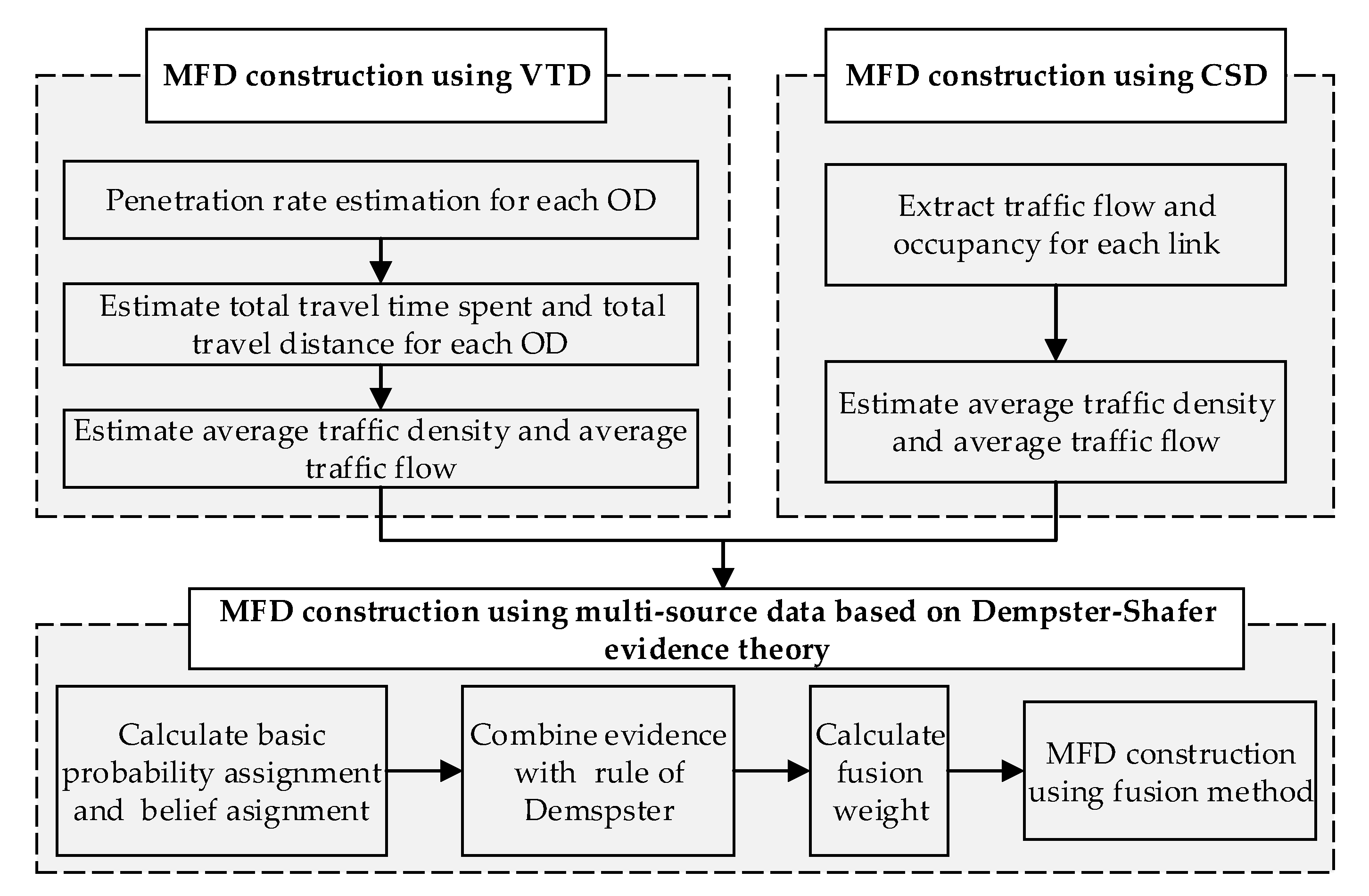
Considering the reliability of different data sources, an MFD construction method is proposed using multi-source data. The framework of the study is shown in Figure 1. The abbreviations in Figure 1 are listed in Appendix (Abbreviations). Firstly, the MFD was constructed based on VTD by estimating the total travel distance (TTD) and total travel time spent (TTS) of all vehicles considering the different penetration rates of probe vehicles in different ODs. Secondly, drawing on existing research, the MFD was constructed based on CSD. Finally, considering the different reliability of different sources of data, the two types of data were fused, and the MFD was constructed based on the DS evidence theory. The contents of each part are described as follows.
- (1)
- MFD construction using VTD
VTD has the advantages of wide spatial coverage and high estimation accuracy of the ATD of the road network, but it also has disadvantages such as a low penetration rate and uneven spatial distribution of probe vehicles. Because of this, firstly, the probe vehicle’s penetration rate of each OD in each period was estimated by the proportion of probe vehicles detected by automatic license plate recognition (ALPR) equipment between each OD. Secondly, the travel time and travel distance of all probe vehicles in each period of each OD in the road network were calculated. Thirdly, the total travel time and total travel distance of all vehicles in each period for the road network were derived from the estimated penetration rate. Finally, the ATD and the ATF of the test site were calculated.
- (2)
- MFD construction using CSD
The traffic flow data for a location of a link are collected by fixed vehicle detectors (such as microwave, video, etc.). The ATF derived from the CSD can accurately reflect the traffic flow of a road networks when the spatial coverage of fixed vehicle detectors is sufficient (such as more than 25% in reference [7]). In view of this, referring to the research of Ortigosa et al. [7], the basic idea of our study is to use link length as weight, and aggregate the links’ traffic density and traffic flow using the CSD to construct an MFD.
- (3)
- MFD construction using multi-source data based on DS evidence theory
Because of the low penetration rate and disequilibrium spatial distribution of probe vehicles, and the insufficient coverage of fixed vehicle detectors in real road networks, the reliability of the two sources of data in the estimation of ATD and ATF is different. Furthermore, there may be inconsistencies if estimating ATD and ATF with different sources of data. Because of this, it is proposed to quantify the fusion weight of different sources of data by their reliability based on the DS evidence theory, and then construct an MFD with the fusion method. The basic idea to determine the fusion weight is introduced as follows: (1) Establish the recognition framework of the DS evidence model based on estimated ATF and ATD for the two sources of data. (2) Quantify the reliability of each source of data for ATF and ATD based on the means and variances of historical data for multiple days; on this basis, calculate the basic probability distribution and basic trust distribution. (3) Synthesize the evidence and calculate the fusion weight of different sources of data based on the Dempster synthesis rule.
3.1. MFD Construction Using VTD
According to Edie’s [21] definition, the parameters of MFD are ATF and ATD, which are linearly related to total travel distance (TTD) and total travel time spent (TTS) of all vehicles, respectively. The specific definitions are shown as Equations (1) and (2),
where q (vehs/h) and k (vehs/km) are ATF and ATD of network traffic, respectively. (veh-km) and (veh-h) are total travel distance and total travel time spent of all vehicles during the research period in the test site, respectively; and (km) is the length of the test site. is the research period, considering the time-varying characteristics of road network traffic; the research period in this paper is 0.25 h.
To estimate the total vehicle travel time and total vehicle travel distance, MFD construction using VTD assumed that the number of probe vehicles is sufficiently large and the penetration rate was homogeneous in all areas of a road network. However, these assumptions are inconsistent with the actual situation. Taking taxis as an example, their distribution often varies greatly in different ODs, and their trips are usually more frequent in the central business district of a city. Given this, we intend to construct an MFD using VTD considering the difference in the penetration rate of probe vehicles between different ODs. The method involves two key issues: first, estimating different OD penetration rates of probe vehicles, and second, estimating the total travel time and total travel distance of all vehicles with the penetration rate.
For the first issue, the penetration rate was estimated based on the vehicle identity and location information collected by probe vehicles, supplemented by traffic flow data collected by ALPR. Then, the penetration rate was estimated as the proportion of probe vehicles detected by ALPR detectors between different ODs. The estimation method [14] is shown in Equation (3):
where and are the first link (link ) and last link (link ) installed with ALPR detectors that the probe vehicles passed by, respectively; is the penetration rate of during period ; and (vehs) and (vehs) denote the count of detected probe vehicles and the count of all detected vehicles from ALPR detectors for during period .
For ODs without ALPR detectors or probe vehicles, the penetration rate was calculated as the proportion of probe vehicles detected by all ALPR detectors in a road network during period . The specific method is shown in Equation (4).
where is the averaged penetration rate for the road network during period , and (vehs) and (vehs) are the counts of probe vehicles and all vehicles detected by ALPR detectors during period , respectively.
With the estimated penetration rate, the total travel time and total travel distance were derived by the sum of the expanded travel time and travel distance of each OD. According to Edie’s definition 20, the travel time and travel distance were converted into the ATD and ATF, respectively. For example, the network traffic flow during period is equal to the number of times of all vehicles running on the road network during period . The specific method is shown in Equations (5) and (6).
where (vehs/h) and (vehs/km) represent the ATF and ATD, respectively, based on VTD during period ; (km) and (h) denote all probe vehicles’ travel distance and travel time, respectively, of in the road network during period ; and and are the count of the first and last links, respectively, installed with ALPR detectors that the probe vehicles passed by during period .
3.2. MFD Construction Using CSD
Generally, detectors are installed in the middle of links of the urban network road in China; therefore, the MFD constructed with CSD is conducted through estimating the ATF and ATD with link length as weight [7]. The specific method is shown in Equations (7) and (8),
where (vehs/h) and (vehs/km) represent the ATF and ATD, respectively, of the road network based on CSD during period ; (vehs/h) and (vehs/km) represent traffic flow and traffic density, respectively, of the -th link installed with fixed vehicle detectors during period ; is the length of the -th link installed with fixed vehicle detector; and is the number of fixed vehicle detectors in road networks.
3.3. A Fusion Method for MFD Construction Using Multi-Source Data
It is theoretically possible to estimate ATF and ATD of road networks based on VTD or CSD. To accurately estimate MFD, some studies [10] used different sources of data to estimate different parameters. However, the assumptions for estimating ATF and ATD with different data sources are different. For ATD estimation, it is generally assumed that the probe vehicles’ amount is sufficient and spatial distribution is uniform. For ATF estimation, it is usually assumed that the traffic flow achieved from detectors is representative. Therefore, there may be inconsistencies in the parameters of MFD using different sources of data to estimate different parameters. Considering the different reliability of different data sources, the basic framework of the fusion method for MFD construction under multi-source data is shown in Equations (9) and (10):
where (vehs/h) and (vehs/km) denote the ATF and ATD with fusion method in, respectively. The meanings of , , and are the same as in Equations (5)–(8). and are the weight of VTD and CSD for traffic flow estimation in, respectively. and are the weight of VTD and CSD for traffic density estimation in, respectively.
The core of the fusion method is to determine the weight of the two types of data. The weights were achieved using the ATF, ATD, and their variance distribution (reliability) for different periods during multiple days based on the DS evidence theory [22]. Taking the estimation of for ATF in as an example, the specific process is described as follows.
First, we establish the recognition framework of the DS evidence inference model based on the two types of data; the specific description is shown as Equation (11):
where and denote the estimated weight of CSD and VTD for ATF in , respectively.
Since and come from different sources of data, they can be considered mutually exclusive. Thus, the power set composed of all elements in is shown in Equation (12):
where is the empty set; is norm of , namely, the non-zero element of ; and are non-empty sub-collections of , (vehs/h), and (vehs/h), respectively. The first two denote the decision of ATF based on CSD and VTD, while is an uncertain decision, which means it cannot determine the decision between and .
Secondly, DS evidence theory involves two important concepts: basic trust distribution (also known as evidence function) and the Dempster evidence synthesis rule. The basic trust distribution is an indicator to quantify the support degree for a certain decision (namely, the evidence of each decision). The evidence synthesis rule is a comprehensive analysis rule of pieces of evidence corresponding to each decision. Let : , meaning that the basic trust distribution is a mapping , which needs to satisfy the requirements described in Equation (13):
where is the -th evidence provided by the -th type of data, and is the -th decision. The meanings of and are the same as in Equation (12). represents the degree of support for the decision provided by the -th type of data evidence, which is equal to the basic trust distribution of decision . The basic trust value of the empty set is 0, and the sum of the trust of the other subset is equal to 1.
The basic trust distribution is determined by the basic probability distribution function of the decision under each type of data; the specific method is shown in Equation (14).
where the meaning of is the same as in Equation (13), and is the basic probability distribution function of decision under different types of data.
Assuming that satisfies , where and represent the mean and variance (i = 1, 2) of ATF during period for the historical data of the -th type of data, can be calculated according to Equation (15) [22]:
where are the integral intervals to calculate with given . Moreover, ,, and represent the occurrence probability of decisions , , and , respectively, under the evidence provided by different types of data.
Based on the basic trust assignment of the decision , the evidence synthesis is conducted with the basic probability assignments of multiple types of evidence using the Dempster evidence synthesis rule [22]. The specific method is shown in Equation (16):
where , is synthetic trust distribution, and is the decision provided by the evidence of the -th type of data. is the conflict coefficient between evidence provided by different types of data, calculated as ; the closer is to 0, the greater the degree of conflict between the evidence provided by different data sources is, and when , the sum under the Dempster evidence synthesis rule does not exist.
Finally, the fusion weight is determined by the synthetic trust distribution; the method to calculate the weight for is shown in Equation (17):
where, the meaning of is the same as in Equation (9), and , and represent the synthetic trust distribution of each decision under the evidence provided by each type of data. The abbreviations and variables used in the paper are listed in the Abbreviations.
4. Case Study
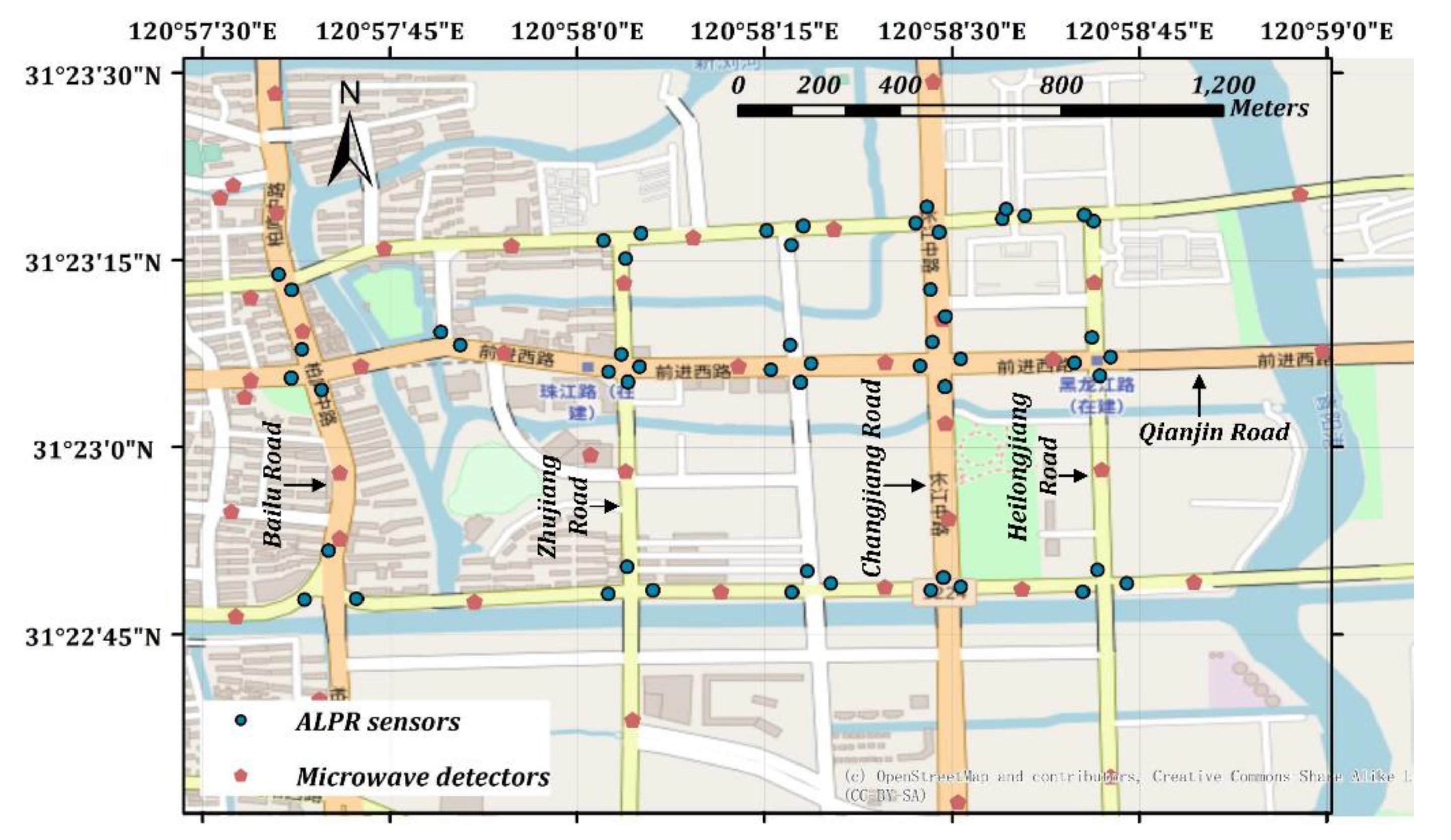
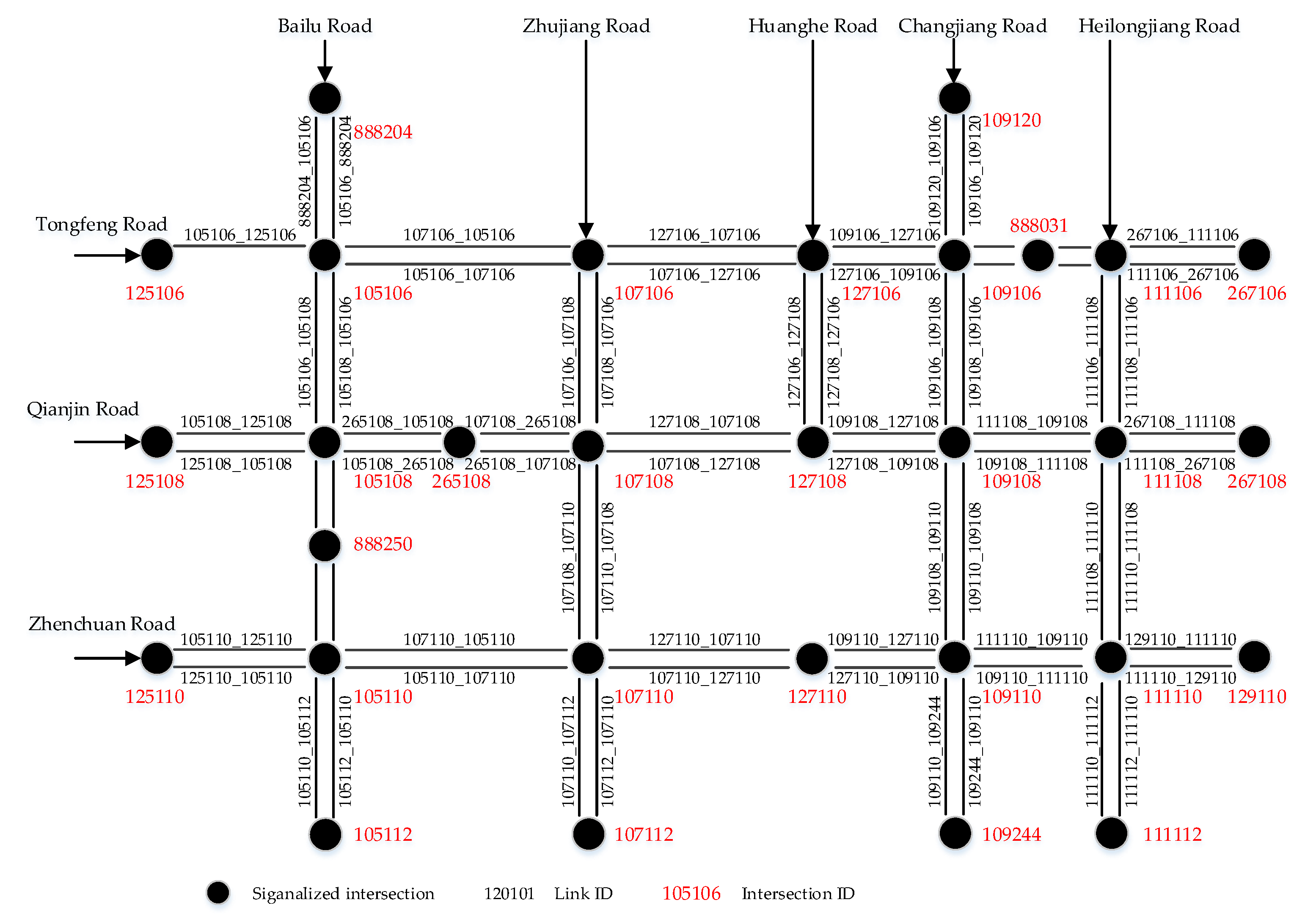
The road network in the central urban area of Kunshan was selected as the test site. The test site consists of 71 links and 18 intersections, including links that are prone to traffic congestion, such as Qianjin Road, Bailu Road, and Zhenchuan Road. The data were provided by a real-time monitoring system of urban road traffic conditions in Kunshan city. The system integrates data collected by microwave vehicle detectors, automatic license plate recognition (ALPR) equipment, GPS-equipped taxis, etc. There are 54 sets of ALPR equipment and 33 sets of microwave vehicle detectors. Figure 2 shows the distribution of various devices, and Figure 3 shows the abstract topology of the test site. The data used in our study were from 3 January 2018 to 20 January 2018.
4.1. Data Preprocessing for VTD
The VTD (from the taxis in Kunshan city) consists of the vehicle license plate, time, longitude, latitude, vehicle speed, driving direction, etc. The data are updated every 20 s. An example of the data is shown in Table 2. After map-matching, there are about 1500 taxis in the study area every day.
The preprocessing for VTD mainly includes the followings steps [23,24]: (1) Given the error of the satellite’s positioning, the VTD is matched with links’ positions. (2) Considering that taxis may stop for a long time to pick up and drop off, or wait for customers, these trajectory points with long-term parking were marked as abnormal data. (3) Considering the spatio-temporal continuity of trajectory data, the discontinuous links between two adjacent points were marked as abnormal data, and abnormal changes in the distance between the downstream intersection and two adjacent points in the same link were also marked as abnormal data. (4) Based on the valid trajectory data, each OD’s count of taxis and each OD’s taxi travel time and travel distance were calculated.
4.2. The Data Preprocessing for ALPR Data
Kunshan city’s ALPR data were collected when vehicles passed stop lines at road intersections. The data consist of ALPR equipment’s ID, date, vehicle license plates, passing time, passing lane, etc. (an example is shown in Table 3). Among them, the equipment’s ID is the unique identification of each device, the passing time represents the time when the vehicle passes the stop line of the entrance, and the passing lane represents the lane where the vehicle was located. Affected by equipment failure, data transmission failure, image recognition quality, etc., there may be problems such as unrecognized vehicle number plates and duplicate records. In view of this, the ALPR data were preprocessed, including time regularization, removal of duplicate records, removal of unrecognized data [25,26], etc. It should be noted that the ALPR data are only used to extract the traffic flow of link; the vehicle trajectory reconstruction is not considered to construct an MFD. The main reasons include three aspects: (1) limited by the cost, ALPR equipment’s coverage is limited, and the vehicle trajectory obtained after vehicle license plate matching is fragmented in time and space; (2) the inflow and outflow of vehicles between the ALPR equipment is serious; and (3) the ALPR equipment in our study only covers the straight and left-turn lane groups.
4.3. The Preprocessing for Microwave Detector Data
Kunshan city’s microwave vehicle detectors are mostly installed in the middle of the links. The traffic flow data of a lane were collected every 30 s. The data consist of the equipment ID, lane ID, date, time, flow, speed, time occupancy, etc. (see Table 4 for a sample of the data). In the table, the device ID is the unique identification of each microwave detector, the flow rate is the number of vehicles passing through a detector in a lane within 30 s, the speed is the average speed of all vehicles passing a detector in a lane within 30 s, and the time occupancy rate is time occupancy of a lane over 30 s.
Due to the equipment transmission failure and equipment failure, some microwave data are abnormal. In view of this, the microwave detector data are preprocessed. The preprocessing consists of a data validity test and data aggregation. The data validity test was conducted referring to Ref. [27], aiming to identify abnormal data. Data aggregation includes two aspects: temporal aggregation and spatial aggregation of traffic flow data. Temporal aggregation refers to the aggregation of traffic flow data from the original 30 s interval to the period required for the study, and spatial aggregation refers to aggregate traffic flow of lanes to links and aggregate traffic flow of sections to links [27]. The period for MFD construction is 15 min in our study.
5. Results
This section consists of three parts: a case study, results, and the evaluation. The specific contents are introduced as follows.
5.1. Results of Key Parameters of MFD Construction Using Multi-Source Data
The key parameters of the proposed method for MFD construction include TTS and TTD of probe vehicles, probe vehicles’ penetration rate, and ATF and ATD of the road network of CSD.
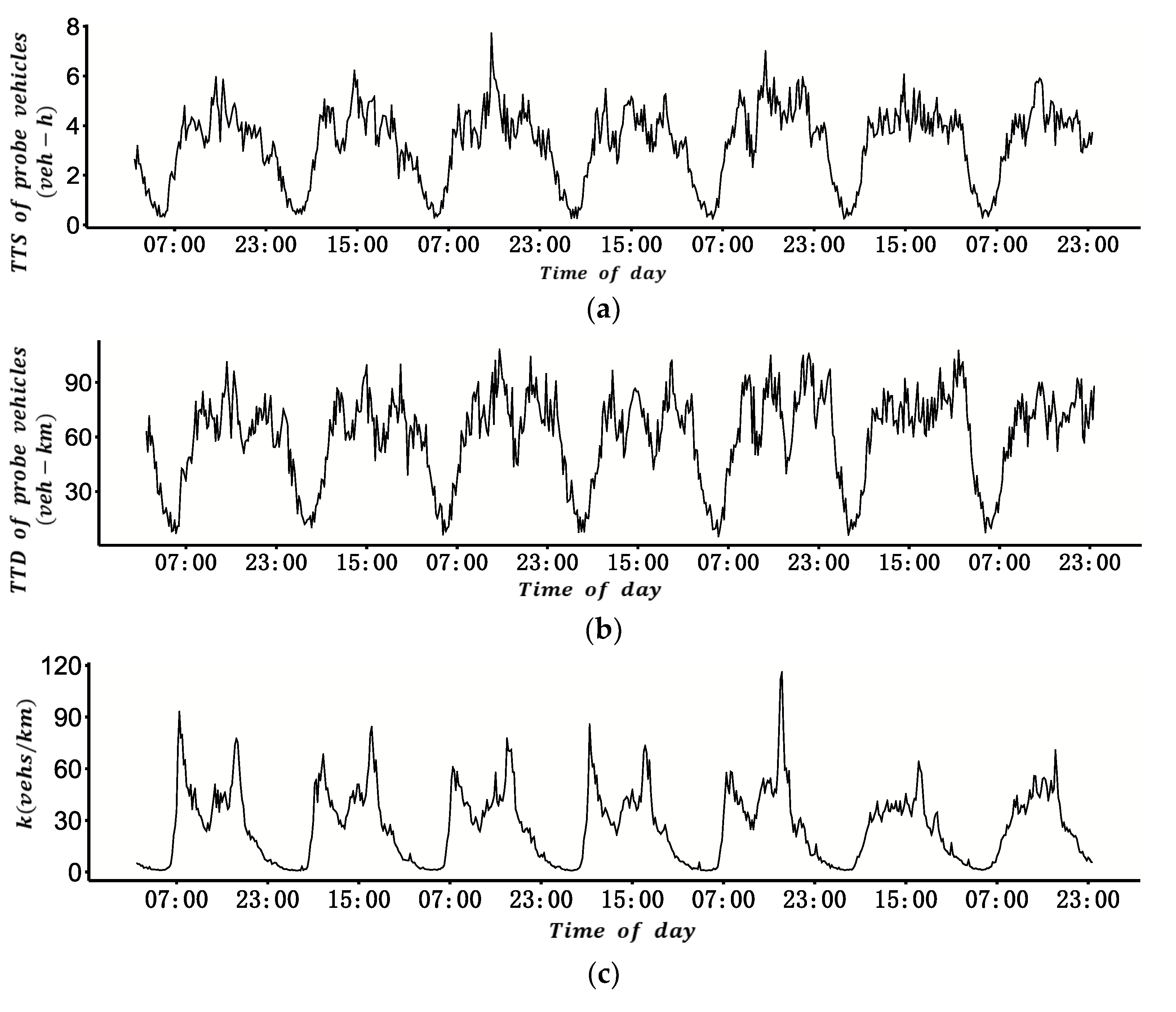
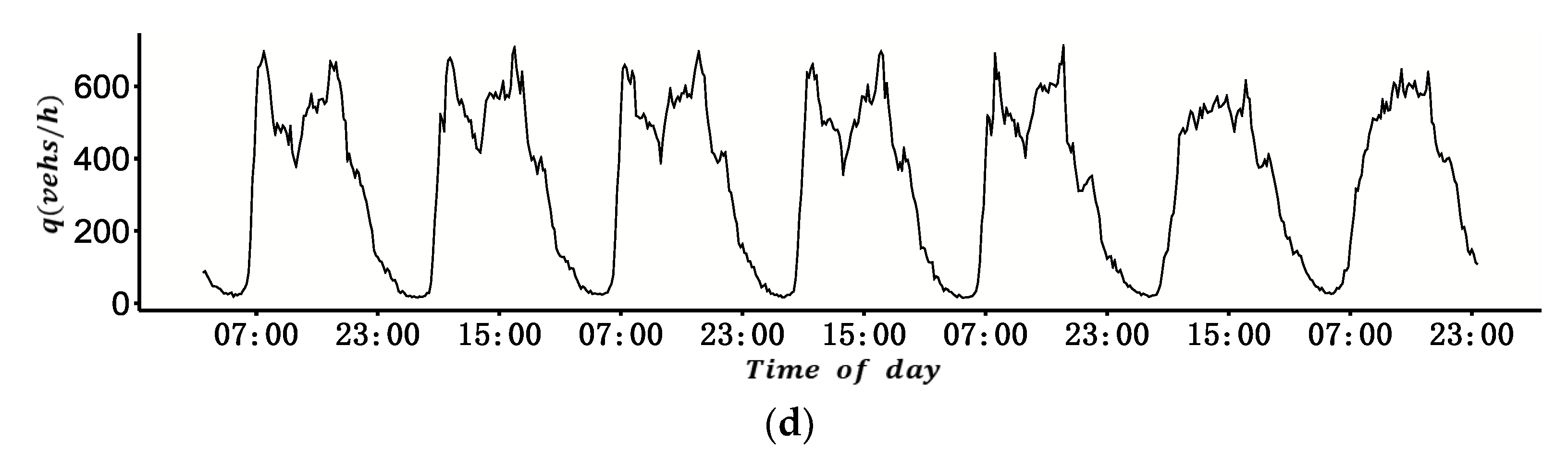
The estimation of TTS and TTD of probe vehicles directly affects the accuracy of the MFD. Figure 4a,b shows the travel time and total travel distance of all probe vehicles in a 15 min period from 8 to 14 January 2018 without expansion. January 8 to 12 are weekdays, and 13 and 14 January are weekends.
Figure 4a,b shows that the changing trend of all probe vehicles’ travel time and travel distance every 15 min for the test site during the peak period is similar. The variation in the two parameters between different periods is larger on weekdays, while the changes on weekends are relatively minor. The main reason is that there are many commuting trips at the test site on weekdays, and the travel time and travel distance of all probe vehicles are quite different during peak and off-peak periods. However, on weekends, there are fewer commuting vehicles and there are no obvious morning and evening peaks. The results are consistent with the actual traffic. Figure 4c,d shows the time series of ATF and ATD based on the CSD of the test site from 8 to 14 January 2018. It shows that the ATF and ATD of the test site on weekdays have obvious morning and evening peaks, and are significantly larger than those on weekends. Considering that there are many commuting trips on weekdays, the results of the case study are consistent with the actual traffic.
Table 5 shows the penetration rate of probe vehicles in some ODs from 7:00 a.m. to 07:15 a.m. from 3 January 2018 to 20 January 2018. The link IDs of origins and destinations in the table are the same as those in the road network topology in Figure 3. It shows that the penetration rate of probe vehicles in different ODs is significantly different, which reflects the uneven spatial distribution of probe vehicles.
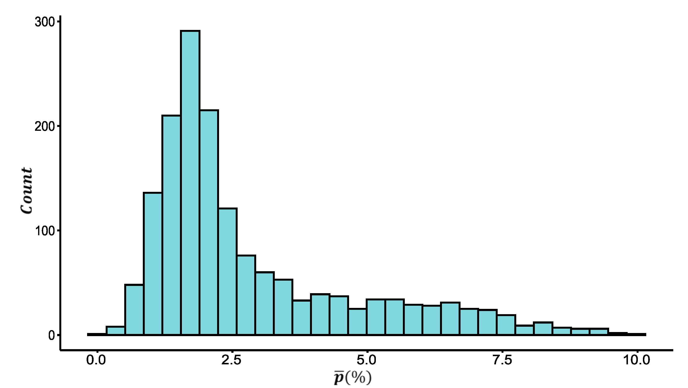
Figure 5 shows the statistical distribution of the probe vehicles’ penetration rate at each period from 3 January to 20 January 2018. The horizontal axis represents the average penetration rate of the test site in each period, and the vertical axis represents the period’s frequency corresponding to specific penetration rate. It shows that the median penetration rate in the test site is about 2%. Ref. [28] estimated the penetration rate of probe vehicles in the central urban area of Kunshan to be 1.8% during off-peak periods and about 1.5% during the peak period. Since the central area of Kunshan where congestion is frequently presented is selected in our study, more probe vehicles’ trips are presented, so the penetration rate is slightly higher. The estimated results for the penetration rate in our study are consistent with Ref. [28].
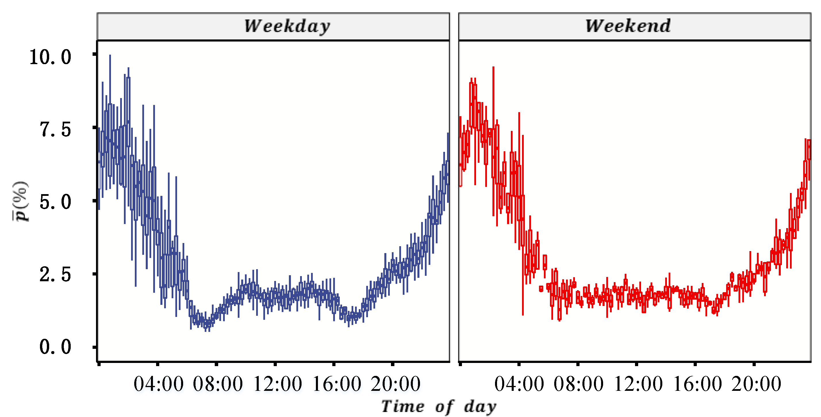
Figure 6 shows the boxplot of each period’s penetration rate for weekdays and weekends within 18 days. It can be seen from the figure that the penetration rates at certain periods have obvious differences. Specifically, the penetration rate is relatively high and has a large range from 8:00 p.m. to 6:00 a.m. the next day, while it is relatively low and has a small range from 6:00 a.m. to 8:00 p.m. Judging from the changing trend between weekdays and weekends, the penetration rate also seems different at certain periods. Specifically, the penetration rate has relatively obvious peaks on weekdays. Considering that taxis (probe vehicles) travel frequently at night compared to social vehicles, and that social vehicles generally present at other periods, the penetration rate of probe vehicles is higher at night. In addition, since social vehicle travel at night is lesser and more unstable, its impact on the penetration rate of probe vehicles is greater. The results of the case study are consistent with the actual traffic.
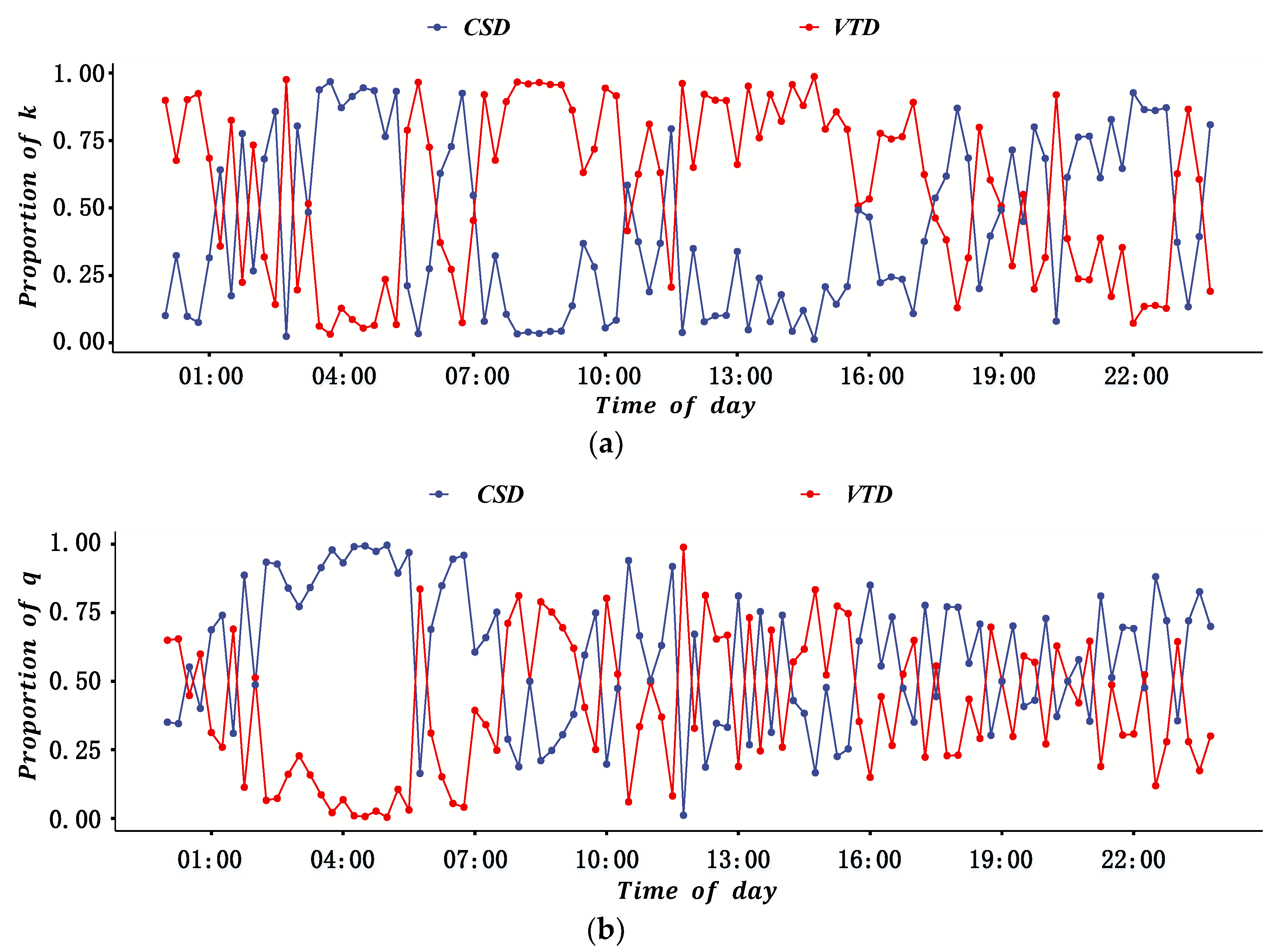
Based on the estimated key parameters, MFD construction under multi-source data was conducted. Considering the stability of fusion weight estimation under different sources of data, the dynamic fusion weights of different periods were estimated. The results of dynamic fusion weights for weekdays are shown in Figure 7.
In Figure 7, the blue and red dots represent the fusion weights of each parameter in each period under CSD and VTD, respectively. It reveals that the fusion weights of the MFD parameters in different periods are significantly different. For the fusion weight estimation of ATD of the test site (Figure 3, Figure 4, Figure 5, Figure 6 and Figure 7a), the weight of the VTD is greater in most periods, and the overall weight is 0.637 on weekdays. For the fusion weight estimation of ATF of the test site (Figure 3, Figure 4, Figure 5, Figure 6 and Figure 7b), the weight of the CSD is slightly larger in most periods (the weight of VTD in some periods is larger; the reason may be that the fixed vehicle detector has detected the queue at these periods, and fixed vehicle data reliability is lower compared to VTD), and the overall weight is 0.551 on weekdays. The estimation of ATD is more accurate using VTD compared with CSD because the spatial coverage of the probe vehicle data is wider, and the estimation of traffic density is easily affected by the location of fixed detectors. However, the sample size is not large enough and the penetration rate is not sufficient; therefore, the estimation for ATF is more accurate using CSD compared with VTD. The results of the case study are consistent with the qualitative analysis results of the two types of data.
5.2. Results of MFD Construction Based on Multi-Source Data
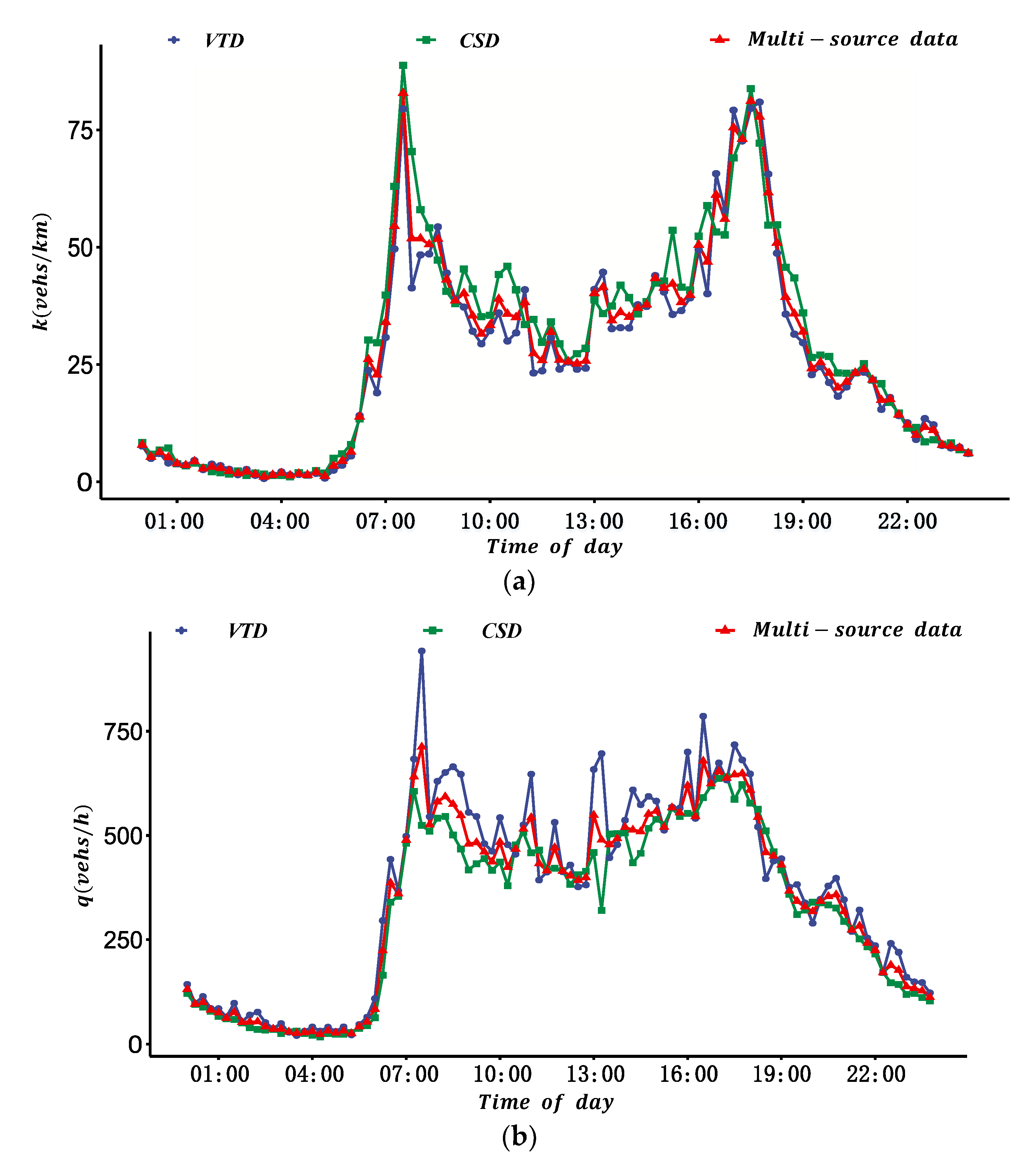
In this section, we focus on the analysis of the constructed MFDs. Figure 8 shows the ATF and the ATD of the test site estimated by VTD, CSD, and multi-source data. Taking the MFD on 4 January 2018 as an example, Figure 8a,b shows the estimated ATD and ATF under different sources of data for the test site. In the figure, the blue round scatter points, green square scatter points, and red triangle scatter points represent the estimated ATD and ATF based on VTD, CSD, and multi-source data in each period, respectively.
Figure 8 shows that the constructed MFDs under different sources of data are consistent, and the change trends of ATD and ATF of the test site under the three types of data are similar. The ATD of the test site under different data sources is similar in most periods. However, the estimated ATF of the test site based on VTD is significantly higher in some periods (such as morning peak and evening peak).
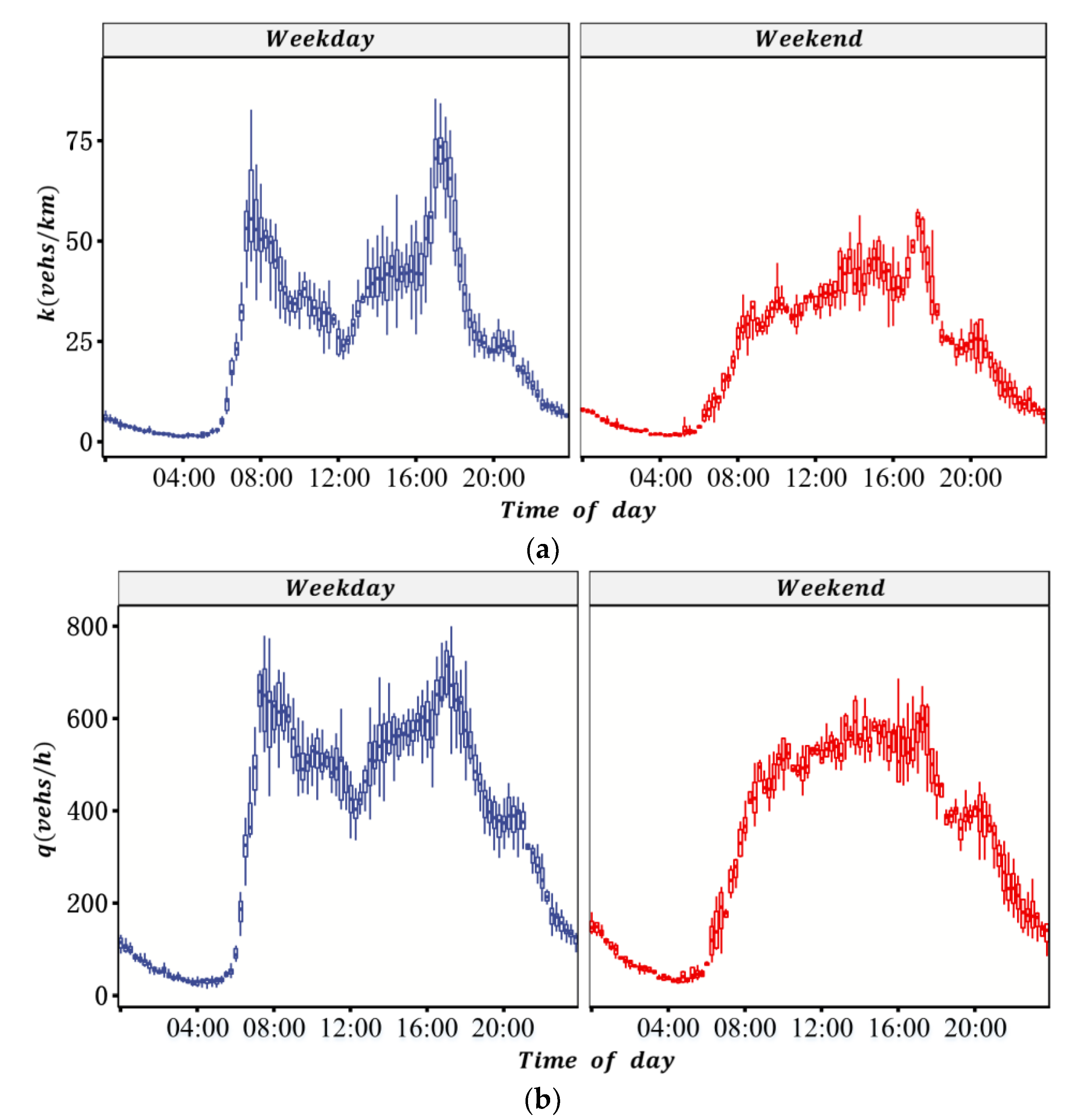
Figure 9 is the boxplot of the ATD and ATF of the test site for each period on weekdays and weekends within 18 days. It is shown that the median ATD and median ATF are significantly different between weekdays and weekends. The ATD of the test site during peak hours on weekdays can reach 75 vehicles/km, and the ATF is about 700 vehicles/h; the ATD during peak hours on weekends is about 50 vehicles/km, and the ATF is about 600 vehicles/h. The distance between the upper and lower edges of the ATF and ATD in the boxplot at each period on weekends is significantly smaller than that in the same period on weekdays, and the ATD and ATF of the test site on weekends have no obvious morning and evening peaks.
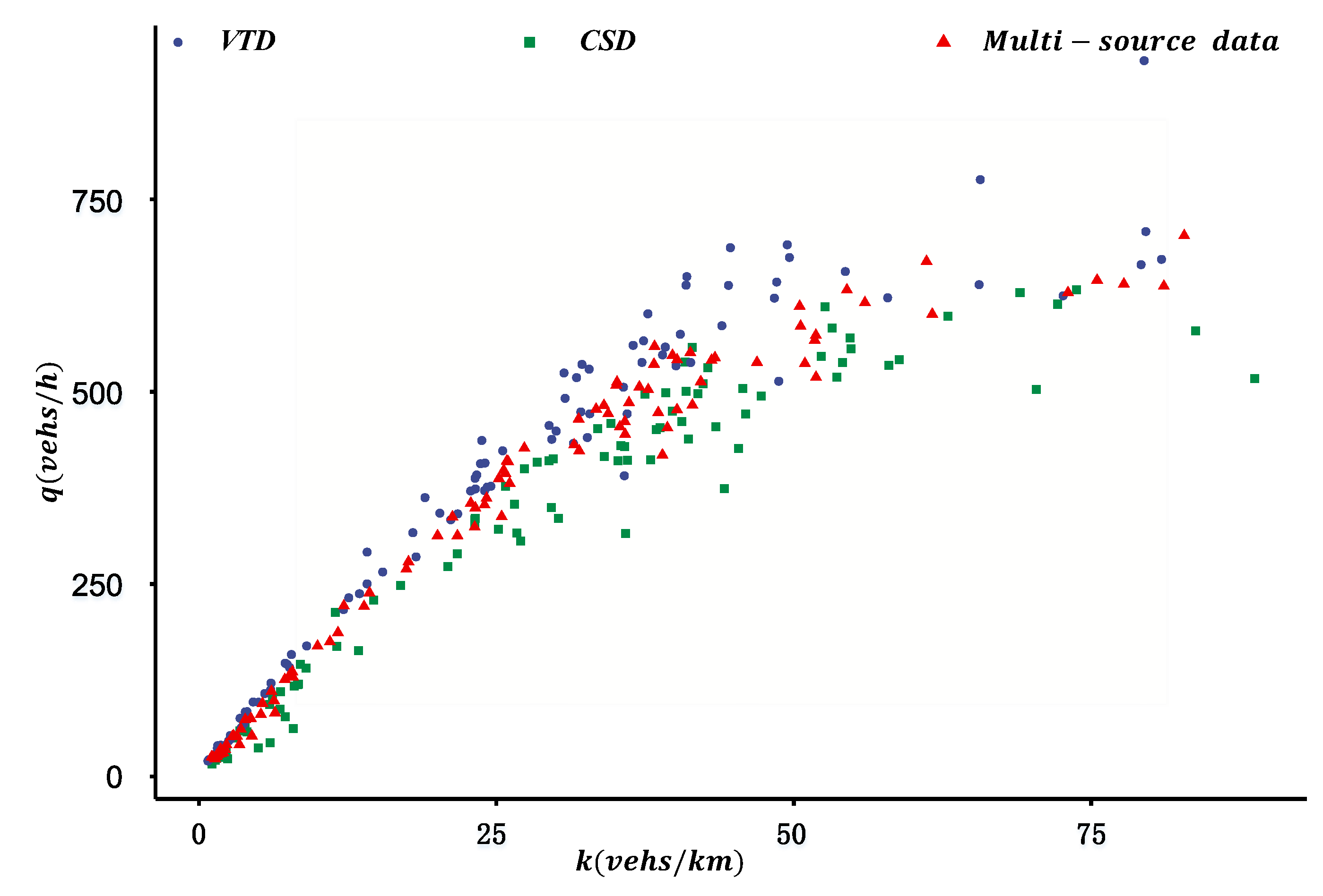
Figure 10 shows the scatter plots of the constructed MFDs using different types of data. In the figure, the blue circles, green squares, and red triangles represent the constructed MFDs based on the VTD, CSD, and multi-source data for each period, respectively. It can be seen from the figure that there are many abnormal points in the MFD under the VTD, and the ATF of the test site in some periods is significantly higher. It is concluded that the ATF estimation using VTD is less stable. The estimation of ATF based on the CSD has small fluctuations, but the estimation of the ATD has large fluctuations. The stability of the estimation of the ATD and the ATF under the multi-source data is between VTD and CSD.
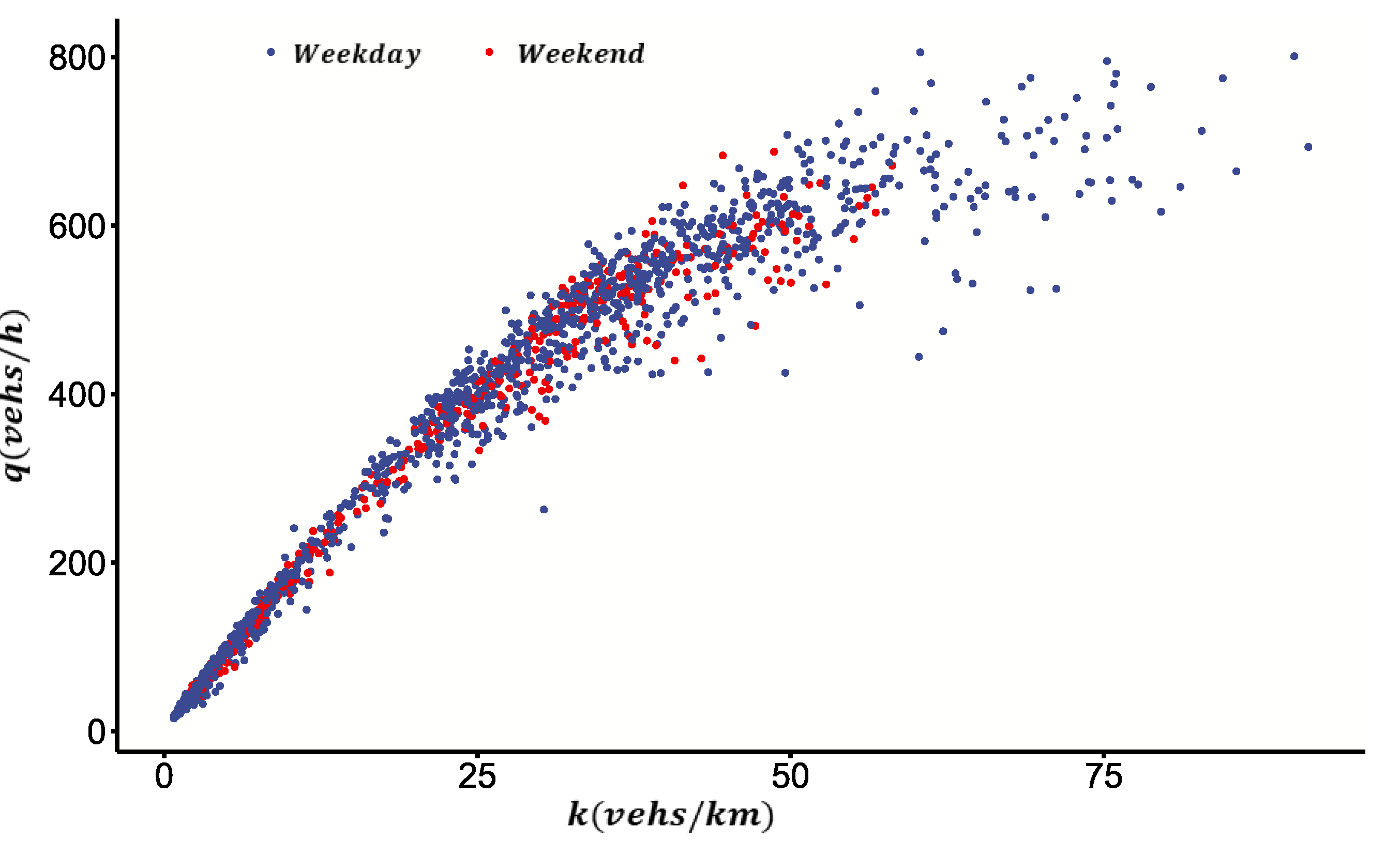
Figure 11 shows the scatter plot of the constructed MFDs of weekdays and weekends under multi-source data. In the figure, the horizontal axis and the vertical axis represent the ATD and ATF of the test site (blue dots for weekdays, red dots for weekends), respectively. It is shown that there is a significant difference in the MFD between weekdays and weekends. The range of ATD and ATF on weekdays is significantly wider. Most of the points whose ATD is greater than 60 vehicles/km or traffic flow is greater than 600 vehicles/hour come from weekdays. Given that there is indeed a large number of commuting trips at the test site on weekdays, the results of the case study are consistent with the actual traffic.
The results in Figure 11 reveal that the traffic state of the test site is not over-saturated (with the increasing ATD, ATF shows a downward trend), which may be related to the heterogeneity of the traffic flow of links in the test site. The heterogeneity is general in actual urban traffic networks. Moreover, the evaluation of the proposed method is difficult to realize with real data. Therefore, it is intended to analyze MFD with an over-saturated state and evaluate the performance of the proposed method using simulated data.
5.3. The Evaluation of Constructed MFD’s Accuracy Based on Traffic Simulation
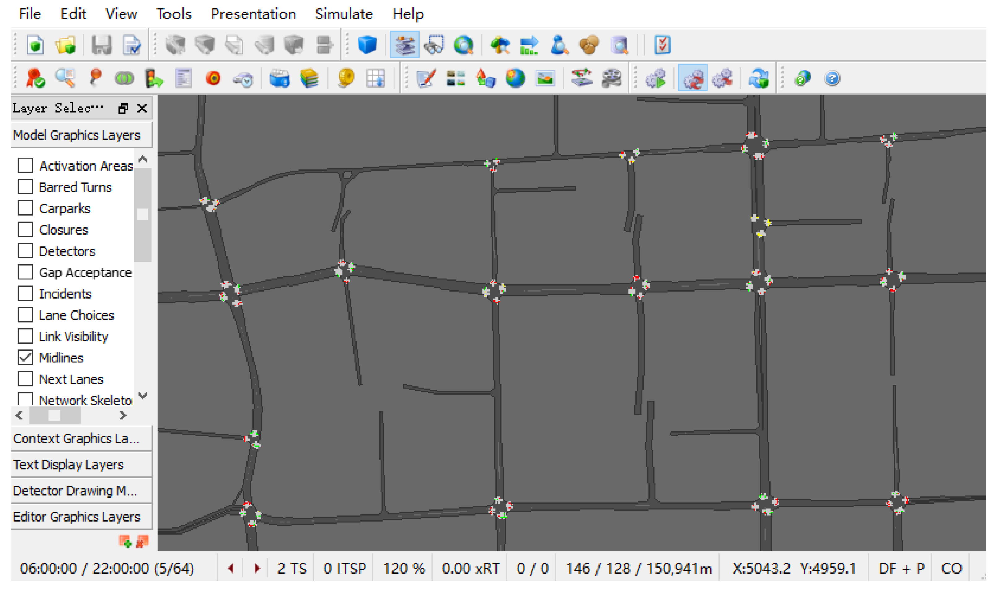
Because of the difficulty of evaluating the accuracy of the proposed method based on real traffic data, the actual traffic of the test site was simulated based on Q-PARAMICS (Quadtone Parallel Microscopic Simulator), and the VTD, CSD, and ALPR data were output. On this basis, the MFD under different sources of data is constructed based on the simulation data, and the accuracy of the proposed method is evaluated. Also based on the test site, the simulated road network is shown in Figure 12 (considering the comparability of the MFD constructed from the actual data and the simulated data, the simulated road network is consistent with the actual one). Based on the traffic flow data of links and intersections that can be observed in 15 min, this paper refers to the method of Ref. [29] to calibrate parameters such as traffic demand and the link’s traffic capacity for traffic simulation. The start time of the simulation is 06:00:00, and the duration is 16 h.
To evaluate the accuracy of the MFD construction method, the CSD for every 5 min and all vehicles’ trajectory data with 0.5 s’ updated frequency were extracted based on traffic simulation. The examples of extracted data are shown in Table 6 and Table 7 (the vehicle position coordinates in the VTD are from the traffic simulation software). It is worth noting that the actual simulated road network is larger than that shown in Figure 12, and the vehicles’ ODs are not limited to the selected area.
To evaluate the accuracy of the proposed method, MFDs of 10 scenarios were constructed with the penetration rate of probe vehicles (5% to 10%) and the coverage rate of fixed vehicle detectors (15% to 90%) and then compared with the MFD under all vehicles’ data. Referring to the research of Saffari et al. [30], the root mean square error between partial samples and full samples was selected as the accuracy evaluation index, and the calculation method is shown in Equation (18):
where is the root mean square error for ATF and ATD of the test site; and (vehs/h) denote the ATF derived from simulated full-sample data and simulated multi-source data during period , respectively; and (vehs/km) are ATD derived from simulated full-sample data and simulated multi-source data during period , respectively; is the count of periods; Q (vehs/h) is the network traffic capacity; (vehs/km) is the maximum ATD, referring to the research of Saffari et al. [30]; and is approximated as the mean of the first three maximum ATDs.
Table 8 shows the errors of the constructed MFDs with different data sources in each scenario. The improvement in the table refers to the difference between the errors of the current method and the proposed method (MFD fusion construction), and I, II, III, and IV represent MFD construction using simulated CSD, simulated VTD, different sources of data, and simulated multi-source data, respectively. It can be seen from the table that the error of the proposed method is smaller (with a minimum of 7.7%) than that of other methods. For the same scenario, compared with MFD construction using simulated CSD, the error of the constructed MFD is reduced by 11% based on the fusion method. Furthermore, for the same scenario, compared with MFD construction using simulated VTD, the error of the constructed MFD is reduced by 22.3% based on the fusion method. Compared with MFD construction through estimating different parameters separately, the error of the constructed MFD is reduced by 8.1% based on the fusion method. The errors of Scenario 4 and Scenario 8 are as high as 39.5% and 48.5% for simulated VTD, respectively, which reflects the instability of MFD construction based on simulated VTD.
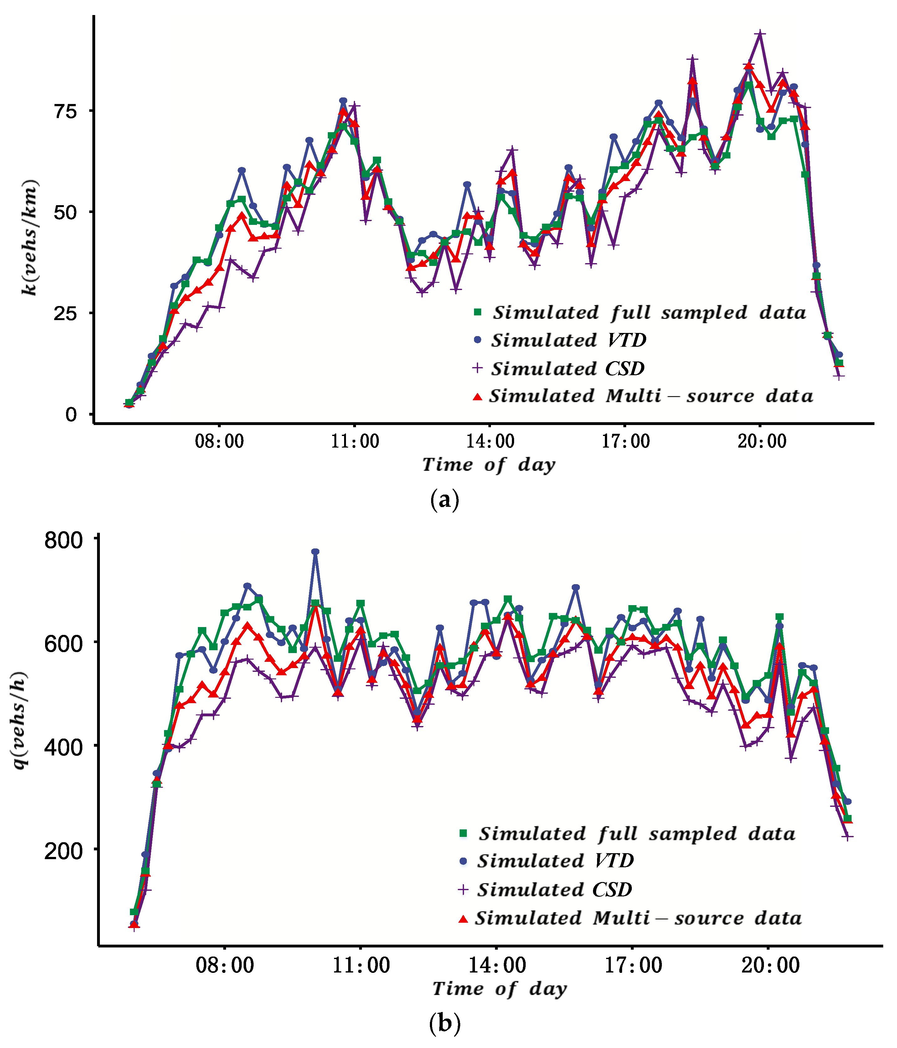
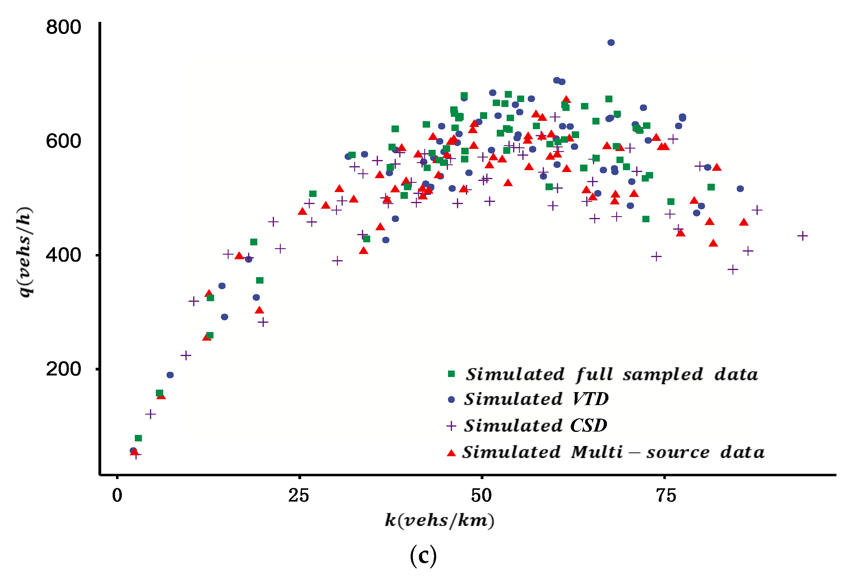
Taking the scenario in which probe vehicles’ penetration rate is 10% and fixed vehicle detectors’ coverage rate is 15% as an example, Figure 13 shows the results of a constructed MFD based on different sources of data. In the figure, the scatter points with blue circles, green squares, purple plus signs, and red triangles represent the estimated traffic density and traffic flow derived from the simulated VTD, simulated full sample data, simulated CSD, and simulated multi-source data for each period, respectively. It can be seen from the figure that the MFD under various data sources is generally consistent. The changing trends of MFD under the three sources of data in different periods are the same, and the values are similar, which confirms the rationality of the proposed method.
The results in Figure 13 reveal that the accuracy of estimated ATF is higher based on simulated CSD compared with that derived from simulated VTD, but the accuracy of estimated ATD is not accurate enough based on simulated CSD. The results also reveal that the MFD under multi-source data integrates the advantages of the two types of data, and the accuracies of estimated ATF and ATD are between those derived from the other two types of data. In addition, like the results of real data, the estimated ATF under the simulated VTD is significantly higher in some periods, and the error is large. In general, the accuracy and stability of MFD construction by the fusion method under multi-source data are higher.
6. Conclusions and Discussion
In this study, we proposed an MFD construction method based on multi-source data, as follows: First, estimate the travel time and travel distance of probe vehicles of each OD, and estimate the probe vehicles’ penetration rate of each OD with the percentage of probe vehicles collected by fixed vehicle detectors. On this basis, the vehicles’ travel time and travel distance are expanded, and then the average traffic density and average traffic flow are estimated. Secondly, the traffic density and traffic flow of each link are collected, and the MFD under cross-sectional traffic flow data is constructed. Finally, considering the historical distribution characteristics of the average traffic density and average traffic flow in each period for different data sources, the reliability of each data source is quantified. On this basis, the MFD under multi-source data is constructed based on DS evidence theory.
Taking the congested area of Kunshan city, Jiangsu province, as the test site, the results for actual and simulated scenarios were analyzed, and the performance of the proposed method was evaluated. The results of the case study show that the changing trends of MFD in different periods under the three data sources are the same, and the values are similar, confirming the reliability of the proposed method. The results also show the high accuracy (with a minimum error of 7.7%) of the constructed MFD under multi-source data. For the same scenario, the MFD construction error of the fusion method has a maximum reduction of 11% compared with that only using cross-sectional traffic flow data, a maximum reduction of 22.3% compared with that only using vehicle trajectory data, and a maximum reduction of 8.1% compared with that based on estimates of different parameters using different data sources. In summary, the proposed method can significantly improve the accuracy of constructed MFDs by combining the advantages of the two types of data. It provides potential to support the evaluation of traffic operation and the optimization of the signal control schemes for urban traffic networks. However, due to the limitations of data availability, the accuracy of the proposed method cannot be evaluated in cities with severe congestion (such as Beijing), whose descending part of MFD would present. In the future, the impact factors that affect the accuracy of constructed MFDs will be investigated through comparative analysis. Additionally, more field validation works are needed to validate the effectiveness of the proposed method.
Author Contributions
This paper was written by R.H. in collaboration with all co-authors. Data were collected by H.L. The results were analyzed by R.H. and H.L. The research and key elements of the models were reviewed by B.W., Z.L. and J.X. The writing work for corresponding parts was completed by R.H., H.L. and C.A. All authors have read and agreed to the published version of the manuscript.
Funding
This research was funded by the National Natural Science Foundation of China, grant number 71971060.
Data Availability Statement
The data presented in this study are available on request from the first author. The data are not publicly available due to licensing restrictions from data providers.
Conflicts of Interest
The authors declare no conflict of interest.
Abbreviations
| ALPR data | Automatic license plate recognition data |
| ATD | Average traffic density of road network |
| ATF | Average traffic flow of road network |
| CSD | Cross-sectional data of traffic flow |
| DS evidence | Dempster–Shafer evidence theory |
| GPS | Global positioning system |
| MFD | Macroscopic Fundamental Diagram |
| OD | Origins and destinations |
| Q-PARAMICS | Quadtone Parallel Microscopic Simulator |
| TTS | Total travel time spent |
| TTD | Total travel distance |
| VTD | Vehicle trajectory data |
| The count of detected probe vehicles from ALPR detectors for during period | |
| The count of probe vehicles detected by ALPR detectors during period (vehs) | |
| ATD derived from simulated full-sample data and simulated multi-source data during period | |
| The maximum ATD (vehs/km) | |
| The length of road network(km) | |
| The count of all detected vehicles from ALPR detectors for during period | |
| The count of all vehicles detected by ALPR detectors during period (vehs) | |
| The length of -th link installed with fixed vehicle detector | |
| The count of the first links and last links installed with ALPR detectors that the probe vehicles passed by during period | |
| The first and last link installed with ALPR detectors that the probe vehicles passed by | |
| The penetration rate of during period | |
| The averaged penetration rate for road network during period | |
| The basic probability distribution of the decision under each type of data | |
| Average traffic flow (vehs/h), average traffic density (vehs/km) | |
| The average traffic flow and traffic density based on vehicle trajectory data during period | |
| The average traffic flow and average traffic density based on cross-sectional data during period | |
| The traffic flow and traffic density of the -th link installed with fixed vehicle detector during period | |
| The average traffic flow and traffic density with fusion method | |
| The ATF derived from simulated full-sample data and simulated multi-source data during period | |
| The network traffic capacity (vehs/h) | |
| The root mean square error for ATF and ATD of the test site | |
| The degree of support for the decision provided by the -th type of data evidence | |
| Probe vehicles’ travel distance and travel time of in road network during period | |
| The number of fixed vehicle detectors | |
| Research period | |
| The weight of VTD and CSD for traffic flow estimation during period | |
| The weight of VTD and CSD for traffic density estimation during period | |
| The recognition framework of DS evidence inference model during period | |
| The decision of ATF based on CSD and VTD | |
| Uncertain decision in DS evidence model | |
| The mean and variance of ATF during period for the historical data of the -th type of data | |
| The conflict coefficient between evidence provided by different types of data |
References
- Geroliminis, N.; Daganzo, C.F. Existence of urban-scale macroscopic fundamental diagrams: Some experimental findings. Transp. Res. Part B Methodol. 2008, 42, 759–770. [Google Scholar] [CrossRef] [Green Version]
- Zheng, L.; Wu, B. A Reinforcement Learning Based Traffic Control Strategy in a Macroscopic Fundamental Diagram Region. J. Adv. Transp. 2022, 2022, 1–12. [Google Scholar] [CrossRef]
- Zhao, C.; Liao, F.; Li, X.; Du, Y. Macroscopic modeling and dynamic control of on-street cruising-for-parking of autonomous vehicles in a multi-region urban road network. Transp. Res. Part C Emerg. Technol. 2021, 128, 103176. [Google Scholar] [CrossRef]
- Barmpounakis, E.; Montesinos-Ferrer, M.; Gonzales, E.J.; Geroliminis, N. Empirical investigation of the emission-macroscopic fundamental diagram. Transp. Res. Part D Transp. Environ. 2021, 101, 103090. [Google Scholar] [CrossRef]
- Ambühl, L.; Loder, A.; Becker, H.; Menendez, M.; Axhausen, K.V. Evaluating London’s congestion charge: An approach using the macroscopic fundamental diagram. In Proceedings of the 7th Transport Research Arena (TRA 2018), IVT, ETH Zurich, Vienna, Austria, 16–19 April 2018. [Google Scholar]
- Zhang, Y.; Su, R.; Zhang, Y. A macroscopic propagation model for bidirectional pedestrian flows on signalized crosswalks. In Proceedings of the 2017 IEEE 56th Annual Conference on Decision and Control (CDC), Melbourne, VIC, Australia, 12–15 December 2017; pp. 6289–6294. [Google Scholar]
- Ortigosa, J.; Menendez, M.; Tapia, H. Study on the number and location of measurement points for an MFD perimeter control scheme: A case study of Zurich. EURO J. Transp. Logist. 2014, 3, 245–266. [Google Scholar] [CrossRef]
- Buisson, C.; Ladier, C. Exploring the Impact of Homogeneity of Traffic Measurements on the Existence of Macroscopic Fundamental Diagrams. Transp. Res. Rec. J. Transp. Res. Board 2009, 2124, 127–136. [Google Scholar] [CrossRef]
- Courbon, T.; Leclercq, L. Cross-comparison of Macroscopic Fundamental Diagram Estimation Methods. Proc. Soc. Behav. Sci. 2011, 20, 417–426. [Google Scholar] [CrossRef] [Green Version]
- Leclercq, L.; Chiabaut, N.; Trinquier, B. Macroscopic Fundamental Diagrams: A cross-comparison of estimation methods. Transp. Res. Part B Methodol. 2014, 62, 1–12. [Google Scholar] [CrossRef]
- Tilg, G.; Amini, S.; Busch, F. Evaluation of analytical approximation methods for the macroscopic fundamental diagram. Transp. Res. Part C Emerg. Technol. 2020, 114, 1–19. [Google Scholar] [CrossRef]
- Nagle, A.S.; Gayah, V.V. Accuracy of Networkwide Traffic States Estimated from Mobile Probe Data. Transp. Res. Rec. J. Transp. Res. Board 2014, 2421, 1–11. [Google Scholar] [CrossRef]
- Ambühl, L.; Menendez, M. Data fusion algorithm for macroscopic fundamental diagram estimation. Transp. Res. Part C Emerg. Technol. 2016, 71, 184–197. [Google Scholar] [CrossRef]
- Du, J.; Rakha, H.; Gayah, V.V. Deriving macroscopic fundamental diagrams from probe data: Issues and proposed solutions. Transp. Res. Part C Emerg. Technol. 2016, 66, 136–149. [Google Scholar] [CrossRef]
- Paipuri, M.; Xu, Y.; González, M.C.; Leclercq, L. Estimating MFDs, trip lengths and path flow distributions in a multi-region setting using mobile phone data. Transp. Res. Part C Emerg. Technol. 2020, 118, 102709. [Google Scholar] [CrossRef]
- Saffari, E.; Yildirimoglu, M.; Hickman, M. Data fusion for estimating Macroscopic Fundamental Diagram in large-scale urban networks. Transp. Res. Part C Emerg. Technol. 2022, 137, 103555. [Google Scholar] [CrossRef]
- Jin, S.; Shen, L.; He, Z. Macroscopic Fundamental Diagram Model of Urban Network Based on Multi-source Data Fusion. J. Trans. Syst. Eng. Inf. Technol. 2018, 18, 108–115. (In Chinese) [Google Scholar] [CrossRef]
- Zhang, S.; Zhu, Y.; Chen, X. Characteristics of Macroscopic Fundamental Diagram Based on Mobile Sensing Data. J. ZheJiang Univ. Eng. Sci. 2018, 52, 1338–1344. (In Chinese) [Google Scholar] [CrossRef]
- Wang, F.; Sun, L.; Qian, W. Characteristics of Macroscopic Fundamental Diagram Based on SPM. J. Highw. Trans. Res. Dev. 2016, 33, 127–133. (In Chinese) [Google Scholar] [CrossRef]
- Ji, Y.; Xu, M.; Li, J.; Van Zuylen, H.J. Determining the Macroscopic Fundamental Diagram from Mixed and Partial Traffic Data. Promet. Traffic Trans. 2018, 30, 267–279. [Google Scholar] [CrossRef]
- Edie, L.C. Discussion of traffic stream measurements and definitions. In Proceedings of the 2nd International Symposium on the Theory of Traffic Flow, London, UK, 25–27 June 1963; Almond, J., Ed.; OECD: Paris, France, 1965; pp. 139–154. [Google Scholar]
- Nie, Q.; Xia, J.; Qian, Z.; An, C.; Cui, Q. Use of Multi-sensor data in reliable short-term travel time forecasting for urban roads: Dempster–Shafer approach. Trans. Res. Rec. 2015, 2526, 61–69. [Google Scholar] [CrossRef]
- Zhou, X.; Wang, W.; Yu, L. Traffic flow analysis and prediction based on GPS data of floating cars. In Proceedings of the 2012 International Conference on Information Technology and Software Engineering, Beijing, China, 8–10 December 2012; Springer: Berlin/Heidelberg, Germany, 2013; pp. 497–508. [Google Scholar]
- Kaklij, S.P. Mining GPS data for traffic congestion detection and prediction. Int. J. Sci. Res. 2015, 4, 876–880. [Google Scholar]
- Longfei, W. Study on Technology and Method of Tracking Survey of Running Vehicles Based on Plate Number. Ph.D. Thesis, Chan‘an University, Xi’an, China, 24 November 2011. (In Chinese). [Google Scholar]
- Ruan, S.; Wang, F.; Ma, D.; Sheng, J.; Wang, D.-H. Vehicle Trajectory Extraction Algorithm Based on License Plate Recognition Data. J. ZheJiang Univ. Eng. Sci. 2018, 52, 836–844. (In Chinese) [Google Scholar] [CrossRef]
- Leilei, Z. Key Technologies of Traffic Monitoring System for Open Highways. Ph.D. Thesis, Southeast University, Nanjing, China, 2012. (In Chinese). [Google Scholar]
- Chengchuan, A. Arterial Signal Optimization Based on Traffic Arrival Pattern. Ph.D. Thesis, Southeast University, Nanjing, China, 15 October 2019. (In Chinese). [Google Scholar]
- Qinghui, N. On-line Estimation of Dynamic OD Flows for Urban Road Networks Based on Traffic Propagation Characteristic Analysis. Ph.D. Thesis, Southeast University, Nanjing, China, 1 March 2017. (In Chinese). [Google Scholar]
- Saffari, E.; Yildirimoglu, M.; Hickman, M. A methodology for identifying critical links and estimating macroscopic fundamental diagram in large-scale urban networks. Trans. Res. Part C Emerg. Technol. 2020, 119, 102743. [Google Scholar] [CrossRef]
Figure 1.
The systematic framework for MFD construction.

Figure 2.
The spatial distribution of vehicle detectors of the test site.

Figure 3.
The topology of the test site.

Figure 4.
The parameter estimation of MFD for different data sources from 8 January to 14 January 2018. (a) The time series of TTS for probe vehicles. (b) The time series of TTD for probe vehicles. (c) The time series of ATD derived from CSD. (d) The time series of ATF derived from CSD.
Figure 4.
The parameter estimation of MFD for different data sources from 8 January to 14 January 2018. (a) The time series of TTS for probe vehicles. (b) The time series of TTD for probe vehicles. (c) The time series of ATD derived from CSD. (d) The time series of ATF derived from CSD.


Figure 5.
The boxplot of average penetration rates of probe vehicles from 3 January to 20 January 2018.
Figure 5.
The boxplot of average penetration rates of probe vehicles from 3 January to 20 January 2018.

Figure 6.
The boxplot of average penetration rates of probe vehicles in each period for weekdays and weekends from 3 January to 20 January 2018.
Figure 6.
The boxplot of average penetration rates of probe vehicles in each period for weekdays and weekends from 3 January to 20 January 2018.

Figure 7.
The dynamic fusion weight of MFD’s parameters for different sources of data on weekdays: (a) the dynamic fusion weight for ATD; (b) the dynamic fusion weight for ATF.
Figure 7.
The dynamic fusion weight of MFD’s parameters for different sources of data on weekdays: (a) the dynamic fusion weight for ATD; (b) the dynamic fusion weight for ATF.

Figure 8.
The estimated parameters of MFD under different sources of data on 4 January 2018. (a) The ATD of each period under different sources of data. (b) The ATF of each period under different sources of data.
Figure 8.
The estimated parameters of MFD under different sources of data on 4 January 2018. (a) The ATD of each period under different sources of data. (b) The ATF of each period under different sources of data.

Figure 9.
The boxplot of the parameters of MFD for weekdays and weekends from 3 January to 20 January 2018. (a) The boxplot of the ATD of each period. (b) The boxplot of the ATF of each period.
Figure 9.
The boxplot of the parameters of MFD for weekdays and weekends from 3 January to 20 January 2018. (a) The boxplot of the ATD of each period. (b) The boxplot of the ATF of each period.

Figure 10.
The scatter plot of MFD under different sources of data on 4 January 2018.

Figure 11.
The scatter plot of MFD for weekdays and weekends from 3 January to 20 January 2018.

Figure 12.
The road network of the test site for simulation.

Figure 13.
The parameter and the scatter plot of the constructed MFD using simulated data. (a) The estimated ATD. (b) The estimated ATF. (c) The scatter plot of MFD.
Figure 13.
The parameter and the scatter plot of the constructed MFD using simulated data. (a) The estimated ATD. (b) The estimated ATF. (c) The scatter plot of MFD.


Table 1.
Summary of representative research.
| The Type of Data | Data Sources | Method | Representative Research |
|---|---|---|---|
| Cross-sectional data of traffic flow | Loops and microwave detectors | Weighted average method | Geroliminis and Daganzo [1] |
| VISSIM simulation | Weighted average method | Ortigosa and Menendez [7] | |
| Loop detectors | Unweighted average method | Buisson and Ladier [8] | |
| Simulation | Weighted average method | Courbon and Leclercq [9] | |
| Simulation | Weighted average method | Leclercq [10] | |
| Vehicle trajectory data | Taxi GPS | Edie’s method | Geroliminis and Daganzo [1] |
| Simulation | Edie’s method | Courbon and Leclercq [9] | |
| Simulation | Edie’s method | Leclercq [10] | |
| Mobile probe data | Edie’s method | Nagle and Gayah [12] | |
| Multi-source data | Loop detectors data and floating car data | Weighted average method, Edie’s method, and fusion algorithm considering network coverage of each data type | Ambühl and Menendez [13] |
| Loop detector data and floating car data from simulation | Weighted average method, Edie’s method, and Bayesian fusion method | Saffari et al. [16] | |
| Loop detectors and taxi GPS | Weighted average method, Edie’s method | Ji et al. [20] | |
| Microwave vehicle detectors, automatic license plate recognition equipment, taxi GPS | Weighted average method, Edie’s method, and DS evidence theory fusion method | This article |
Table 2.
Examples of GPS-equipped taxi travel data.
| License_ Plate | Date_Key | Time_Key | Status | Latitude | Longitude | Speed | Direction |
|---|---|---|---|---|---|---|---|
| ***** ZF | 20180104 | 07:32:04 | 0 | 31.391811 | 120.959656 | 5 | WB |
| ***** ZF | 20180104 | 07:32:24 | 0 | 31.392311 | 120.959145 | 25 | NB |
| ***** ZF | 20180104 | 07:32:44 | 0 | 31.39361 | 120.959045 | 27 | NB |
| ***** ZF | 20180104 | 07:33:04 | 0 | 31.394411 | 120.959045 | 17 | NB |
| ***** ZF | 20180104 | 07:33:24 | 0 | 31.395313 | 120.959045 | 15 | NB |
| ***** ZF | 20180104 | 07:33:44 | 0 | 31.39561 | 120.959045 | 0 | NB |
| ***** ZF | 20180104 | 07:34:04 | 1 | 31.395512 | 120.959045 | 3 | NB |
| ***** ZF | 20180104 | 07:35:04 | 1 | 31.39592 | 120.962555 | 16 | EB |
| ***** ZF | 20180104 | 07:36:04 | 1 | 31.394623 | 120.96416 | 18 | SB |
To protect travelers’ privacy, only part of the license number is displayed in the table, others were replaced by *****.
Table 3.
Examples of automatic license plate recognition (ALPR) data.
| ID | Date_Key | Time_Key | License_Plate | Lane |
|---|---|---|---|---|
| 1995 | 20180104 | 07:13:00 | ***** 70 | 1 |
| 710 | 20180104 | 07:13:00 | ***** 1N | 3 |
| 664 | 20180104 | 07:13:00 | ***** 79 | 2 |
| 459 | 20180104 | 07:13:00 | ***** 27 | 1 |
| 870 | 20180104 | 07:13:00 | ***** 1K | 1 |
| 220 | 20180104 | 07:13:00 | ***** 17 | 3 |
| 156 | 20180104 | 07:13:00 | ***** U9 | 3 |
| 856 | 20180104 | 07:13:00 | ***** 29 | 1 |
| 1888 | 20180104 | 07:13:00 | ***** PC | 1 |
| 1940 | 20180104 | 07:13:00 | unrecognized | 1 |
To protect travelers’ privacy, only the last two digits of the license number are displayed in the table, others were replaced by *****.
Table 4.
Examples of microwave vehicle detector data.
| ID | Lane_ID | Date_Key | Time_Key | Flow | Speed | Occupancy |
|---|---|---|---|---|---|---|
| 14752043516 | 2 | 20180104 | 07:01:30 | 11 | 45 | 0.13 |
| 14752043516 | 2 | 20180104 | 07:02:00 | 8 | 41 | 0.11 |
| 14752043516 | 2 | 20180104 | 07:04:00 | 9 | 52 | 0.09 |
| 14752043516 | 2 | 20180104 | 07:06:00 | 7 | 60 | 0.08 |
| 14752043516 | 2 | 20180104 | 07:07:30 | 0 | 0 | 0 |
| 14752043516 | 2 | 20180104 | 07:08:00 | 3 | 59 | 0.02 |
| 14752043516 | 2 | 20180104 | 07:09:00 | 10 | 55 | 0.09 |
| 14752043516 | 2 | 20180104 | 07:09:30 | 3 | 54 | 0.05 |
| 14752043516 | 2 | 20180104 | 07:10:00 | 1 | 48 | 0.01 |
| 14752043516 | 2 | 20180104 | 07:11:00 | 6 | 45 | 0.08 |
| 14752043516 | 2 | 20180104 | 07:11:30 | 13 | 47 | 0.13 |
Table 5.
The penetration rate of some ODs from 7:00 a.m. to 7:15 a.m. from 3 January to 20 January 2018.
Table 5.
The penetration rate of some ODs from 7:00 a.m. to 7:15 a.m. from 3 January to 20 January 2018.
| Time | Link ID of Origin and Destination | Penetration |
| 07:00:01–07:15:00 | 105106_105108-888250_105110 | 5.71% |
| 07:00:01–07:15:00 | 105106_107106-107106_127106 | 14.29% |
| 07:00:01–07:15:00 | 105110_107110-107110_127110 | 4.60% |
| 07:00:01–07:15:00 | 107110_105110-127110_107110 | 2.44% |
| 07:00:01–07:15:00 | 109106_109108-109108_109110 | 3.51% |
| 07:00:01–07:15:00 | 109106_109108-109110_127110 | 11.11% |
| 07:00:01–07:15:00 | 111108_111110-111110_111112 | 2.94% |
| 07:00:01–07:15:00 | 125110_105110-105110_107110 | 3.06% |
| 07:00:01–07:15:00 | 125110_105110-107110_127110 | 4.55% |
| 07:00:01–07:15:00 | 129110_111110-111110_111112 | 5.26% |
Table 6.
The sample of simulated CSD.
| Detector ID | Time | Link Length (m) | Link Flow (Vehs/15 min) |
|---|---|---|---|
| D108124 | 6:45:00 | 206 | 96 |
| D108127 | 6:45:00 | 391 | 176 |
| D108128 | 6:45:00 | 361 | 202 |
| D108129 | 6:45:00 | 303 | 157 |
| D108224 | 6:45:00 | 206 | 106 |
| D108227 | 6:45:00 | 391 | 252 |
| D108228 | 6:45:00 | 361 | 244 |
Table 7.
The sample of simulated VTD.
| Time | Vehicle ID | Origin ID | Destination ID | Lane | x | y |
|---|---|---|---|---|---|---|
| 6:00:01 | 637893 | 61 | 40 | 1 | 5738.87 | 5261.87 |
| 6:00:01 | 637894 | 89 | 118 | 1 | 5326.12 | 4727.6 |
| 6:00:01 | 637893 | 61 | 40 | 1 | 5735.73 | 5261.81 |
| 6:00:01 | 637894 | 89 | 118 | 1 | 5329.26 | 4727.72 |
| 6:00:02 | 637893 | 61 | 40 | 1 | 5731.97 | 5261.75 |
| 6:00:02 | 637894 | 89 | 118 | 1 | 5333.02 | 4727.87 |
| 6:00:02 | 637894 | 89 | 118 | 1 | 5337.4 | 4728.04 |
Table 8.
The error of the constructed MFDs under different sources of data.
| Scenario | Error (%) | Improvement of Error (%) | |||||
|---|---|---|---|---|---|---|---|
| I | II | III | IV | I | II | III | |
| 1 | 14.8% | 7.8% | 7.8% | 7.7% | 7.1% | 0.1% | 0.1% |
| 2 | 21.6% | 20.4% | 18.4% | 13.8% | 7.8% | 6.6% | 4.6% |
| 3 | 21.6% | 12.5% | 15.5% | 10.6% | 11.0% | 1.9% | 4.9% |
| 4 | 16.7% | 39.5% | 29.9% | 21.8% | −5.1% | 17.7% | 8.1% |
| 5 | 16.7% | 18.1% | 17.1% | 12.9% | 3.8% | 5.2% | 4.2% |
| 6 | 16.7% | 7.7% | 13.5% | 9.6% | 7.1% | −1.9% | 3.9% |
| 7 | 14.8% | 12.7% | 10.2% | 9.4% | 5.4% | 3.3% | 0.8% |
| 8 | 21.6% | 48.5% | 33.7% | 26.2% | −4.6% | 22.3% | 7.5% |
| 9 | 21.6% | 25.3% | 18.6% | 21.0% | 0.6% | 4.3% | −2.4% |
| 10 | 16.7% | 24.4% | 19.1% | 16.3% | 0.4% | 8.1% | 2.8% |
Publisher’s Note: MDPI stays neutral with regard to jurisdictional claims in published maps and institutional affiliations. |
© 2022 by the authors. Licensee MDPI, Basel, Switzerland. This article is an open access article distributed under the terms and conditions of the Creative Commons Attribution (CC BY) license (https://creativecommons.org/licenses/by/4.0/).
Share and Cite
MDPI and ACS Style
Hong, R.; Liu, H.; An, C.; Wang, B.; Lu, Z.; Xia, J. An MFD Construction Method Considering Multi-Source Data Reliability for Urban Road Networks. Sustainability 2022, 14, 6188. https://0-doi-org.brum.beds.ac.uk/10.3390/su14106188
AMA Style
Hong R, Liu H, An C, Wang B, Lu Z, Xia J. An MFD Construction Method Considering Multi-Source Data Reliability for Urban Road Networks. Sustainability. 2022; 14(10):6188. https://0-doi-org.brum.beds.ac.uk/10.3390/su14106188
Chicago/Turabian StyleHong, Rongrong, Huan Liu, Chengchuan An, Bing Wang, Zhenbo Lu, and Jingxin Xia. 2022. "An MFD Construction Method Considering Multi-Source Data Reliability for Urban Road Networks" Sustainability 14, no. 10: 6188. https://0-doi-org.brum.beds.ac.uk/10.3390/su14106188
Note that from the first issue of 2016, this journal uses article numbers instead of page numbers. See further details here.