A Comparison of Two Modes of Dairy Farming Intensification and the Impact on Water Quality in Ohio, USA

Abstract

Two different modes of dairy farming intensification in two adjacent sub-watersheds in the headwaters of the South Fork of Sugar Creek in Ohio, USA, are compared with the potential sustainability consequences in connection to landscape structure and patterns as they impact water quality. A survey was administered between 2005 and 2007 in the southern part of the Sugar Creek watershed where we interviewed 28 Amish and non-Amish farmers. We collected data at the field level on farms totaling 3422 ha to characterize intensifications in production under divergent management strategies and to assess the collective implications for the environmental impacts. In addition, water quality was monitored bi-weekly from 2010–2018 using nutrient concentrations at the sub-watershed outlets and in 1998 and 2017 using instream habitat and biological assessments across both sub-watersheds. The main result was that, despite contrasting farming and cropping systems (small versus large farms, animal grazing versus feed), both Amish and non-Amish dairy operations had increased the number of cows and milk per cow on their farms with similar organic nutrient production by animals per hectare farmed. Equally, surface water quality assessed through our monitoring program was similar with both systems showing decreasing nutrient enrichment and increased habitat quality. Interestingly, these equivalent intensifications and environmental impacts were realized despite contrasting demographics and land use patterns found when comparing Amish and non-Amish operations. Collectively, these results illustrate the need to include socio-cultural dimensions to truly capture the trajectory of development as it pertains to the intersection of sustainability and intensification—especially since the complexity of interactions occurring can potentially mask impacts relative to sustainable water resources management.

1. Introduction

Over the last fifty years, the rate of intensification of dairy production has ranked among the top in global agricultural production [1,2], creating a large demand for land and water resources. In fact, in the U.S., the rate of increase of milk per cow increased 4.1-fold during the period between 1955 and 2020 [3,4]. This is comparable to other types of animal production, such as beef cattle, pigs, sheep, broiler chickens, and layers that have intensified between 1-fold and 2-fold. If trends continue worldwide, dairy production is predicted to increase by 22% in the next decade [5]. In addition, there is a recent sharp trend toward larger dairy operations. The number of licensed U.S. dairy herds decreased by more than half between 2002 and 2019, even though milk production itself continued to grow [6]. Under these pressures, it is logical to ask if sustainable dairy intensification is possible or even partially obtainable within, say, a working landscape approach to managing land, water, and natural environments that balances social, economic, and ecological needs. Further, what would a landscape supporting such sustainable intensification look like and how would that differ for land and water resources from what we would expect to see under more traditional agricultural intensification trajectories?

Contextually, agricultural intensification can be defined as an increase in agricultural production per unit of inputs (e.g., energy, land, time, fertilizer, seed, feed, or money). Agricultural intensification can also involve a reduction in these inputs if the volume of production is held constant or reduced at a lesser rate [7]. Both the Millennium Ecosystem Assessment (2005) and the IPCC (2007, 2019) have emphasized agricultural intensification as it pertains to environmental impacts and food security in their reports stating, “Most of the increase in food demand of the past 50 years has been met by intensification of crop, livestock, and aquaculture systems rather than expansion of production area…intensification has increased pressure on inland water ecosystems, generally reduced biodiversity within agricultural landscapes, and it requires higher energy inputs in the form of mechanization and the production of chemical fertilizers” [8,9].

Traditional agricultural intensification alters nutrient cycling towards nutrient-loading in the shift to high-yielding, input-intensive crop varieties [9,10]. At the same time, nutrients and water are often lost from the system and external inputs are used to supplement production, resulting in nutrient-loading. Equally, the agroecosystem moves from higher biodiversity of crop types and genetic species towards more uniformity in space and time [9,11,12].

Sustainable intensification, on the other hand, is defined as a process where production or yields are increased without negative environmental impact and without increasing the acreage of land under cultivation [13]. Sustainable production includes a wide set of possible drivers and attributes such as the following: “(1) utilize crop varieties and livestock breeds with a high ratio of productivity to use externally and internally derived inputs; (2) avoid the unnecessary use of external inputs; (3) harness agroecological processes such as nutrient cycling, biological nitrogen fixation, allelopathy, predation and parasitism; (4) minimize use of technologies or practices that have adverse impacts on the environment and human health; (5) make productive use of human capital in the form of knowledge and capacity to adapt and innovate and of social capital to resolve common landscape-scale or system-wide problems (such as water, pest or soil management); and (6) minimize the impacts of system management on externalities such as GHG emissions, clean water, carbon sequestration, biodiversity, and dispersal of pests, pathogens and weeds” [2,14]. Liao and Brown have focused on the need to address the smallholder livelihood as part of sustainable intensification [15], which is consistent with the UN Environmental Program’s 17 Sustainable Development Goals (SDGs) which aim to end poverty, protect the planet, and ensure peace and prosperity for all as part of the 2030 Agenda for Sustainable Development [16]. Goal 15 of the SDGs is to “protect, restore, and promote sustainable use of terrestrial ecosystems, sustainably manage forests, combat desertification, and halt and reverse land degradation and halt biodiversity loss”.

Through this lens, the main goal of this research is to describe the process of intensification in a specific context of two contrasting systems of intensification in adjacent sub-watersheds in Sugar Creek, OH, USA. These two sub-watersheds are small United States Geological Survey 14-digit hydrologic-unit code (HUC14) watersheds with drainage areas of 73 km² and 90.6 km² that both drain into the South Fork of the Sugar Creek Watershed (Figure 1). While similar in many physiographical aspects, a central aspect of this study is that these two sub-watersheds are ethnically and culturally distinct. As such, we have focused on characterizing how these distinctions have influenced recent dairy intensification and translated into impacts on landscape patterns, structure and function, and water quality. Further, we considered the relationship between these contrasting systems relative to the concept of sustainable intensification to highlight where similarities and differences can be found and how such similarities and differences translate into environmental impact and ultimately management consequences. Such an emphasis is important as focusing on either the social or natural/biological aspects exclusively can, for example, lead to an oversimplified description of Amish agriculture as a sustainable way of farming or of non-Amish agriculture as inherently unsustainable. This latter aspect likely translates to many regions around the world where traditional and modern trajectories of development are happening at the same time and having consequences on how we achieve sustainably managed land and water resources.

2. Materials and Methods

2.1. Site Description

We outline the ethnic and cultural differences between the two sub-watersheds (Figure 1) being considered in this study in the following section. To help with clarity for the reader and consistency with previous publications, we refer to the South Fork of the Sugar Creek interchangeably as South Fork and/or the Amish sub-watershed and the East Branch of the South Fork of the Sugar Creek interchangeably as East Branch and/or non-Amish sub-watershed throughout this study.

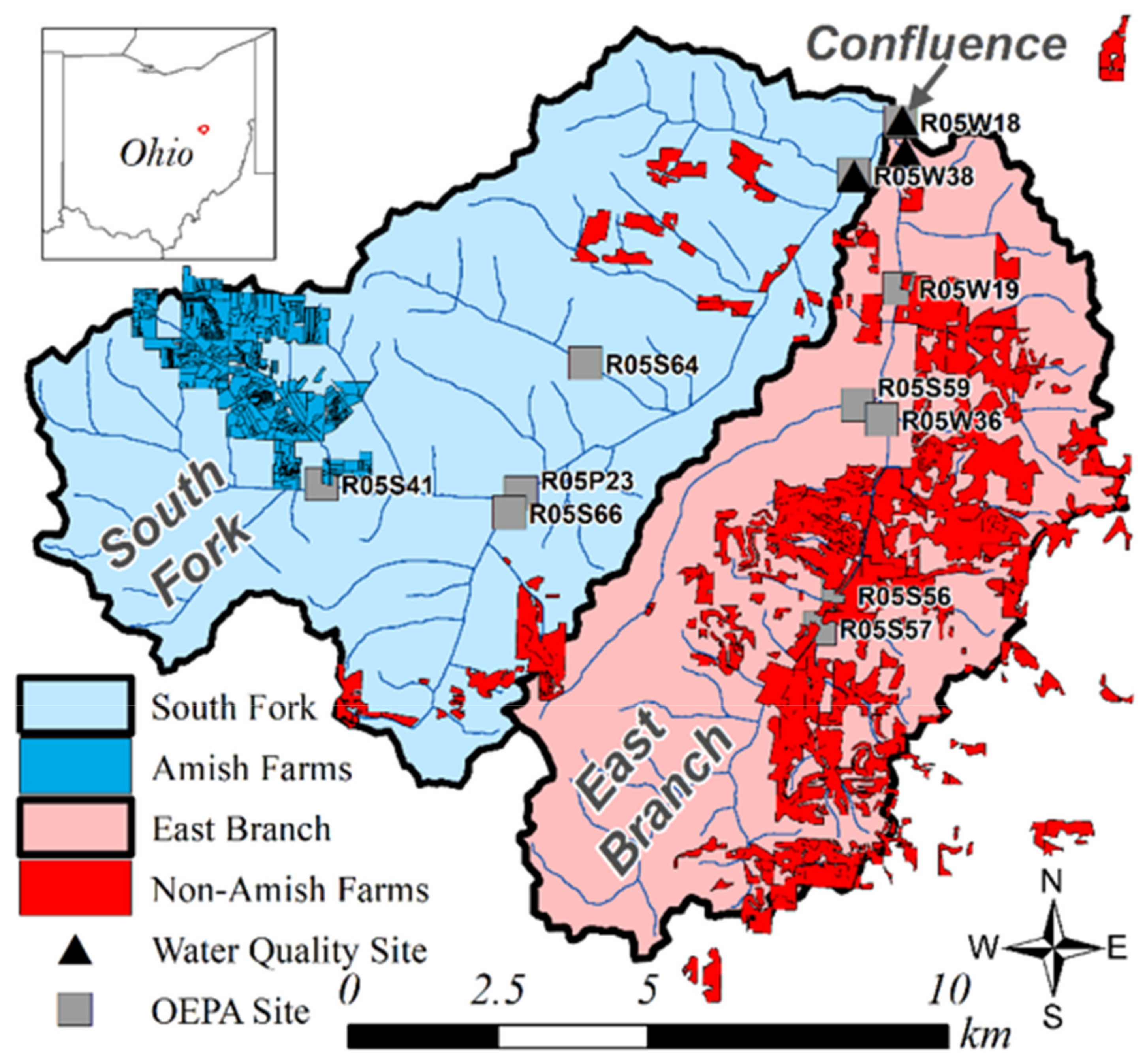
2.1.1. Sugar Creek, OH, USA: Two Culturally Distinct Sub-Watersheds

The Amish are a traditional agrarian Christian subculture that originated in Switzerland and Alsace in 1693 as an off-shoot of the Anabaptist branch of the Protestant Reformation [16,17]. Today, they can no longer be found in Europe. The North American Amish, located primarily in the states of Ohio, Pennsylvania, Iowa, and Indiana, preserve much of their Germanic heritage in a language that is an oral folk German dialect [18,19]. They have maintained a highly interconnected social system of cooperative, mutualistic, and unifying interactions which sustains them as a separate subculture. The primary unit of Amish society is a patriarchal family [20,21]. Groups of families are tightly connected as parts of an Amish church community or Gemeinde (a redemptive community [22], in which personal salvation takes place in the Christian community) who rotate for biweekly worship in each other’s homes and barns [18]. Each church community has its own lay church leaders and a set of socio–religious rules called the Ordnung, which create boundaries between them and the world and limit the scale of many aspects of their culture, including technology and farm operation [18,23,24]. For example, to encourage a slower pace of life and more local connectedness, Ordnungs do not allow church members to own automobiles; horses and buggies are used instead [18]. Furthermore, only horses are allowed to be the main source of power in agricultural field work so farm size is limited to what a family with a team of draft horses can manage (20–60 ha) [17,19,20]. There are also several small Amish parochial schools with education ending after the 8th grade. Cooperative labor in the form of oat threshing rings and corn silo filling rings is neighborhood-based and crisscrosses church boundaries. The Amish do not participate in USDA Farm Bill conservation programs, but a number of the Amish of the South Fork participated in the Alpine Nutrient Trading Plan which paid farmers for installing manure storage facilities and milk house waste underground storage tanks that are pumped out onto the fields. The South Fork Amish also installed conservation management practices on their dairy farms from several Ohio Environmental Protection Agency (OEPA) 319 grants, such as fencing cows out of streams. In 2016, the OEPA awarded Holmes County Soil and Water Conservation District a grant to eliminate manure and dairy parlor waste and improve or install heavy-use pads and access lanes, dairy cow exclusion fencing from streams, and alternate water sourcing to keep cows out of the streams.

The Amish settlement pattern in the South Fork clearly differs from the adjacent East Branch of the South Fork where the non-Amish dairy farmers live in separated larger farms. The Amish categorize the East Branch farmers as “English”, which, in the local community, means “non-Amish”, although most people in the East Branch have German–Swiss heritage. The East Branch dairy farmers are located upstream and downstream from the unincorporated town of Ragersville founded in 1830, which lies midway in the East Branch Valley. The town has a few buildings including a historical society building, a church, a tavern, and an elementary school. These farmers also frequent the Village of Sugar Creek. The farmers along the East Branch participated in an Ohio EPA 319 grant from 1995–1998 to deal with dairy waste separation and treatment. The East Branch dairy farmers primarily use manure lagoon pits. At that time there were 7800 cows among 16 diary operations in the 28.2 square mile East Branch watershed [25]. Later, they responded to the initial Sugar Creek Total Maximum Daily Load (TMDL) of 2002 by forming a cooperative to create a riparian buffer zone along the creek. They were also active in participating in cover crop programs provided by the Muskingum Watershed Conservancy District starting in 2013.

2.1.2. Two Modes of Dairy Farm Intensification

Two distinct modes of intensification evolved in the sub-watersheds. The Amish mode evolved mainly due to cultural decisions regarding the adoption of automatic milking machines instead of hand-milking, which resulted in a herd expansion relating to the extra time created for milking. The non-Amish dairy farmers primarily intensified by purposely expanding their herd size to take advantage of the economy of scale. These two modes of intensification are shown in

Table 1. A comparison of Amish South Fork and non-Amish East Branch modes of farming intensification.

Intensification Characteristics	Amish South Fork	East Branch
Type of Intensification	Automatic milking machines and herd expansion with land size constant	Land and herd size scale increase
Date of Major Intensification Starting Event	1996—Debate in each church district about social and economic values of hand versus automatic milking	1975—Agriculture vocational education teacher recommended scale increase for profit
Scale of Intensification	20% increase in herd size	200–500% herd increase; 2 CAFOs
Key Technological Changes	Milking machines; bulk tanks, solar electric fences, increase in off-farm inputs mainly for feed	Capital intensive dairy parlors; sand for bedding; round bales, silage hay; many off-farm inputs especially for feeding; high-yielding corn varieties
Key Land Use Changes	Increase in and conversion of pastures to intensive and rotational grazing by milking cows and heifers; increase in corn in the rotation	Pastures used only for dry cows and heifers; increase in cash cropping for corn or soybeans
Settlement Pattern	Small farms of about 80 acres with three generations living together, fissioning of church and small parochial school districts due to population increase	Larger farms of 200 to 1350 cows
Social Organizational Changes	Population increase; fissioning of church and school districts	Buffer and Manure Group formed; increase in hired labor

.

For dairy farm intensification processes in the South Fork of the Sugar Creek sub-watershed, Amish dairy intensification was triggered in the mid-1990s when the Old Order Amish church groups which milked cows by hand decided to allow milking machines. Prior to that, there was a high value on the family time together milking about 25 cows by hand on an average of 80 acres. Pioneering work on the ecological benefits of Amish self-sufficient farming was published by Deborah Stinner and Benjamin Stinner [26,27,28]. When the milking machines were allowed, it took much less time to milk. In most cases, by the late 1990′s, after the introduction of milking machines, steel bulk tanks were introduced so that the milk could be piped directly into one holding container that cooled the milk that could be picked up by a milk tank truck every two or three days. This replaced the need for 10-gallon milk cans which had been picked up daily. Owing to the labor time saved, most farms increased their herd size by about 10–20%. In turn, this necessitated more corn and hay to be grown to feed the cows, rotational grazing using solar-powered electric fences, and more permanent pasture grasses that were introduced to improve pasture yield, milk quality, and herd and soil health. The ideal Amish four-year five-crop rotation of corn, small grain such as spelt or barley, oats, and two years of hay was sometimes tweaked to add a second year of corn. Intensive grazing groups that used rotational paddocks became very popular as well, especially after 2011. New horse-drawn plows were invented to be able to plow the deeper roots of these grasses. While the increase in herd size contributed to an increase in manure production, the farmers were able to apply most of this to the increase in corn production which requires a higher fertilizer input.

A precondition for this mode of intensification was that the South Fork Amish population were socially circumscribed, resulting in a land shortage and an inability to increase the scale of farm acreage. In Clark Township, where the South Fork of Sugar Creek is located, there was a rapid population growth rate and a large family size of about five people per family during the study period, even though the birth rate had decreased substantially over the last 50 years. This is illustrated by the Amish church district settlement pattern of clustered farms and houses not just defined by the smaller farm size but also by the preference for living in a close community. Amish church districts usually divide when the number of households exceeds 40 to 45 to maintain their sense of community. In 1996, there were 156 church districts in Clark Township that had fissioned into 235 church districts by 2010 [29]. The preference by the Amish for single heir succession and inheritance of the farm results in a problem for non-inheriting children, most of whom cannot find farmland. In this case, they must find other jobs due to the shortage of land. This increase in the density of the South Fork Amish population has also resulted in the rapid seeding of new Amish communities in other places in Ohio and nearby states [30].

The intensification of dairy farms in the East Branch of the South Fork of the Sugar Creek began in 1975 when a local agricultural vocational education instructor in the high school taught that increasing the scale of farming would lead to increased farming profitability. At the time, this trend was popular in the United States and resulted in a rapid increase in large farms. This line of thinking focused on a scale that could be achieved either by owning or renting land along with an increase in herd size achieved with or without an increase of land. In the East Branch of the South Fork, the intensification included both an increase in farm acreage size, as well as herd size. It also meant that there was a large capital outlay for modern dairy parlors, sand for bedding, large round bales, hay used for silage, many off-farm inputs especially for feeding, and high-yielding varieties of GMO corn and soybeans sometimes used for cash cropping. Pastures were used only for dry cows and heifers. Because the increase in herd size was greater than the increase in land size, the farmers of the East Branch had an ongoing problem of excess manure. Two large dairy farms in the East Branch were Concentrated Agricultural Feeding Operations (CAFO). One had 1200 cows, 3000 acres, and 20 employees. When the current manager took it over from his father in 1978 there were only 140 cows. They went from 140 to 400 cows in 1980 by putting in a new free-stall barn. A new milking parlor was installed in 1992, enabling them to milk more cows and milk three times a day [31]. A second CAFO dairy with 1350 cows was run by a 5th generation family farm and a staff of 12 people. However, one hurdle that large capital-intensive farms continue to have is the possibility of fragmentation or dividing up the farm among multiple heirs in an equal inheritance system.

2.2. Farm Survey

Based on the general knowledge about the intensification of Amish and non-Amish dairy farming systems, we characterized how dairy intensification has led to two contrasting farming systems in terms of farm structure, animals, and crop management. In order to characterize the systems, we carried out a survey of farmers in both sub-watersheds, East Branch and South Fork, in the southern part of the Sugar Creek watershed.

Between 2005 and 2007, 17 Amish dairy farmers (3 in 2005–2006 and 14 in 2006–2007) and 11 non-Amish dairy farmers (11 in 2006–2007) were interviewed, collectively farming 494 ha and 2928 ha, respectively. Farmers were interviewed by the same person based on a semi-structured script. Interviews lasted one and a half hours up to three hours, depending on the size of the farm and the complexity of its management. Each interview dealt with:

(a)

The description of the main characteristics of the farm structure: land ownership, farm acreage composition by crops, hay, and other land uses; animal production on the farm including the number of animals per type; labor force on the farm.

(b)

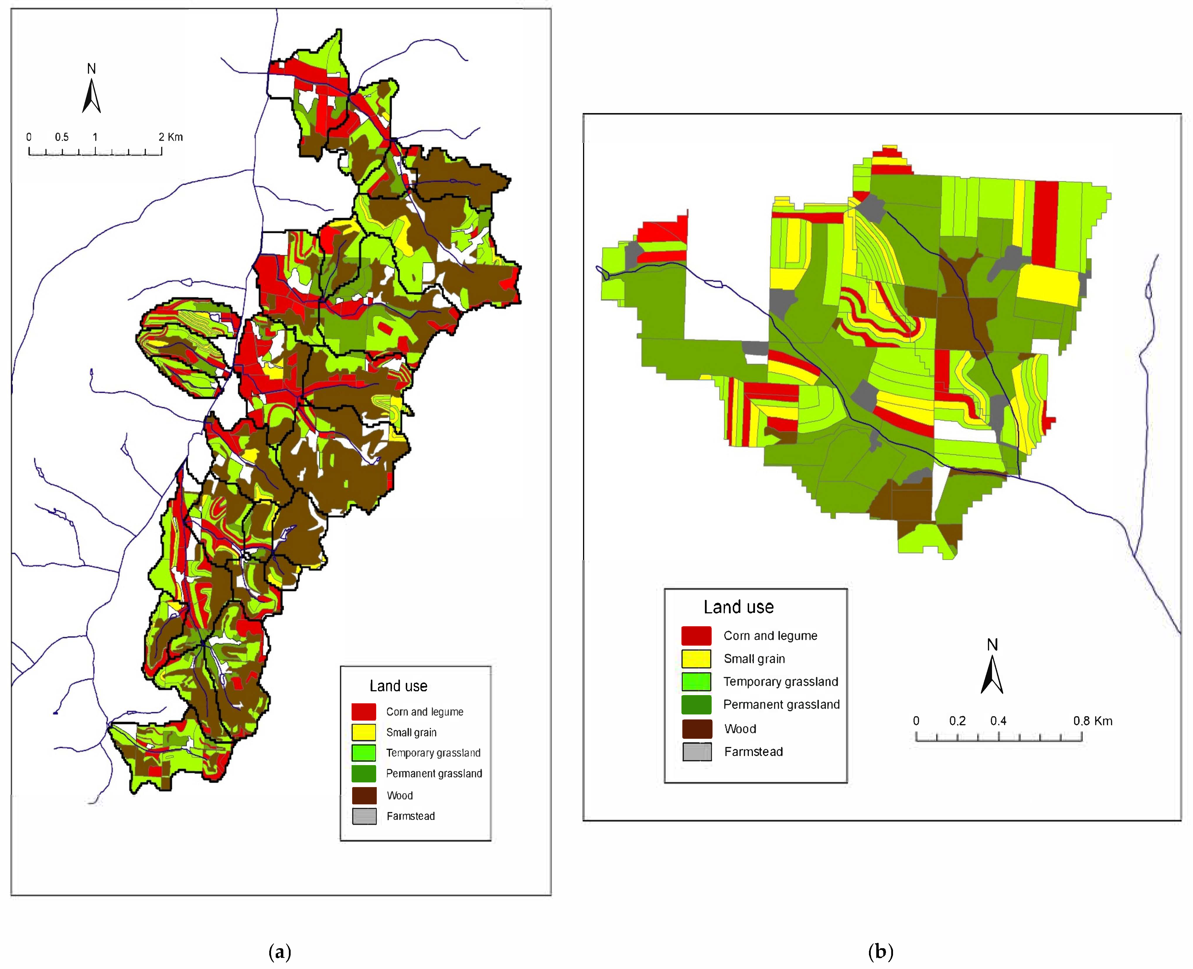
The identification of the farm territory: we define here the farm territory as the total fields managed by the farmer, including cropland, hayfields, and pasture. All the fields were reported on a map during the interviews with the farmers or when it was available checked on the maps established by the Farm Service Agency. Then a Geographical Information System (GIS) was created with all the fields of the farms surveyed. The land use for each field was collected for the cropping year 2006.

(c)

The land management through crop and animal management, where we focused on: (1) crop rotations and their spatial organization over the fields of the farm. For that, we utilized the methodologies described by Maxime et al. (1995) and Morlon and Benoit (1990) [32,33], which have already been explained and used in combination by Joannon et al. (2006) [34]; (2) animal feeding, as it has a direct impact on land management and explains partly the land use of the farm.

2.3. Water Data

2.3.1. Discharge Assessment

Given access and financial limitations, stream discharge was not measured within the study area but rather estimated from nearby sources. We downloaded mean daily discharge from seven United States Geological Survey stream gages within 50 km of the study area from 2010 to 2018 (Station IDs = 03139000, 03124500, 03116077, 03117000, 03117500, 03118500, 03140000) using the R package ‘dataRetrieval’ [35]. As stream discharge is affected by the watershed size, daily discharge was normalized between 0 and 1 using min–max normalization to remove the impact of watershed size. Following this procedure, the highest 25% and lowest 25% of daily discharge were isolated to assess trends in discharge and nutrient concentrations occurring during relatively high and low discharge periods. In addition, daily streamflow from each of the seven stream gages was normalized by watershed area to calculate area-weighted runoff. Daily runoff was aggregated by season and year to understand the general streamflow patterns over the study period.

The Regional Kendall Test (RKT) was used to determine significant trends (p < 0.05) in normalized daily discharge from 2010–2018 among the seven stream gages used in the analyses. In addition, the RKT was used to determine significant trends in the highest 25% (‘high discharge conditions’) and lowest 25% (‘low discharge conditions’) of daily normalized discharge among the seven stream gages. The RKT identifies trends at individual sites and compares the results among regions with no prior assumptions for normality [36]. Lag-1 autocorrelation coefficients were calculated to ensure data did not exhibit strong temporal autocorrelation. We used the R package ‘rkt’ to calculate the regional Kendall’s tau [37].

2.3.2. Water Quality Monitoring

Stream water nutrient concentrations were monitored approximately bi-weekly from 2010 to 2018 at the outlets of the East Branch of the South Fork of the Sugar Creek (‘East Branch’), South Fork of the Sugar Creek (‘South Fork’), and the combined downstream confluence (‘confluence’) as part of a nutrient trading plan (Figure 1; [38]). The East Branch drains an area slightly smaller (73 km²) compared to the South Fork (91 km²). Water samples were preserved in the field using 1 mL of 0.5 M sulfuric acid and filtered upon return to the lab using a 0.45 µm filter. Phosphate, total phosphorus, nitrate, ammonia, and total nitrogen concentrations were calculated using a Lachat QuickChem Flow Injection Analysis Automated Ion Analyzer (Hach Company, Loveland, CO, USA).

Mean nutrient concentrations for each site were calculated from all samples for the four sub-watersheds and compared to each other using the Tukey test. In addition, mean concentrations of samples collected during the high and low discharge conditions were also calculated and compared. The Kendal trend test was used to determine significant changes in nutrient concentrations among all the samples, and the samples collected during the high and low discharge conditions. Significance for all statistical tests was determined as being p < 0.05.

2.3.3. Habitat and Biological Assessments

Two surveys that evaluate stream health were conducted by the Ohio Environmental Protection Agency (OEPA): The Qualitative Habitat Evaluation Index (QHEI) and the Index of Biotic Integrity (IBI). The QHEI is a quantitative index that uses six physical riparian/stream variables to yield a numeric value for the stream’s habitat and is often used as a surrogate for the total suspended solids [39]. The OEPA determined from hundreds of samples that, in general, a QHEI score ≥60 is conducive for Warmwater Habitat use designation, the goal for most of Ohio’s rivers and streams, while scores less than 45 generally cannot support a Warmwater assemblage consistent with Warmwater Habitat biological criteria [39]. Here, Warmwater Habitat defines an aquatic life use designation assigned to an individual waterbody segment based upon the potential to support that use according to narrative and numerical criteria. The Index of Biotic Integrity (IBI), which is based on fish assemblage data, is one of the three indexes used by OEPA to evaluate Warmwater Habitat. The minimum IBI score required for Warmwater Habitat use designation is 40 for sites located in the Western Allegheny Plateau, the ecoregion containing the study sites [39].

The OEPA performed the QHEI and IBI at 11 sites in the South Fork Headwaters of Sugar Creek in 1998 and 2017 (Figure 1). Five sites each were located within the East Branch and South Fork watersheds, while the eleventh site was located at the confluence of the two streams. East Branch and South Fork QHEI and IBI scores were aggregated by watershed and tested for significant differences between watersheds using the Wilcox Rank Sum test for both 1998 and 2017. In addition, QHEI and IBI scores were also compared between years for each watershed to determine if significant changes in scores occurred between years for each watershed.

3. Results

3.1. Farm Survey

3.1.1. Farm Structure and Farming Systems

The main results are summarized in

Table 2. Production by farming type.

Production	Amish Watershed 1	Non-Amish Watershed
Dairy with milking cows	11 (2 with draft horses business)	5 (2 with cash crops/hay business)
Dairy with only heifers	1	2 (both with cash crops/hay business)
Poultry	1	none
Mixed livestock	none	1
Off-farm job, full time, with a Non-dairy production on-farm	4	3

¹ Based on the 14 farms surveyed and 3 of a previous study.

and

Table 3. Farms’ land use and animal raised.

Category	Amish Watershed 1	Non-Amish Watershed
Farmed land 2	16 to 54 (32)	14 to 747 (266)
Tillable land 2	0 to 35 (19)	5 to 731 (250)
Crops sold (% total land) 3	0 to 37% (5) 3	0 to 100% (7) 3
Number of milking cows 4	9 to 28 (23)	297 to 460 (310)
Level of production 5	6500 to 9440 (7182)	9000 to 13,500 (11,340)
Other livestock	Horses: 150 on 17 farms Chickens: 90,000 to 120,000 per year (3 farms)	1 mixed livestock (sold per year: lambs (65), beefs (105), hogs (650)

¹ Based on the 14 farms surveyed and 3 of a previous study. ² In ha; area range and average area in parenthesis. ³ In parenthesis the number of farmers concerned. ⁴ Range and average number in parenthesis, only for the farm concerned (see Table 2). ⁵ In kg/cow/year; range and average level in parenthesis.

. Most of the farms were dairy farms in both watersheds (68%), including farms raising only dairy heifers. The remaining operations were mainly associated with a full-time off-farm job of the main worker of the farm (25% of the farms surveyed). Other contrasting features of Amish and non-Amish are as follows. Amish farms were smaller than non-Amish (32 ha on average versus 266 ha), and for the dairy operations there were on average 23 milking cows in Amish farms and 310 in non-Amish farms. This is the direct consequence of animal traction used by Amish farmers which limits the maximum acreage a farmer and his family can cultivate. There was an average of nine horses per farm, Belgium/Percheron horses being used for traction and Standardbreds used for transportation. In the non-Amish watershed, farms associated with off-farm jobs were of comparable size as Amish farms. The level of milk production of non-Amish dairy farms was higher (11,340 vs. 7182 kg/cow/y), but some Amish and non-Amish farms had similar levels of production. Cash crops were cultivated more on non-Amish farms. The whole Amish farm was either owned by the farmer or rented out in the case of a young son who had not yet bought the farm from his father. Out of the twelve Amish farmers, just one had 36% of his farm rented out to another farmer, who was not his family. The main labor force was generally composed of the farmer and his wife with, for 58% of the farm, children helping on the farm. Moreover, corn silo filling and cereals threshing were shared with other farmers, most of the time with a group of six or seven farmers. On average, 58% of the non-Amish farmland was rented out, with a great diversity ranging from 24–84%. The labor force on these farms was composed of members of the family, permanent employees, and occasional helpers. On average there were 2.5 family members working on the farm (1 to 4.5), the farmer and/or his wife and/or brothers and/or sons. There were no permanent employees on the two dairy heifer farms, while there was an average of six permanent employees on dairy farms (from 2 to 9.5). Occasional helpers, who add another full-time permanent work position, were present on all the farms except one and typically worked during the summer or on evenings and weekends.

Cash crops were almost not cultivated on dairy Amish farms. For most of the Amish farms, all the fields were contiguous, or, at least, less than 500 m apart. The average field size was 1.4 ha with pasture fields being larger (2.4 ha on average) than hay and crop fields. On non-Amish farms, fields could be as far as 14 km from the farmstead. The average field size was 3.5 ha, which is larger compared to Amish farms, but small contour strips fields as small as 0.2 ha were also cultivated on these big dairy farms. The Amish used more than 95% of their land to produce animal feeds used on-farm, with on average 38% of pasture grazed, 32% in hayfields, 26% in small grain cereals fields, and less than 4% in cornfields. On non-Amish farms, there is on average less than 5% of pasture, 51% of hay, 28% of corn silage, and around 15% of small grain cereals.

3.1.2. Landscape Patterns and Crop Rotations

In Amish rotations the corn was cultivated for one or two years, followed by one year of oats and then by two to seven years of hay. Sometimes small grain cereals, such as spelt or barley, followed directly after the corn and before the oats. Rotations with two years of corn were localized on bottomland soil, which had more clay and could be flooded. On the hills, where the soil was sandier, better drained, and lower in water reserves, Amish farmers had rotations with a longer period of hay. Pasture fields were located either on the stonier fields or on fields too steep to be tilled and in the valley and along the streams because animals had direct access to water. Pasture was also preferentially located on the closest field to the barn.

For non-Amish dairy farms, the main rotation was also a succession of corn, small grain cereals, and hay, with a variation in the number of consecutive years each land use was kept before changing to the next one. There were also more specialized crop rotations: continuous corn, corn and soybeans, and continuous hay in rotation sometimes with a small grain to renew the grassland. These different specialized crop rotations were spatially organized on non-Amish farms as follows:

• on drained bottomland with water-logging constraint there was continuous corn or corn and soybean rotations;
• oppositely, on sandy hills there were continuous hayfields;
• on the remaining stony fields, and on fields too steep to be tilled there was pasture.

Finally, we aggregated land use information gained from our interviews to a watershed-level resolution by considering the spatial distributions of land cover within the direct drainage area of each farm interviewed. These maps of land use covering the zero and first-order stream systems demonstrate the differences in landscape patterns seen between the non-Amish (Figure 2a) and Amish (Figure 2b) sub-watershed. These aggregations help visualize the differences in farm management between the two sub-watersheds e.g. [40,41]: there is more pasture along the stream in the Amish watershed and more corn or wood in the non-Amish watershed.

3.2. Water Quality Results

3.2.1. Discharge Estimation

The mean annual area-weighted runoff for the seven USGS stream gages from 2010–2018 was 450 mm and ranged from 299 mm (2012) to 693 mm (2011). Winter (January–March) and spring (April–June) months were much wetter than summer (July–September) or fall (October–December) months. The mean seasonal runoff for winter, spring, summer, and fall was 161 mm, 145 mm, 53 mm, and 91 mm, respectively. March, on average, was the wettest month, producing 73 mm of runoff, followed by April (63 mm) and February (45 mm). The driest month, on average, was September (13 mm), followed by August (14 mm) and October (17 mm).

According to RKT results, daily stream discharge significantly increased in the seven nearby USGS stream gages analyzed (

Table 4. Regional Kendall Test results from seven nearby USGS stream gages for all stream discharge, the highest 25%, and the lowest 25% of stream discharge from 2010–2018. Significant positive Kendall’s tau indicates an increasing trend with time and significant negative Kendall’s tau indicates a decreasing trend with time. All trends were detected with significance at p < 0.05.

Variable	Kendall’s Tau	p-Value
All discharge	0.05	<0.001
Discharge >75%	−0.06	0.008
Discharge <25%	0.05	0.02

). Interestingly, RKT results indicated significant decreases in the highest 25% of stream discharge and a significant increase in the lowest 25% of stream discharge. Significant increases were detected during January, February, April, May, August, and November, while a significant decrease was measured during March.

3.2.2. Nutrient Concentrations

The mean stream water nutrient concentrations for all samples and samples collected during high and low discharge conditions are presented in

Table 5. Mean nutrient concentrations (mg/L) for phosphate, total phosphorus (Tot P), nitrate, ammonia, and total nitrogen (Tot N).

Site	Phosphate	Tot P	Nitrate	Ammonia	Tot N
All samples concentration (mg/L)
East Branch	0.115 c	0.167 b	2.315 a	0.349 a	3.246 a
South Fork	0.255 a	0.325 a	2.646 a	0.297 a	3.641 a
Confluence	0.183 b	0.246 ab	2.494 a	0.320 a	3.302 a
High discharge samples concentration (mg/L)
East Branch	0.142 a	0.205 a	3.488 a	0.417 a	4.838 a
South Fork	0.266 a	0.406 a	3.642 a	0.440 a	4.571 a
Confluence	0.207 a	0.319 a	3.673 a	0.391 a	4.420 a
Low discharge samples concentration (mg/L)
East Branch	0.125 b	0.176 b	1.011 b	0.411 a	1.875 b
South Fork	0.303 a	0.392 a	2.043 a	0.284 a	3.187 a
Confluence	0.202 ab	0.267 ab	1.469 b	0.365 a	2.310 b

Different letters next to the scores denote significantly different mean scores among the three sites using the Tukey test.

. Using all the samples available, phosphate and total phosphorus were significantly greater in the South Fork compared to the East Branch or confluence. However, nitrate, ammonia, and total N were similar for all three sites. Samples collected during high discharge conditions were not significantly different for any of the mean nutrient concentrations across the three sites. All nutrient concentrations except ammonia were significantly greater in the South Fork compared to the East Branch or confluence during low discharge conditions. Mean total phosphorus and nitrate concentrations typically exceeded OEPA’s recommend limits for obtaining Warmwater Habitat use designation for all sites (1.0 and 0.1 mg/L for nitrate plus nitrite and total phosphorus, respectively).

Results from the Kendal trend test for nutrient concentrations for all three sites are detailed in

Table 6. Kendall trend test results (Kendall’s tau) for phosphate, total phosphorus (Tot P), nitrate, ammonia, and total nitrogen (Tot N) among the three sites.

Site	Phosphate	Tot P	Nitrate	Ammonia	Tot N
All samples
East Branch	−0.01	0.19	0.03	−0.3	−0.02
South Fork	−0.19	−0.01	−0.04	−0.4	−0.08
Confluence	−0.15	0.03	−0.02	−0.35	−0.04
High discharge samples
East Branch	−0.32	−0.1	−0.27	−0.25	−0.37
South Fork	−0.25	−0.18	−0.29	−0.47	−0.37
Confluence	−0.37	−0.14	−0.27	−0.45	−0.3
Low discharge samples
East Branch	0.17	0.23	0.12	−0.22	−0.08
South Fork	−0.25	−0.19	0.05	−0.47	−0.06
Confluence	−0.13	−0.01	0.22	−0.39	0.1

Bold values indicate significant results (p < 0.05).

. When analyzing all of the samples, phosphate concentrations significantly decreased in the South Fork and the confluence. Total phosphorus concentrations significantly increased in the East Branch. No significant changes in nitrate or total nitrogen were observed at the three sites. Significant declines in ammonia concentrations were detected at all three sites.

Phosphate concentrations collected from high discharge condition samples significantly declined in the East Branch and the confluence, while total phosphorus did not significantly change for any of the three sites (Table 6). Total nitrogen concentrations from high discharge condition samples significantly declined at all three sites, while significant declines in ammonia were detected at the South Fork and confluence sites. Only the South Fork had significant declines in nitrate during high discharge conditions. Fewer significant changes in nutrient concentrations were observed from samples collected during low discharge conditions (Table 6). The South Fork indicated significant declines in phosphate and ammonia, while the confluence had significant declines in ammonia.

3.2.3. Habitat and Biological Assessments

Results from the OEPA IBI and QHEI surveys for 1998 and 2017 are shown in

Table 7. Index of Biotic Integrity (IBI) and Qualitative Habitat Evaluation Index (QHEI) results from the Ohio Environmental Protection Agency (OEPA) for the confluence and six sites each in the East Branch and South Fork for 1998 and 2017.

STORET	Watershed	IBI 1998	IBI 2017	QHEI 1998	QHEI 2017
R05W18	Confluence	29	34	48	50.8
R05S56	East Branch	24	40	42	50.5
R05S57	East Branch	24	28	45.5	54
R05S59	East Branch	24	30	31	39.5
R05W19	East Branch	26	36	23	52.5
R05W36	East Branch	22	32	44.5	46
	East Branch Mean	24 *	33.2 *	37.2 *	48.5 *,^
R05P23	South Fork	18	28	28.5	39.3
R05S41	South Fork	20	24	35.5	29.5
R05S64	South Fork	22	12	35	38
R05S66	South Fork	28	34	27	42
R05W38	South Fork	28	30	28.5	41.3
	South Fork Mean	23.2	25.6	30.9 *	38.02 *,^

Significant differences between mean survey scores for 1998 and 2017 in the East Branch and South Fork are denoted with *. Significant differences between East Branch and South Fork mean survey scores are denoted with ^.

. Both IBI and QHEI scores increased at most individual sites from 1998 to 2017, indicating stream habitat improvements that led to increased fish assemblage diversity. However, all individual sites are well below the recommended score (60) for obtaining Warmwater Habitat use designation. Similarly, all but one individual site had IBI scores less than the required level (40) for obtaining Warmwater Habitat use designation.

The mean IBI scores in the East Branch increased significantly from 1998 to 2017, while the mean QHEI scores increased significantly for both the East and South Fork. The mean IBI and QHEI scores were typically larger in the East Branch compared to the South Fork. However, significant differences were only detected for the QHEI in 2017.

4. Discussion

4.1. On the Complexity of the Concept of “Sustainable Intensification”

Pollution by organic nutrients to waterways is the main environmental issue in the Sugar Creek watershed; however, in these two modes of dairy farm intensification, we have documented both an improvement in water quality and an increase in milk production both per cow and per acre. Collectively, this could be considered “sustainable intensification”, achieved through significant efforts in both watersheds to reduce nutrient pollution (e.g., the Sugar Creek nutrient trading program, [42]). However, both cases have challenges remaining with regard to how sustainable the intensification truly is in the long run. For example, a challenge for all dairy farmers is the low price of milk which has ranged from USD 13 to USD 20 per cwt for the period 1980–2021 (except for 2007, 2012, and 2014, when it spiked higher) [6]. Because organic milk fetches nearly twice the price, several South Fork Amish farms have opted to go organic, although none have in the East Branch. It is remarkable that the smallholder South Fork Amish have been able to stay in business in an era when the median national trend per herd size rose from 80 in 1987 to 1300 in 2017 [6]. Perhaps the Amish have more flexibility both socially and in farm management. Most Amish farm families have side businesses that can be scaled up or down. In farm management, the small field size makes adjusting the crop rotation or which fields to plant first easier than on large-scale farms.

Following the years of our study from 2018–2021, the total number of livestock decreased in both watersheds mainly owing to the better job opportunities in the area and low milk prices. Because of the low milk prices, a few Amish farms stopped dairy production and instead raised dogs, started side woodworking companies, or commuted to jobs in nearby towns. In the East Branch, one of the two CAFOs went out of business mainly due to succession issues regarding multiple heir ownership.

For the Amish, another issue is the population rate of increase that is forcing further divisions of their church districts and small parochial schools all the while keeping the number of farms at a fairly constant number through single heir succession. Despite the low milk prices, most Amish households have been able to have one or more household members work off the farm or start an on-farm side business. The Amish also have their own private health care insurance [43,44] which is a problem for many non-Amish “English” farm families. For the East Branch dairy farmers, most families have a family member working off the farm in large part to gain the insurance benefit. The East Branch dairy farmers also have a significant manure surplus problem that has not been resolved to date. The East Branch farmers have favored using more GMO corn and soybean varieties and more external inputs than the Amish dairy farmers. The Amish solved their manure surplus created from the dairy cow herd increase through nutrient cycling of the increased manure onto the increased corn acreage.

Taken altogether, what emerges is the complexity of the concept of “sustainable intensification” in practice when considering a working landscape where humans work as responsible members of a natural ecosystem. As we consider the pillars of the economy, society, and the environment as they pertain to sustainability and water resource management, we clearly need to explicitly consider socio–cultural dimensions in order to understand development impacts as they pertain to sustainability in these intensifying working landscapes. We outline the mechanisms driving such considerations as they pertain to our current study through the lens of water quality and implementation of agricultural management practices in the following.

4.2. Potential Organic Nutrient Pressure on Streams from Farms

We made an analysis of all the farms surveyed in this study, calculating the potential organic nutrients (nitrogen and phosphorus) that could impact streams during a year by the animals raised on the farm as a simple mass balance. For the calculation, we used French reference values [45,46,47,48] which have already been used in similar estimations to give the amount of organic nitrogen and phosphorous excreted for each type of animal [49]. We then calculated the two ratios, N/ha and P₂O₅/ha, for all the farms surveyed (

Table 8. Potential organic nutrients released at the farm level for the 11 non-Amish farms (NA) and 17 Amish farms (A) according to the ration of P₂O₅ and N organic produced by the animals raised on the farm divided by the acreage of the farm.

		kg P2O5/ha
		0–15	15–30	30–45	45–60	60–75	+140
N kg/ha	0–25	2 NA
	25–50		3 A/1 NA
	50–75		2 A/2 NA	2 A/1 NA
	75–100			5 A/2 NA
	100–125				2 A/2 NA
	125–150					1 NA
	+290						3 A

), which demonstrates that (1) two non-Amish farms had the lowest ratios close to zero—these are farms with no or few animals; (2) oppositely, there were three Amish farms with very high ratios over 290 kg/ha for nitrogen and 140 kg/ha for phosphorus—the three farms had large chicken houses; and (3) in between these extremes there were 23 Amish and non-Amish farms with a moderate-low to moderate-high ratio, and no major differences between Amish and non-Amish can be found.

The main result of this analysis is that we cannot distinguish between Amish and non-Amish dairy farms through this mass balance estimation as both have similar nutrient mass estimates and could have equal impact on water quality. This result agrees with a study that took place in Holmes County, OH, USA in a region dominated by Amish farms and which is the same county where we interviewed Amish farmers for our current study [50]. This previous work showed that Amish farming systems could rely on rather high amounts of imported animal feed, which may cause some environmental problems with nutrient loading, especially phosphorus. However, both Amish and non-Amish systems had rather low nitrogen ratios. Indeed, the nitrogen ratio calculated on 139 dairy farms across nine European dairy areas was usually over 125 kg/ha [51], while this was the case for only 1 dairy farm out of the 19 in our study.

4.3. Potential Role of Manure Storage and Application

Amish farms had all their fields close to the farmstead while non-Amish farms cultivated land far from their farmstead. This can lead to a non-homogeneous manure application, with a disproportionate spreading close to the farmstead and distant fields having less or no manure applied [52,53]. This is confirmed by the fact that a surplus of manure has been a major environmental issue within the non-Amish East Branch sub-watershed (personal communication, Tuscarawas Soil and Water Conservation District, OH, USA).

Considering manure storage capacity, non-Amish farms had larger storage facilities which allowed them to haul manure at a more appropriate time to take advantage of crop requirements and weather conditions. This improvement of manure storage in lagoons on non-Amish farms is related to the manure surplus issue as stated above. Amish farms tended to apply straw pack (semi-composted) manure earlier than non-Amish farms, which sometimes presented a problem when it was applied to land that was still freezing and thawing in early spring. This way of managing manure is similar to what has been observed among Amish farmers in Wisconsin [54].

4.4. Impact of Farming Systems and Management on Stream Water Quality

Nutrient concentrations in stream water samples collected from 2010 to 2018 at the outlets of the two sub-watersheds were significantly different during low discharge conditions but were similar during high discharge (Table 5). Nutrient concentrations measured during high discharge conditions likely contributed the most to annual nutrient loads and suggest the two different types of farming practices employed in the adjacent sub-watersheds of Sugar Creek have a similar impact on annual nutrient loads. The different landscape patterns observed in the adjacent sub-watersheds likely contributed to these observations (Figure 2). While the non-Amish sub-watershed tended to have continuous corn cropping with manure application along streams in riparian areas, there was also a greater tendency for riparian woodland buffers that could have allowed space and time for nutrient uptake to occur before being transported to the streams. Conversely, in the Amish sub-watershed grass, stream buffers were more common. However, livestock was not fenced away from streams, which could have balanced out the positive effect of the grass buffers.

Differences in nutrient concentrations measured during low discharge periods may reflect legacy nutrient contributions from older groundwater sources influenced by previous farming practices. For example, in the South Fork, livestock was historically allowed to graze in the stream, which could create elevated nutrient concentrations in riparian soils that were most apparent during low discharge conditions when contributions from stormflow were negligible. During low discharge conditions, the East Branch had significantly lower concentrations for all nutrients except for ammonia.

Changes in water quality implied from nutrient concentration trend tests and comparison of the IBI and QHEI assessments suggest water quality has improved in both sub-watersheds, but additional improvements are still needed to obtain recommended scores for obtaining Warmwater Habitat use designation. While the mean IBI score did not significantly increase in the South Fork from 1998 to 2017, the score from one site located immediately downstream from a cheese production plant that discharges nutrient-rich effluent (R05S64) heavily impacted the result—removing this site would have resulted in a significant increase in mean IBI score for the South Fork. Attributing the changes in the observed stream water nutrient concentrations or biological and habitat assessments to the different farming practices is difficult due to the many factors that could have affected these observations. For example, dozens of best management practices aimed to reduce erosion and subsequent nutrient loss from farm fields were installed in the Amish sub-watershed during the study period [38,55,56].

5. Conclusions

Two very different rural populations in two adjacent sub-watersheds have intensified their dairy farming systems in two completely different ways. Differences concern the size of the farms and the herds, the level of production, the way to feed dairy cows, the spatial patterns of fields, crop uses and rotations, and the demographics of the populations themselves. Several previous studies [18,26] about Amish dairy production have focused on either the social or natural/biological aspects exclusively and therefore result in an oversimplified description of Amish agriculture as a sustainable way of farming especially as it relates to water quality [57,58]. Our estimation of potential organic nutrient loads to the streams, along with the other characteristics of both farming systems, do not allow us to conclude whether or not Amish farmers currently have less impact on the environment than their non-Amish counterparts. Further, while both systems increased milk production substantially and improved water quality when considering some aspects, meeting the definition of “sustainable intensification” presented in the introduction, our findings are insufficient to conclude that both systems reached “sustainable intensification” in any true sense. To do so would require more transdisciplinary research on external inputs, externalities including greenhouse gas emissions, carbon sequestration, biodiversity, yield gaps, and long-term social factors such as the difference in inheritance and succession patterns and human and social capital (e.g., [59,60]). Our results indicate the need for a more complex analysis incorporating both social and natural sciences when assessing and evaluating “sustainable intensification” especially as it pertains to and impacts on water resource management.

References

1. Clay, N.; Garnett, T.; Lorimer, J. Dairy intensification: Drivers, impacts and alternatives. Ambio 2020, 49, 35–48. [Google Scholar] [CrossRef] [Green Version]
2. Pretty, J.; Bharucha, Z.P. Sustainable intensification in agricultural systems. Ann. Bot. 2014, 114, 1571–1596. [Google Scholar] [CrossRef]
3. Blayney, D.P. Electronic Report from the Economic Research Service the Changing Landscape of U.S. Milk Production; USDA: Washington, DC, USA, 2002. [Google Scholar]
4. USDA. Milk Production; USDA: Washington, DC, USA, 2018. [Google Scholar]
5. FAO. Dairy and dairy products. In OECD-FAO Agricultural Outlook 2018–2027; FAO: Rome, Italy, 2018; pp. 178–189. [Google Scholar]
6. Macdonald, J.M.; Law, J.; Mosheim, R. Consolidation in U.S. Dairy Farming United States Department of Agriculture; USDA Economic Research Service, Economic Research Report; USDA: Washington, DC, USA, 2020. [Google Scholar]
7. Thompson, P.B. (Ed.) The Ethics of Intensification: Agricultural Development and Cultural Change; Springer: Dordrecht, The Netherlands, 2008; ISBN 978-1402087219. [Google Scholar]
8. Millennium Ecosystem Assessment. Ecosystems and Human Well-Being: Synthesis; Island Press: Washington, DC, USA, 2005. [Google Scholar]
9. Mbow, C.; Rosenzweig, C. Food security. In Climate Change and Land: An IPCC Special Report on Climate Change, Desertification, Land Degradation, Sustainable Land Management, Food Security, and Greenhouse Gas Fluxes in Terrestrial Ecosystems; IPCC: Geneva, Switzerland, 2019; pp. 1–864. [Google Scholar]
10. Matson, P.A.; Parton, W.J.; Power, A.G.; Swift, M.J. Agricultural intensification and ecosystem properties. Science 1997, 277, 504–509. [Google Scholar] [CrossRef] [Green Version]
11. Lin, B.B.; Perfecto, I.; Vandermeer, J. Synergies between agricultural intensification and climate change could create surprising vulnerabilities for crops. Bioscience 2008, 58, 847–854. [Google Scholar] [CrossRef] [Green Version]
12. Altieri, M.A. Agroecology: The Science of Sustainable Agriculture, 2nd ed.; CRC Press: Boca Raton, FL, USA, 1995; ISBN 9780429495465. [Google Scholar]
13. Gliessman, S.R. Agroecology: Ecological Processes in Sustainable Agriculture; CRC Press: Boca Raton, FL, 1998; ISBN 9781575040431. [Google Scholar]
14. Society, R. Reaping the Benefits: Science and the Sustainable Intensification of Global Agriculture; The Royal Society: London, UK, 2009. [Google Scholar]
15. Liao, C.; Brown, D.G. Assessments of synergistic outcomes from sustainable intensification of agriculture need to include smallholder livelihoods with food production and ecosystem services. Curr. Opin. Environ. Sustain. 2018, 32, 53–59. [Google Scholar] [CrossRef]
16. United Nations Statistics Division (UNSD). Global Indicator Framework for the Sustainable Development Goals and Targets of the 2030 Agenda for Sustainable Development. Available online: https://unstats.un.org/sdgs/indicators/Global%20Indicator%20Framework%20after%202022%20refinement_Eng.pdf17 (accessed on 3 March 2022).
17. Smith, H.C. The Story of the Mennonites, 4th ed.; Mennonite Publication Office: Newton, Kansas, 1957. [Google Scholar]
18. Hostetler, J.A. Amish Society; Johns Hopkins University Press: Baltimore, MA, USA, 1993; ISBN 9780801844423. [Google Scholar]
19. Buffington, A.F. Pennsylvania German: Its Relation to Other German Dialects. In American Speech; Duke University Press: Durham, NC, USA, 1939; pp. 276–286. [Google Scholar]
20. Huntington, A.G.E. Dove at the Window: A Study of an Old Order Amish Community in Ohio; Yale University: New Haven, CT, USA, 1957. [Google Scholar]
21. Schreiber, W.I. The Hymns of the Amish Ausbund in Philological and Literary Perspective. Mennon. Q. Rev. 1962, 36–60. [Google Scholar]
22. Cronk, S.L. Gelassenheit: The rites of the redemptive process in Old Order Amish and Old Order Mennonite communities. Mennon. Q. Rev. 1981, 55, 5–44. [Google Scholar]
23. Kuhns, L. Modern farming technology and its ominous pose to the Amishman’s society. Small Faring J. 1989, 13, 20–22. [Google Scholar]
24. Kline, D. Great Possessions: An Amish Farmer’s Journal; North Point Press: San Francisco, CA, USA, 1990; ISBN 9781466825192. [Google Scholar]
25. McKinney, A. Dewatering Dairy Manure Using Polymer and Belt Press Technology. In Proceedings of the Manure Management in Harmony with the Environment Conference 1998, New Philadelphia, OH, USA, 10–12 February 1998. [Google Scholar]
26. Stinner, D.H.; Paolette, M.G.; Stinner, B.R. Amish Agriculture and Implications for Sustainable Agriculture. Agric. Ecosyst. Environ. 1989, 27, 77–90. [Google Scholar] [CrossRef]
27. Stinner, D.H.; Glick, I.; Stinner, B.R. Forage legumes and cultural sustainability: Lessons from history. Agric. Ecosyst. Environ. 1992, 40, 233–248. [Google Scholar] [CrossRef]
28. Stinner, D.H.; Stinner, B.R.; Martsolf, E. Biodiversity as an organizing principle in agroecosystem management: Case studies of holistic resource management practitioners in the USA. Agric. Ecosyst. Environ. 1997, 63, 199–213. [Google Scholar] [CrossRef]
29. Long, S.E.; Moore, R. Amish Church District Fissioning and Watershed Boundaries among Holmes County, Ohio, Amish. J. Amish Plain Anabapt. Stud. 2015, 2, 186–202. [Google Scholar] [CrossRef] [Green Version]
30. Donnermeyer, J.F.; Anderson, C.; Cooksey, E.C. The Amish Population: County Estimates and Settlement Patterns. J. Amish Plain Anabapt. Stud. 2013, 1, 72–109. [Google Scholar] [CrossRef] [Green Version]
31. Wagoner, R. Ohio family carries weight of large-scale dairy farming. The Lima News, 18 February 2020. [Google Scholar]
32. Maxime, F.; Mollet, J.-M.; Papy, F. Aide au raisonnement de l’assolement en grande culture. Cah. Agric. 1995, 4, 351–362. [Google Scholar]
33. Morlon, P.; Benoit, M. Étude méthodologique d’un parcellaire d’exploitation agricole en tant que système. Agronomie 1990, 6, 499–508. [Google Scholar] [CrossRef]
34. Joannon, A.; Souchère, V.; Martin, P.; Papy, F. Reducing runoff by managing crop location at the catchment level, considering agronomic constraints at farm level. L. Degrad. Dev. 2006, 17, 467–478. [Google Scholar] [CrossRef]
35. De Cicco, L.A.; Hirsch, R.M. The dataRetrieval R Package; U.S. Geological Survey: Reston, VA, USA, 2014; pp. 1–26. [Google Scholar]
36. Helsel, D.R.; Frans, L.M. Regional Kendall test for trend. Environ. Sci. Technol. 2006, 40, 4066–4073. [Google Scholar] [CrossRef]
37. Marchetto, A. Mann-Kendall Test, Seasonal and Regional Kendall Tests. Available online: https://cran.r-project.org/package=rkt (accessed on 1 May 2022).
38. Miller, S.A.; Lyon, S.W.; Moore, R.H. Impacts of a nutrient trading plan on stream water quality in Sugar Creek, Ohio. J. Am. Water Resour. Assoc. Rev. 2021. In press. [Google Scholar]
39. OEPA. Total Maximum Daily Loads for the Sugar Creek Basin; OEPA: Columbus, OH, USA, 2002. [Google Scholar]
40. Le Ber, F.; Benoit, M. Review article Methods for studying root colonization by introduced. Agronomie 1998, 18, 103–115. [Google Scholar] [CrossRef] [Green Version]
41. Thenail, C.; Baudry, J. Variation of farm spatial land use pattern according to the structure of the hedgerow network (bocage) landscape: A case study in northeast Brittany. Agric. Ecosyst. Environ. 2004, 101, 53–72. [Google Scholar] [CrossRef]
42. Moore, R. The Role of Water Quality Trading in Achieving Clean Water Objectives. Written Testimony. 2014, US Congress House of Representatives Transportation Committee on Water Resources. Hearing on Water Quality Trading, March 25, 2014. In The Role of Water Quality Trading in Achieving Clean Water Objectives Published by the United States Congress. Available online: https://docs.house.gov/meetings/PW/PW02/20140325/101952/HHRG-113-PW02-Wstate-MooreR-20140325.pdf (accessed on 15 March 2022).
43. Rohrer, K.; Dundes, L. Sharing the Load: Amish Healthcare Financing. Healthcare 2016, 4, 92. [Google Scholar] [CrossRef] [Green Version]
44. Becot, F.; Inwood, S.; Bendixsen, C.; Henning-Smith, C. Health Care and Health Insurance Access for Farm Families in the United States during COVID-19: Essential Workers without Essential Resources? J. Agromed. 2020, 25, 374–377. [Google Scholar] [CrossRef]
45. Corpen. Estimation des Flux D’azote, de Phosphore et de Potassium Associés aux Vaches Laitières et à Leur Système Fourrager; Corpen: Paris, France, 1999. [Google Scholar]
46. Corpen. Estimation des Flux D’azote, de Phosphore et de Potassium Associés aux Bovins Allaitants et aux Bovins en Croissance ou à L’engrais, Issus des Troupeaux Allaitants et Laitiers, et à Leur Système Fourrager; Corpen: Paris, France, 2001. [Google Scholar]
47. Corpen. Estimation des Rejets D’azote-Phosphore-Potassium-Cuivre et Zinc des Porcs; Corpen: Paris, France, 2003. [Google Scholar]
48. Corpen. Estimation des Rejets D’azote, Phosphore, Potassium, Cuivre, Zinc par les Élevages Avicoles; Corpen: Paris, France, 2006. [Google Scholar]
49. Basset-Mens, C.; Van Der Werf, H.M.G. Scenario-based environmental assessment of farming systems: The case of pig production in France. Agric. Ecosyst. Environ. 2005, 105, 127–144. [Google Scholar] [CrossRef]
50. Bender, M.H. Animal production and farm size in Holmes County, Ohio, and US agriculture. Am. J. Altern. Agric. 2003, 18, 70–79. [Google Scholar] [CrossRef]
51. Bossuet, I.; Chambaut, H.; Raison, C.; Le Gall, A. Green Dairy: Environment Friendly and Sustainable Dairy Systems in the Atlantic Area—Action A: Study of Mineral Flows on Dairy Systems in Experimental Farms. Report of the 2004–2005 Campaign; Institut de l’Élevage: Paris, France, 2005. [Google Scholar]
52. McKinney, A. East Branch Watershed Management Plan; Philadelphia Water Department Tookany: New Philadelphia, OH, USA, 2002. [Google Scholar]
53. Powell, J.M.; Jackson-Smith, D.B.; McCrory, D.F.; Saam, H.; Mariola, M. Nutrient management behavior on Wisconsin dairy farms. Agron. J. 2007, 99, 211–219. [Google Scholar] [CrossRef] [Green Version]
54. Brock, C.; Barham, B. Farm structural change of a different kind: Alternative dairy farms in Wisconsin—Grazers, organic and Amish. Renew. Agric. Food Syst. 2009, 24, 25–37. [Google Scholar] [CrossRef]
55. Souchere, V.; Cerdan, O.; Bissonnais, Y.L.; Couturier, A.; King, D.; Papy, F. Incorporating Surface Crusting and its Spatial Organization in Runoff and Erosion Modeling at the Watershed Scale. In Sustaining the Global Farm: Selected Papers from the 10th International Soil Conservation Orgainization Meeting, Proceedings of the 10th International Soil Conservation Organization Meeting, West Lafayette, IN, USA, 24–29 May 1999; Purdue University: West Lafayette, IN, USA, 2001; pp. 888–895. [Google Scholar]
56. Ohio EPA. Total Maximum Daily Loads for Bacteria for the Sugar Creek Watershed; OEPA: Columbus, OH, USA, 2007. [Google Scholar]
57. Ulrich-Schad, J.D.; Brock, C.; Prokopy, L.S. A Comparison of Awareness, Attitudes, and Usage of Water Quality Conservation Practices Between Amish and Non-Amish Farmers. Soc. Nat. Resour. 2017, 30, 1476–1490. [Google Scholar] [CrossRef]
58. Iles, K.; Ma, Z.; Erwin, A. Identifying the common ground: Small-scale farmer identity and community. J. Rural. Stud. 2020, 78, 25–35. [Google Scholar] [CrossRef]
59. Jordan, N.R.; Davis, A.S. Middle-way strategies for sustainable intensification of agriculture. BioScience 2015, 65, 513–519. [Google Scholar] [CrossRef] [Green Version]
60. Vasco Silva, J.; Reidsma, P.; Baudron, F.; Laborte, A.G.; Giller, K.E.; van Ittersum, M.K. How sustainable is sustainable intensification? Assessing yield gaps at field and farm level across the globe. Glob. Food Secur. 2021, 30, 100552. [Google Scholar] [CrossRef]
Figure 1. Map of the South Fork of the Sugar Creek (South Fork; blue) and East Branch of the South Fork of the Sugar Creek (East Branch; red) showing the location of streams, Ohio Environmental Protection Agency (OEPA) habitat survey sites with STORET labels, and water quality monitoring sites. The location of Amish (blue) and non-Amish (red) farms that have been surveyed in this study are overlaid on the two sub-watersheds. Water quality and habitat conditions were also monitored downstream of two watersheds at the confluence. The location of the study area within the State of Ohio is shown in the top left and bounded by a box with a north-west corner at 40°31′19″, 81°46′28″ and a south-east corner at 40°24′19″, 81°35′28″.
Sustainability 14 06201 g001
Figure 2. (a) Land use map aggregated at the watershed level (from the non-Amish farm interviews watershed). (b) Land use map aggregated at the watershed level from the Amish farm interviews.
Sustainability 14 06201 g002