
Formulation of Radiometric Calibration for Azimuthal Multi-Angle Observation Space-Borne SAR

1
School of Electronics and Information Engineering, Beihang University, Beijing 100191, China
2
Beijing Institute of Remote Sensing Information, Beijing 100192, China
*
Author to whom correspondence should be addressed.
Sustainability 2022, 14(11), 6757; https://0-doi-org.brum.beds.ac.uk/10.3390/su14116757
Submission received: 29 April 2022
/
Revised: 28 May 2022
/
Accepted: 30 May 2022
/
Published: 31 May 2022
(This article belongs to the Special Issue Applications of Advanced Remote Sensing Technology for Sustainable Resource Exploration and Assessment)
Abstract
:A novel space-borne SAR technique, azimuthal multi-angle observation (AMAO), has recently been proposed. It has highly flexible working modes and powerful capability of target information acquisition, but has challenges in achieving radiometric measurement accuracy. The larger the squint angle, the higher the resolution and the more variations involved. Radiometric calibration is a necessary approach to consistent and accurate SAR measurements, but has so far not been carefully considered for AMAO space-borne SAR. This paper addressed the new issues in radiometric calibration arising from the AMAO space-borne SAR system. The AMAO imaging modes are firstly been illustrated, based on which the influences of the AMAO on radiometric calibration are analyzed. To guarantee the accuracy of the radiometric calibration, an appropriate form of the SAR radar equation is derived for AMAO space-borne SAR. On these bases, the calibration models can be obtained by reformulating the novel AMAO SAR equation, and the corresponding normalization method is then proposed. The good experimental performance indicators verify the correctness of proposed models and the effectiveness of the correction method.
1. Introduction
Synthetic aperture radar (SAR) achieves high-resolution day-and-night observations in almost all weather conditions. Early space-borne SARs worked with the antenna broadside beam and then used multiple elevation beams to expand the imaging area. Today’s state-of-the-art space-borne SARs already have some azimuthal beam-steering capability, enabling high resolution or wide swath through innovative imaging modes, such as the sliding Spotlight, staring Spotlight, wrapped staring spotlight, TOPSAR, inverse TOPSAR, and bidirectional SAR [1,2,3,4,5,6]. In recent years, based on the ever-improving azimuthal beam-steering capability, a novel azimuthal multi-angle observation (AMAO) space-borne SAR technique was proposed in [7], and related researches were carried out in [8,9,10,11,12,13,14]. Utilizing highly flexible antenna beams, the AMAO space-borne SAR can effectively acquire rich multi-angle information for detailed analysis of high-value targets, three-dimension location, moving target detection, and velocity estimation.
Accurate calibration is necessary for quantitative comparison and analysis between multi-angle images. Physical quantities, such as (normalized) radar cross section (RCS), can be derived from calibrated SAR images for quantitative geophysical applications. AMAO brings not only the advantage of rich information acquisition but also new challenges to radiometric calibration, especially in the case of high squint and high resolution. The higher the squint angle, the longer the synthetic aperture, and the greater the radiometric variations. Consequently, the radiometric inconsistency from AMAO requires detailed analysis and precise normalization.
This paper focuses on the formulation of radiometric calibration in the case of AMAO space-borne SAR. First, the new challenges posed by the novel AMAO technique to SAR radiometric calibration are analyzed. Next, an appropriate form of the SAR radar equation is derived for AMAO space-borne SAR. On these bases, models of radiometric normalization are established, and the correction methods are subsequently given. Finally, experiments are conducted to verify the precision of the proposed models and the effectiveness of the correction method.
The rest of this paper is organized as follows: the problems of calibration arising from AMAO are analyzed in Section 2. The radar equation is extended in Section 3 for the radiometric measurements of AMAO space-borne SAR. The models and methods of radiometric normalization are given in Section 4. Experiments are performed in Section 5. Some discussions of the proposed models and the results are shown in Section 6, and the conclusions are summarized in Section 7.
2. Calibration Challenges for AMAO Space-Borne SAR
2.1. AMAO Space-Borne SAR Imaging
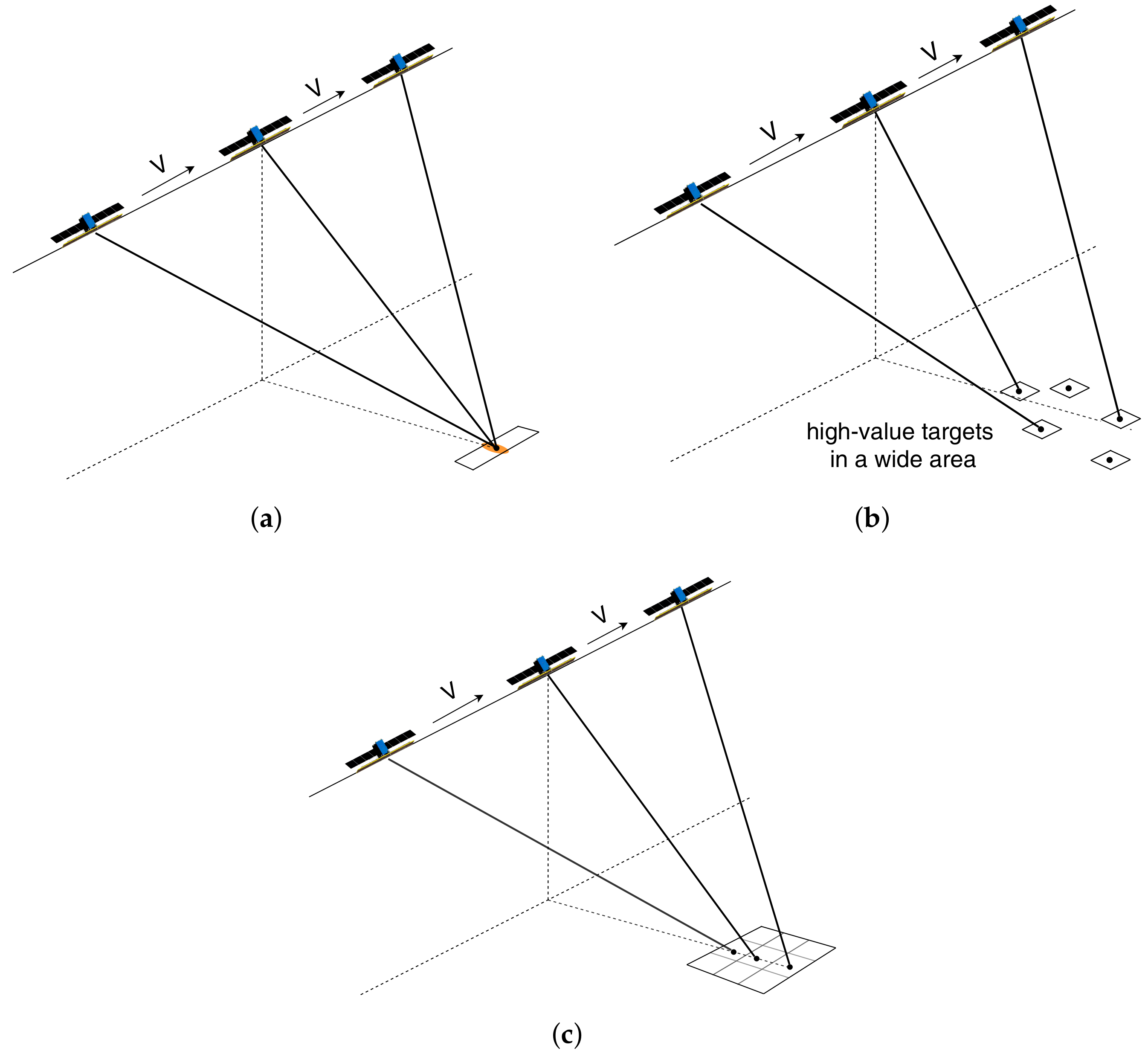
The AMAO space-borne SAR technique greatly improves the flexibility, efficiency, and information content of observation by utilizing the powerful beam-steering capability. Figure 1 illustrates AMAO imaging modes. Figure 1a shows the detailed target observation using long-exposure Spotlight mode, which acquires image sequences from multiple azimuth directions in a single flight for detailed analysis of high-value targets, three-dimension location, moving target detection, and velocity estimation. Figure 1b shows the multi-target observation mode. Unlike the conventional broadside SAR, which can only image one of the targets in the same range direction within a single pass, AMAO SAR can observe multiple targets, greatly improving the observation flexibility and revisit time. Figure 1c shows the high-resolution wide-swath mode, which is achieved by azimuth beam steering combined with TopSAR or mosaic.
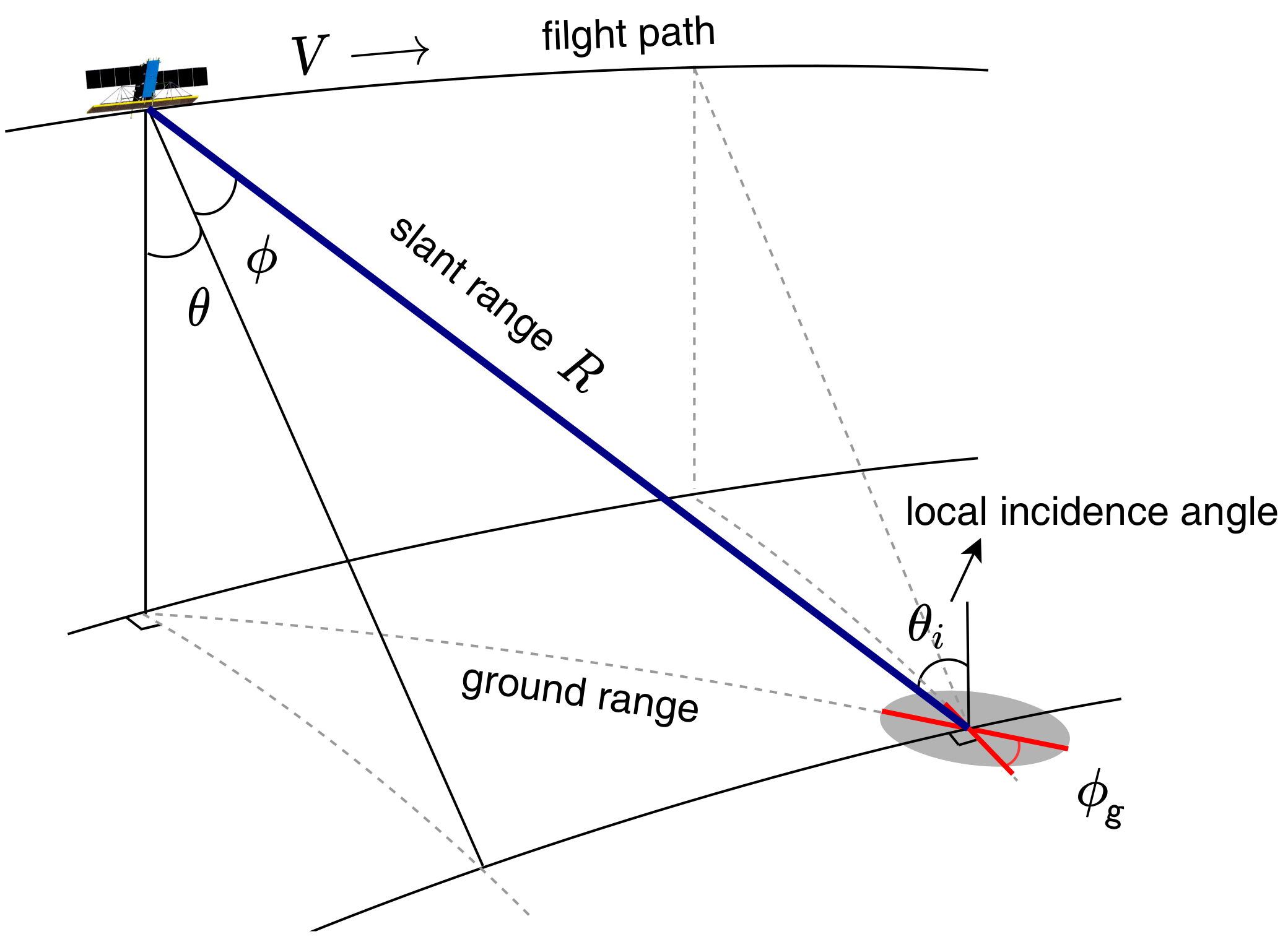
The imaging geometry is shown in Figure 2. The vector is the platform velocity relative to the ground scatterer, including the effect of Earth’s rotation, so that it is perpendicular to the zero-Doppler plane. The slant range vector and the velocity vector form the slant-range plane. The direction from radar to scatterer is measured in the two planes—the off-nadir angle in the zero-Doppler plane and the squint angle in the slant-range plane. As the SAR flies along the flight path, its antenna beam illuminates ground scatterers of interest, and the slant range distance and the squint angle vary with the relative motion. When the beam center crosses a given scatterer, the azimuth time, the slant range distance, and the squint angle are denoted by , , and , respectively.
When the slant range distance reaches its minimum, the scatterer is directly on the SAR broadside, and then the squint angle is 0 degrees. Conventional SARs observe the broadside direction, while AMAO SAR allows flexible observations in multiple squint directions. Compared with conventional SARs, the AMAO SAR has the characteristics of high geometric variations, long synthetic aperture, and time-varying radar parameters. AMAO improves the observation flexibility, acquisition efficiency, information amount, and imaging performance to a very high level; however, it also brings challenges to radiometric calibration. With the squint angle increasing, some new error sources gradually emerge; as imaging resolution increases, the synthetic aperture becomes longer and contains more variation, resulting in a complex impact on radiometric SAR measurements. Moreover, the antenna pointing is steered continuously in high-resolution imaging modes, such as (sliding) spotlight mode, so radiometric variations will accumulate over the acquisition time. These result in radiometric errors that vary highly and spatially across the swath.
2.2. Influence of AMAO on Radiometric Calibration
The radiometric calibration of SAR images is based on the SAR radar equation, which relates image intensities to well-defined physical units of the surface, usually written as [15,16,17]
where, for convenience,
is the mean power of uniform scatterer in SAR image, is the transmit power, is the antenna gain at an elevation angle , is the wavelength of the center frequency, is the system gain of the receiver, is the pulse width, is the sampling frequency of the range signal, is the pulse repetition frequency (PRF), is the range resolution, is the backscattering coefficient (normalized RCS of the surface), R is the slant range distance, is the system loss, is the local incidence angle, and is the additive noise. From Equation (1), is considered constant, so the factors of relative radiometric calibration are , R, and .
The direct use of Equation (1) is problematic for the radiometric calibration of AMAO SAR images, especially in the case of high squint and high resolution. It is not only because the conventional model does not explicitly account for the squint dependence, but also because more variations are involved within the long synthetic aperture in the squint geometry. According to literature [11,12], the squint angle of AMAO SAR may reach about 45 degrees. The higher the squint angle and the resolution, and the longer the synthetic aperture, the more relevant the variation. Therefore, the radiometric calibration model needs to be extended for AMAO space-borne SAR.
First, SAR acquisition weighting, primarily radar beam- and range-weighting, changes with the squint angle and varies spatially, especially in the high-squint high-resolution case. The AMAO SAR differs from common SARs in that the antenna beam weighting tends to be spatially variant as the squint angle increases. In the high-squint high-resolution case, even different targets within an image are applied with different antenna gain weighting, resulting in relative radiometric error within the scene. The variation in acquisition weighting between multiple observations leads to poor comparability between images. Equation (1) does not explicitly consider the antenna spatial-variant gain.
Second, the coherent integration time, which is a key parameter of the SAR system gain, changes with the observation geometry and suffers from errors due to spatial-variant acquisition weighting. Equation (1) does not account for the squint angle into the coherent integration time. According to the geometry shown in Figure 2, the coherent integration time for a given azimuth resolution can be theoretically expressed as
and the syncthetic angle
so that
where is the azimuth resolution and and are the slant range and squint angle of the beam center crossing target, respectively. It can be seen that the higher the squint angle, the longer the coherent integration time. As mentioned above, the echo signals have different acquisition weighting at different squint angles, and the weighting becomes spatially variant in the high-squint case. These will introduce errors into the coherent integration time. Thus, in the high-resolution and high-squint cases, even Equation (5) is not accurate enough from a radiometric calibration point of view.
Third, The image SNR varies with the PRF, while the PRF continuously varies in the high-squint high-resolution case [11,18,19,20], so the calibration, according to Equation (1), becomes complicated. There is an exponentially increased range cell migration arising from the high-squint geometry, so the technique of continuously varying PRF is designed to avoid collision of the receive window with the blind zone. According to the signal-to-noise ratio (SNR) equation in [16,21,22,23], SAR image SNR varies with PRF. From Equation (1), the PRF variation affects the calibration factor. Note that the dependence of the calibration factor on the PRF is based on the premise of SAR all-pass processing, and the processor gain is calibrated to keep the input and output noise power invariant. The actual SAR processing system is commonly band-pass processing in the frequency domain, and the influence of PRF needs to be analyzed in combination with the actual conditions.
Last, the SAR image brightness is affected by the relation between image resolution and the surface area, and this relationship varies with the squint angle. Equation (1) does not account for the squint dependent in the area relation. A SAR image is a two-dimensional representation of the backscattering properties of a surface, , which is the RCS normalized by area. Accurate knowledge of the surface area related to the image is important for converting the SAR image intensity into the physical unit of the normalized RCS of the surface.
3. Radar Equation for AMAO Space-Borne SAR
The radar equation for SAR is the basis for radiometric calibration. Although the common forms of the SAR radar equation have been presented in [15,16,17], new challenges arising from AMAO require careful consideration.
3.1. Relations between Target Physical Quantities and Image Response
When most of the target’s energy is focused within a single spatial resolution cell in the SAR image, the target is called a point target; otherwise, an extended target. For the point target, the image peak value depends on how good the focusing is, while the integrated energy does not because it is the weighted integral of the real-valued power (spectrum). Likewise, for natural scatterers that distribute in space randomly, the average power is independent of focusing.
For a point target, the input to the SAR system is the target RCS, , and the output is the image response. There are two methods of measuring image response: the integral method and the peak method. Reference [24] gave the relation between the two methods
where is the integrated response of the point target, is the peak of the target response, and is the area of the equivalent rectangular cell.
Gray proposed the integral method in [25], which relates the backscatter coefficient of the surface to the integrated response of the point target by
where is the integral of the image intensities of the extended target over a sufficiently large area, . The integral method has the advantage of being independent of the actual resolution and therefore more reliable, while the peak method requires exact resolution.
Rearranging Equation (7), the calibration factor is apparent
where K is the calibration factor and is the average power of the extended target over a sufficiently large area with average noise power subtracted. Thus, the integrated image response of the point target can be conveniently expressed by
With Equation (6), the peak response of the point target is
The expected RCS of the extended target within a surface resolution cell is its backscatter coefficient multiplied by the resolution cell area, written as , where is the area of the ground resolution cell. The image intensity of the extended target is then written as
There were three area symbols mentioned earlier: , , and . represents the area of the equivalent rectangular cell, represents the area of the ground resolution cell, and represents a sufficiently large ground area. Note that the ratio of and is the area projection factor, which is independent of resolution. For example, for the conventional broadside SAR image, the area of the resolution cell on the surface is written , then Equation (11) becomes . The expressions for AMAO SAR are given later in this section.
In order to calibrate the AMAO SAR images and establish the quantitative relation between the image intensity and the physical unit of the target, it is necessary to derive K and in the context of AMAO.
3.2. Calibration Factor
The calibration factor K is obtained by the integral method using the known point target. The point target signal and image response are analyzed below from the perspective of integrated energy.
3.2.1. Raw Signal Energy
As the space-borne SAR flies over and illuminates ground targets with its antenna beam, it transmits pulse signals repeatedly and receives backscattered signals. The received signal is amplitude modulated, Doppler encoded, and then focused into the high-resolution image. The phase history plays a crucial role in image focusing, but it is of no importance to the integrated response. From a radiometric point of view, the integrated response (energy) is important, so the analysis starts with the signal energy.
The energy of each transmitted pulse is the transmit power multiplied by the pulse width, , and the energy returned is determined by the radar equation. Each pulse will be compressed into an azimuth sample. The azimuth sampling interval is the pulse repetition period, . Note the azimuth variation in the pulse repetition period during squint high-resolution imaging. For an isolated point target, the energy of the raw data is the sum of all samples, written as
where is the antenna gain from the full 2-D antenna pattern, the free variable t denotes the time, in samples, and the duration from the start to stop is the azimuth coherent integration time, . Factors out of the summation are considered constant during the target exposure time.
Ideally, the integration of the radar acquisition weighting (including beam- and range-weighting) over target exposure time results in . However, the result will be affected by the variation in the acquisition weighting and pulse repetition period, leading to a deviation from the ideal
Factor D can be considered as the variation due to radar acquisition weighting.
3.2.2. SAR Processor Gain
The SAR processor performs 2-D matched filtering based on range-azimuth decoupling to output high-resolution SAR images. The processor gain is usually written as [15,16,17]
where n is the total number of integrated samples and and are the number of samples in range and azimuth, respectively. After normalizing the noise power gain, the signal power gain is n, as in Equation (1). The gain contains the PRF, which is usually constant but varies continuously at high squint and high resolution. It is sound under the premise of SAR all-pass processing. However, SAR processors are usually bandpass systems, so the gain needs to be analyzed for the actual processor.
Space-borne SARs usually use the frequency-domain processor, whose power gain to the signal peak is usually written as
where and are the bandwidth and and are the chirp rate, in range and azimuth, respectively. Note that Equation (16) gives the gain of the signal peak, in which the azimuth processing gain varies with the slant range R and along the azimuth in the high-resolution sliding spotlight case.
Due to different reference functions applied, the gain from Equation (15) is related to the sampling rate and PRF, while (16) is related to bandwidth. The frequency-domain processor is more common in space-borne SAR, so the analysis in this paper is based on the frequency-domain processor.
This paper starts with the integrated energy, focusing on the energy gain between the input and output of the processor. According to the integral method, the processor gain for an isolated target is the ratio of the integrated response to the input signal energy. For convenience and clarity, the analysis begins with the 1-D range compression and then extends to the 2-D focusing.
The range signal output by a convolution filter is
where ⊗ represents convolution.
According to the convolution theorem, it can be written in the frequency domain as
where is the range frequency.
The integrated response is pertinent to radiometric calibration, given by
The integration interval means including enough sidelobes.
According to Parseval’s theorem,
The integrated response depends on , which is a known function generated from the signal parameters, usually written as [21]
where is the bandwidth of the transmitted signal. Substituting Equation (21) into (20), the integrated response becomes
The integrated response is the energy of the input range signal, calculated in the frequency domain.
The processor gain analysis is then extended from the 1-D case to the 2-D case.
where is the output of the processor, is the input raw signal, and is the azimuth frequency. As in the 1-D case, is an amplitude-normalized band-pass filter in the frequency domain so that
where is the bandwidth for azimuth processing.
In short, the frequency-domain processor, which is an amplitude-normalized band-pass filter given by [21], maintains the input and output energies equal. From the point of view of integral method, the processor gain is equal to one. Various functions applied to the processor affect its gain and should be precisely calibrated to maintain radiometric accuracy.
3.2.3. Integrated Response and Calibration Factor
From Equation (24), the integrated energy of the processor output is equal to the energy of the raw signal, which is derived in the frequency domain and, according to Parseval’s theorem, also applies to the time-domain signal energy. The image response of a point target needs to be measured in the spatial domain. The conversion from time-domain coordinates to spatial domain coordinates uses coefficients of V for azimuth and for range. Therefore, the integrated image response is written
with Equations (14) and (24),
According to the integral method, the calibration factor is
In Equation (27), parameters for relative radiometric calibration are antenna gain pattern , slant range R, variation due to radar acquisition weighting D, and coherent integration time .
3.3. Area Projection
The RCS is pertinent to the point target, and the normalized RCS is appropriate for the extended target. The SAR radar equation for point targets has considered the equivalent rectangular resolution cell, not the physically meaningful area unit. The physical unit of the extended target is usually the backscattering coefficient, , which is the RCS normalized by surface area. Obviously, the surface area must be known for the radiometric calibration of extended targets.
From another point of view, for an isolated point target, the fact that there is only one point target in the resolution cell does not change whether the resolution cell is rectangular or skewed. However, for an extended target, many scattering elements are randomly distributed inside it. The size of the resolution cell determines the number of scattering elements contained in it, which in turn affects the image response intensity. Therefore, the physically meaningful area of the resolution cell is important for radiometric measurements of extended targets.
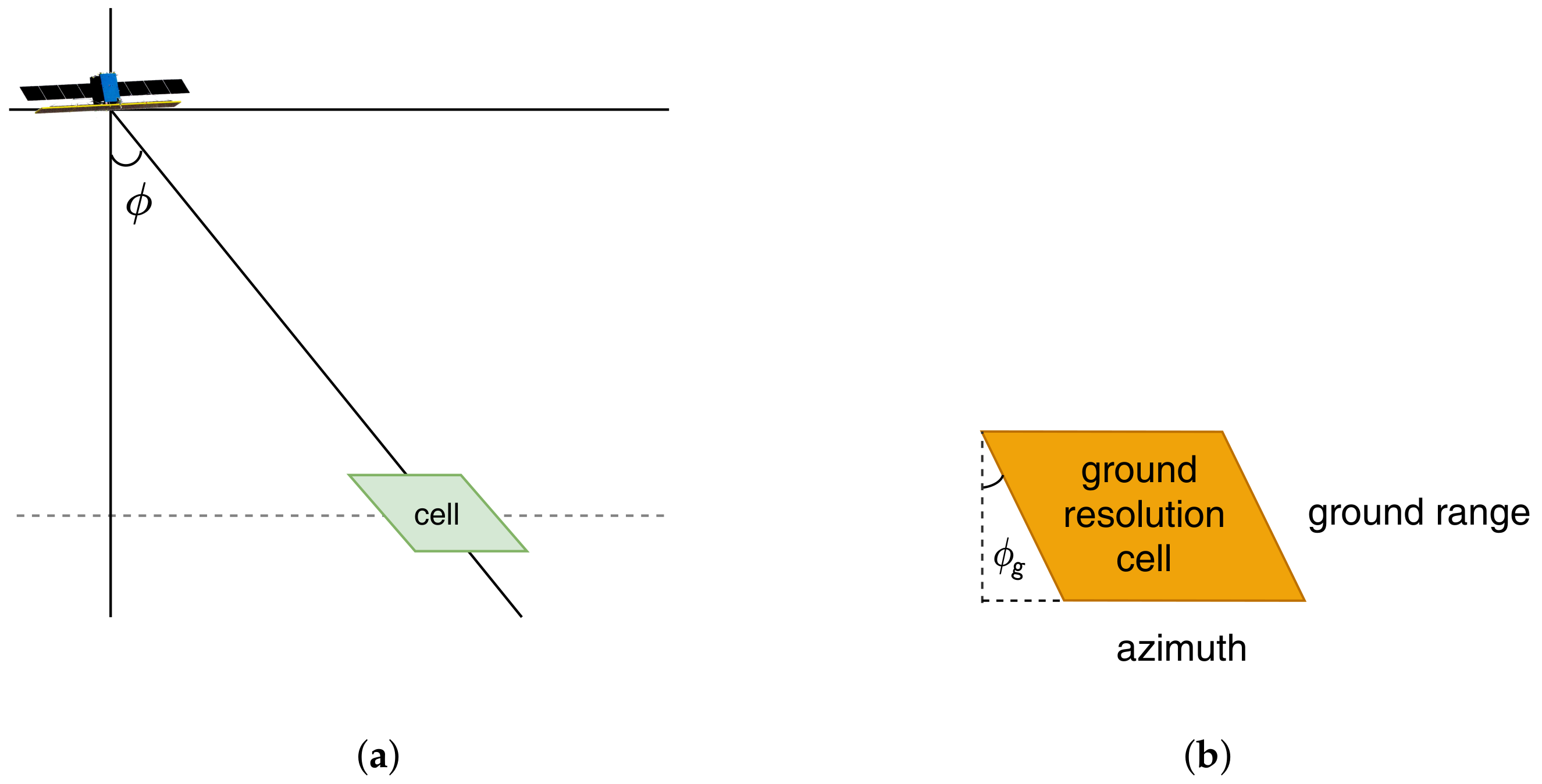
In the AMAO imaging geometry (see Figure 2), as the squint angle increases, the azimuth and slant range coordinates becomes non-orthogonal, so the resolution cell in the slant-range plane is not rectangular but skewed, as shown in Figure 3a. The same goes for the ground-range resolution cell: see Figure 3b. Angle is the angle of the ground-range direction from the cross-track direction. The ground range is expressed as , where and represent ground-range and slant-range resolutions, respectively. To calculate the area of the skewed resolution cell, it is also necessary to multiply by a factor . Therefore, the area projection factor can be written as
3.4. Radar Equation for AMAO SAR
It can be seen that Equation (29) is independent of the resolution, which comes from the advantage of the integral method. Note that compared to Equation (1), Equation (29) has three more variables that need to be corrected—D, , and , and that these parameters vary in two dimensions, especially in the high-squint high-resolution case.
4. Radiometric Normalization for AMAO Space-Borne SAR
Radiometric calibration converts intensity values of the SAR image from a qualitative representation to a quantitative representation in a physical unit. The calibration model is obtained by reformulating the SAR radar equation.
The conventional model of radiometric normalization can be obtained by reformulating Equation (1), written as
Radiometric normalization can be done by correcting , R, , and , which are corrections for antenna pattern, range spreading loss, calibration constant, and incidence angle, respectively.
An improved model of radiometric normalization can be obtained by reformulating Equation (29), written as
where, for convenience, parameters that are considered as constants are contained in
represents the average power of the extended target with average noise power subtracted so that . From Equation (31), parameters for relative calibration include antenna gain pattern , slant range R, variation due to radar acquisition weighting D, coherent integration time , local incidence angle , and the skew angle of ground range direction. As mentioned, factors D, , and vary in two dimensions. After the correction of parameters , , D, , , and , SAR images can be radiometrically normalized.
4.1. Normalization of Acquisition Weighting
Radar acquisition weighting includes beam- and range-weighting, involving three parameters: , R, and D, where D is a newly proposed parameter.
Factor D represents the relative radiometric deviation due to the azimuth variation in radar acquisition weighting. In the context of high-resolution AMAO space-borne SAR, D is range-dependent and becomes a spatial-variant as the squint angle increases. A direct way to normalize the effect of D is to perform a numerical evaluation for each resolution cell or a coarser grid, using Equation (13) and the full 2-D antenna pattern. This approach is practical for radiometric normalization but has disadvantages: point-by-point integration requires high computational cost and cannot compensate for signal weighting.
The azimuth signal magnitude can be conveniently expressed as
where A is a magnitude coefficient. The radar acquisition weighting in magnitude is written as
where is the azimuth antenna pattern. In Equation (34), only varies steeply, while and R vary gradually in azimuth. Based on this fact, Taylor expands the gradually changing part
with
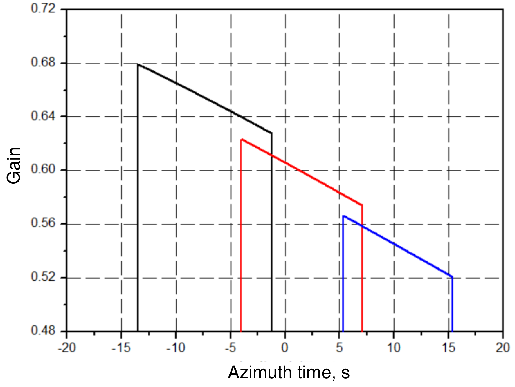
where is an elevation-dependent linear coefficient and summarizes terms of order 2 and higher. Note that is tiny, because varies so slowly in azimuth that it is approximately linear, as shown in Figure 4.
Equation (37) shows that, except for the azimuth antenna pattern, the signal weighting changes approximately linearly in azimuth.
According to Equation (37), the relative variation in can be removed from the range-compressed azimuth signal by
where is the reference squint angle, usually the squint angle at which the beam center crosses the scene center. Note that has been ignored at this point since varies slowly in azimuth.
The advantage of linear correction is that it is not insensitive to errors in antenna pointing and Doppler estimation, so this method is recommended. However, as the azimuth length of the scene increases, the simple linear model is insufficient to characterize the azimuth variation of the antenna gain. Possible residual errors can be easily corrected after image formation.
In short, relative variations in acquisition weighting can be normalized through a linear model given by Equation (38), thereby D normalized, along with the antenna pattern and the slant range R. This approach is insensitive to errors in antenna pointing and Doppler estimation.
4.2. Normalization of Coherent Integration Time
The coherent integration time, , is a variable in Equation (31). It is usually calculated by the theoretical expression provided in Equation (5). However, the resolution at different locations in the scene will vary somewhat in the sliding spotlight image, with the maximum deviation appearing between the center and edges, leading to a complicated calculation of . Meanwhile, the direct use of the expression will introduce errors due to model approximation, especially in the high-squint case. A more accurate approach is to calculate directly from the time-frequency relation
where and are the start and end of the azimuth integration frequency.
4.3. Correction of Area Projection Factor
At this point, variables in Equation (31), including , , D, and , are removed, with and remaining. The factor is the area projection factor from the surface resolution cell to the equivalent rectangular cell. With the positions of the platform and ground points, and can be directly and precisely calculated and then normalized.
5. Simulation Experiments
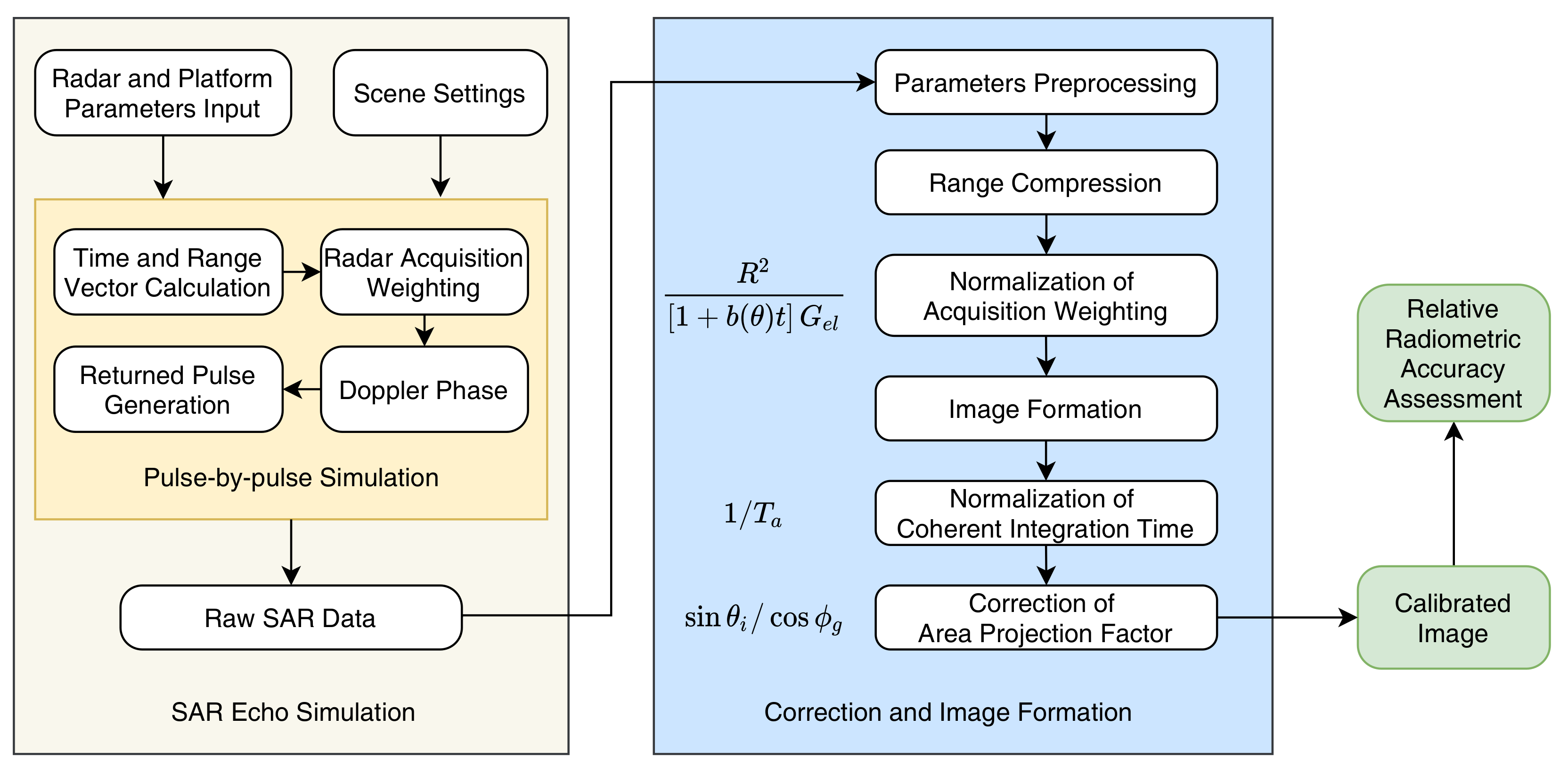
Experiments are conducted in this section to verify the proposed models. First, the echo signals are generated by simulating the real physical processes of SAR acquisition, with parameters listed in Table 1. The echoes are then focused into images with a carefully designed and precisely calibrated processor, using the models presented in Section 4. Finally, radiometric accuracy is evaluated to verify the proposed models. The block diagram of the simulation flow is shown in Figure 5.
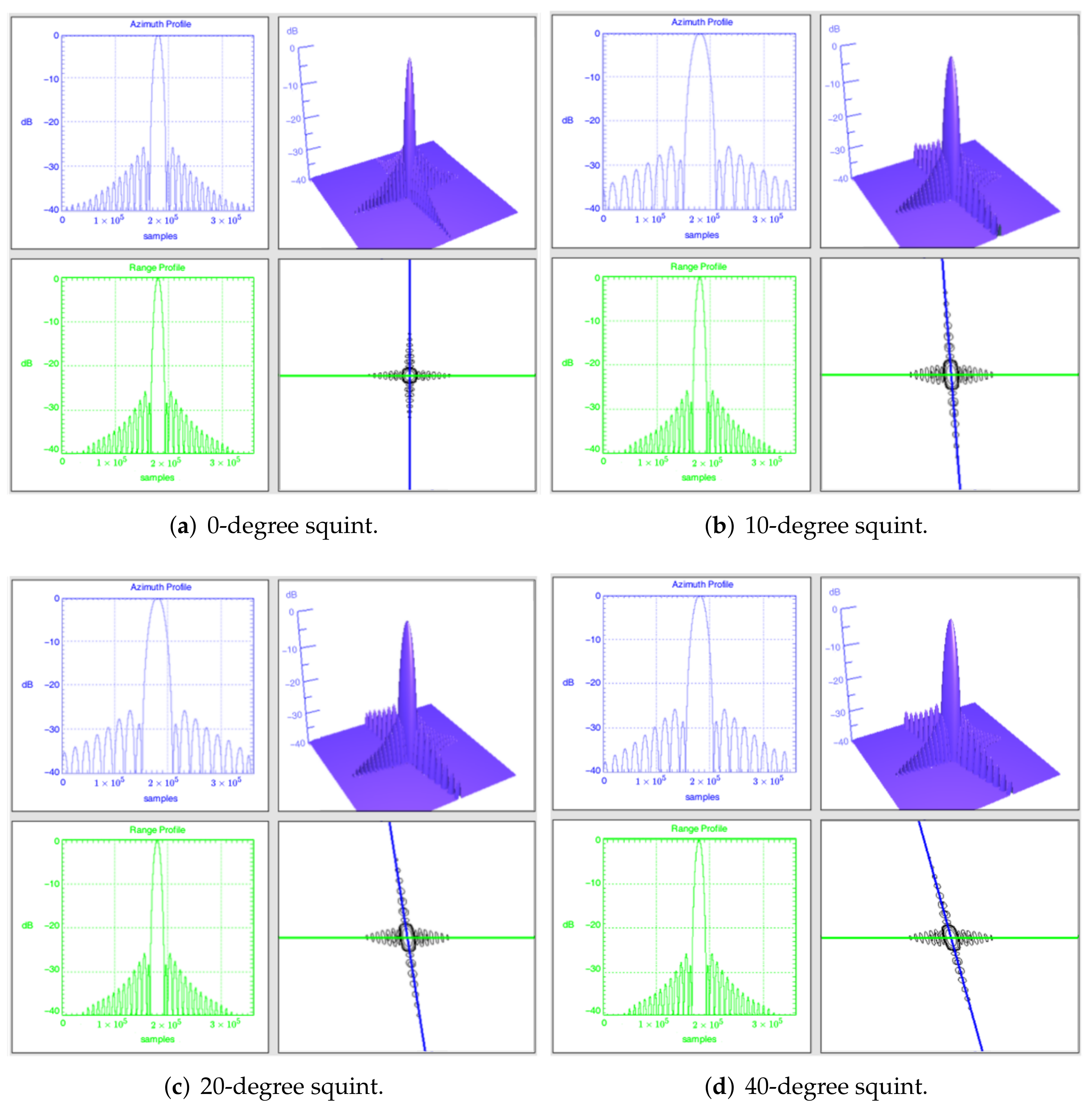
First, point targets are set at the scene center, imaged with different squint angles from 0 to 40 degrees in 5-degree steps. Partial imaging results are shown in Figure 6. The integrated responses of point targets are measured in calibrated images, and the results are listed in Table 2. Results show that the relative radiometric deviation is about 0.024 dB (peak-to-peak), indicating the excellent performance of the proposed method.
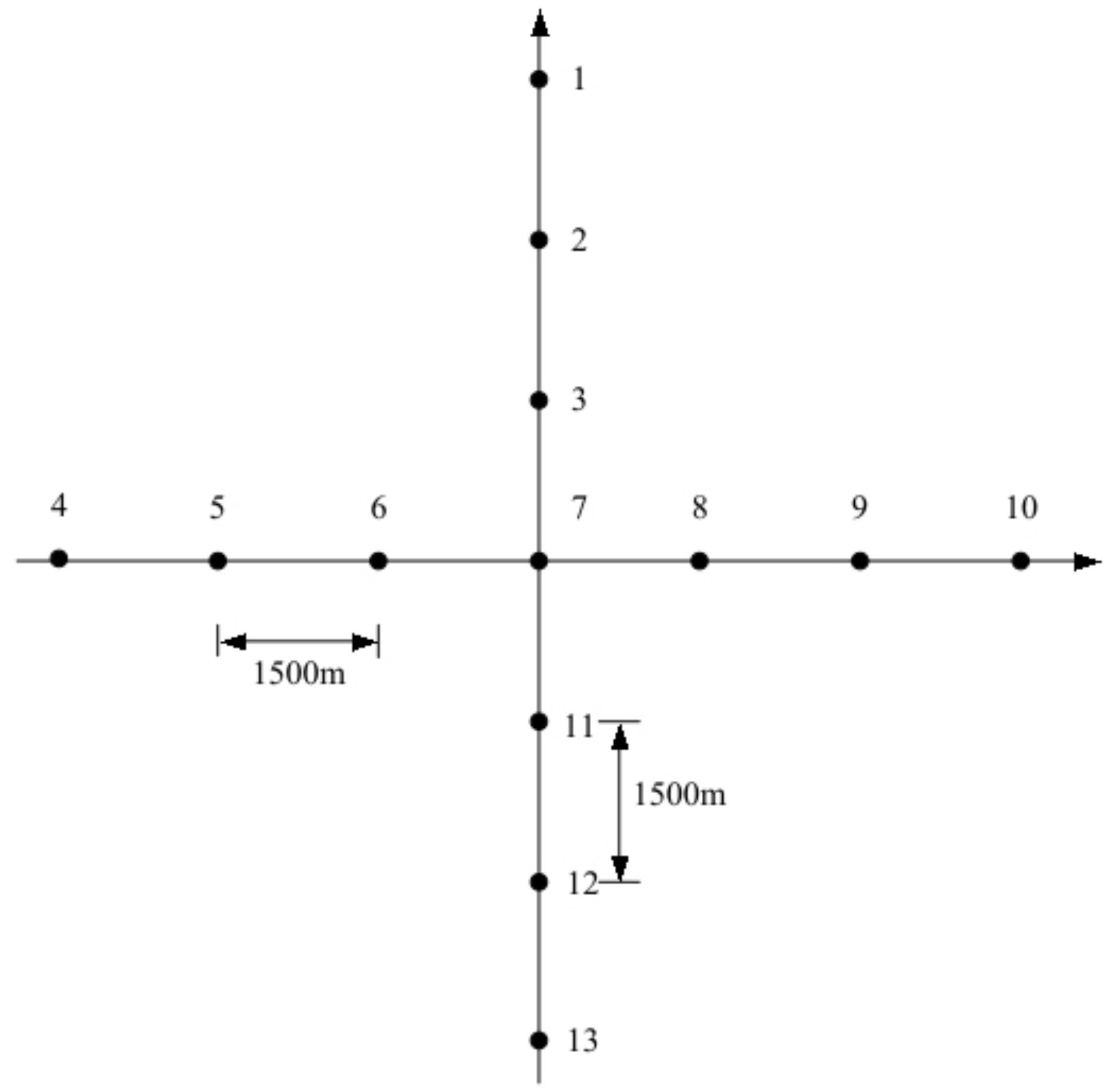
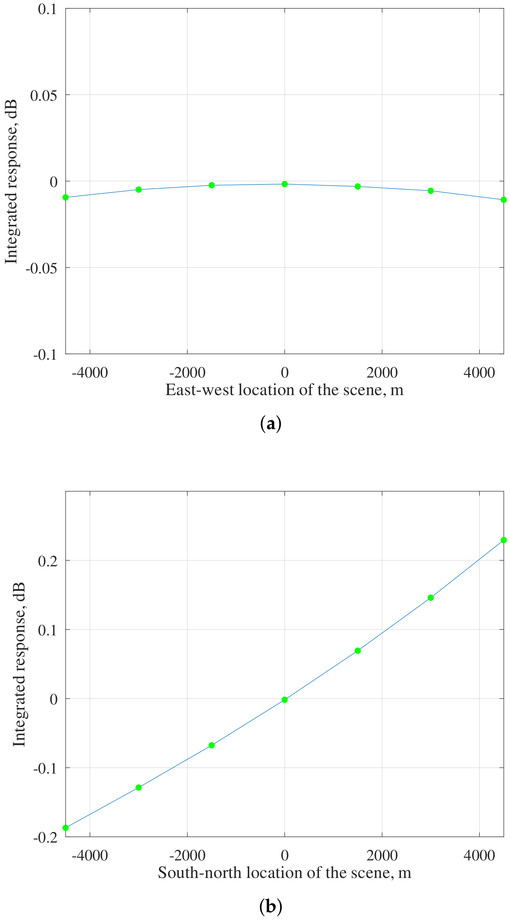
Next, point targets are distributed across the scene in a cross-shaped array with 1500 m east-west and north-south spacing, as shown in Figure 7. The scene is imaged with a nominal squint angle of 40 degrees. After image formation and radiometric normalization, the integrated response of each target is measured. All measurements are plotted in Figure 8.
Figure 8a shows the results for targets 4 to 10, which are set along the east-west direction. Results show a tiny deviation of about 0.01 dB (peak-to-peak). According to the orbital parameter settings, targets 4 to 10 are roughly distributed along the cross-track direction, thus indicating the proposed method with good performance in the range direction. Figure 8b shows the results for targets 1 to 3 and 11 to 13, which are set along the south-north direction. Results show that the proposed method reduces the azimuth radiometric variation to about ±0.2 dB. The residual error increases with the azimuth length of the scene. As mentioned in Section 4.1, although most of the azimuth variation in antenna gain can be corrected using the linear model, it is not sufficient in the case of high-resolution sliding spotlight mode. After the complementary correction of antenna gain, the relative radiometric deviation is further reduced to about 0.1 dB.
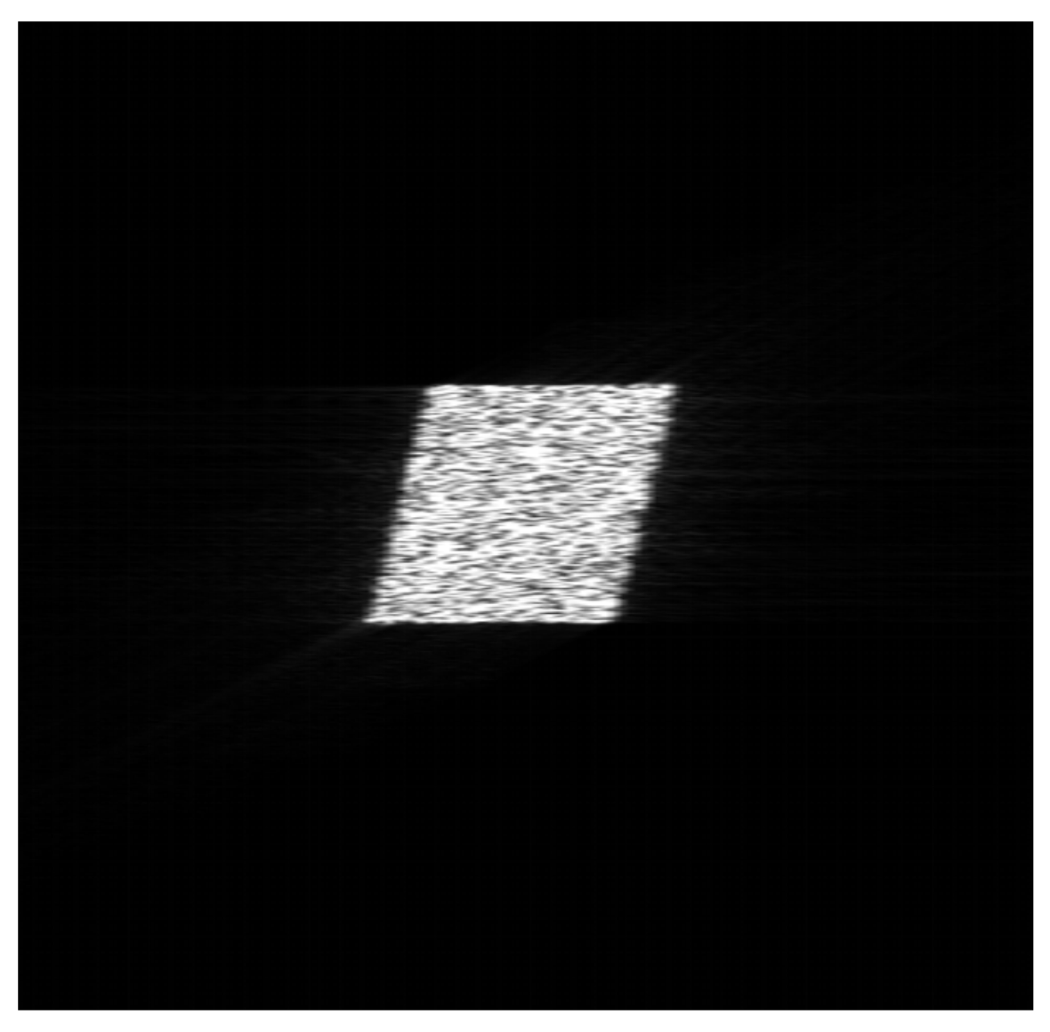
Finally, an extended target simulation is carried out. The target size is 20 m × 20 m, containing massive scattering elements spaced 0.02 m apart. The RCS of each scattering element is set to one. The squint angle is set to 40 degrees. Figure 9 shows the imaging result. The average power of the extended target image is measured, and the result is 346.564. In order to absolutely verify the calibration accuracy, the number of scattering elements contained in the resolution cell is carefully calculated, and the result is 341.786. The measured value is very close to the theoretically calculated value, with a deviation of about 1.4%, and the decibel form is 0.06 dB.
6. Discussion
6.1. Discussion on SAR Radar Equation for AMAO Space-Borne SAR
This paper derived a form of radar equation in the context of AMAO SAR (see Equation (29)). For a convenient comparison with the common form of SAR radar equation (see Equation (1)), the two equations are rearranged and written as follows
Equation (40) comes from Equation (1), and Equation (41) from Equation (29), and the two can be compared item by item. From left to right, the first factor is considered constant and is the same in both equations. The second factor represents radar acquisition weighting. The proposed model takes into account the squint geometry and the spatial variant in weighting. The third factor represents the coherent integration time for range and azimuth. The fourth factor is a coefficient, which depends on PRF and resolution in the conventional model, but is independent of them in the proposed model. The fifth factor represents the area projection, and the new model accounts for the non-orthogonality of the 2-D resolution directions. Equation (41) does not contain the factor because represents the average power of the extended target with average noise power subtracted.
From Equations (40) and (41), the proposed radar equation in the context of AMAO SAR takes into account the following points.
- 1.
- The antenna pattern becomes spatially variant with increasing squint angle and resolution. Targets at different locations in the scene are exposed to different antenna patterns, each of which is a different cut of the 2-D pattern of the squint beam, resulting in a complex 2-D effect on the image. Therefore, the factor D is defined to account for this effect.
- 2.
- Factors in Equation (40) represent the synthetic time without squint. The expression containing the squint angle is given by Equation (5). However, errors arise even from the model of (5) in the squint case. Meanwhile, the resolution at different locations in the scene will vary somewhat in the sliding spotlight image, with the maximum deviation appearing between the center and edges, leading to a complicated but not accurate calculation of . An accurate approach is to calculate directly, so is included in the proposed model.
- 3.
- AMAO space-borne SAR will utilize the continuously varying PRF technique to compensate ultra-large range cell migration. The conventional model needs to account for PRF variation, as PRF is contained in Equation (1). On the other hand, the frequency-domain processor is commonly used for space-borne SARs, and its power gain to the signal peak is written as , which is independent of PRF. From a calibration point of view, signal energy gain is more important than peak gain. Therefore, this paper derives the processor gain based on the integration method, and the obtained gain to energy is equal to one. Therefore, the PRF variation need not be contained in the radiometric calibration model.
- 4.
- The derivation of calibration model in this paper is based on the integral method, which has the advantage of being resolution independent. Benefiting from this, the proposed model is also independent of resolution and thus more reliable.
- 5.
- A new factor is introduced, , to account for non-orthogonal coordinates and the skewed resolution cells. The number of scattering elements decreases as the resolution cell is skewed, causing radiometric attenuation in the image.
6.2. Discussion on Calibration Model with Experimental Results
The experimental results verified the proposed calibration model and method. Results for different squint angles of 0–40 degrees, as well as the results for the range direction within the scene, are reduced to a negligible level.
As mentioned in Section 4.1, based on the fact that the acquisition weighting changes slowly in azimuth, this paper recommends a linear model for normalization. Meanwhile, it is also mentioned that, for very-high-resolution and very-high-squint SAR images, there will be residual errors in the whole swath because the linear model is not accurate enough. Even so, since it is not affected by errors in antenna pointing and Doppler center estimation, the linear model can still be used, and it is not difficult to compensate for the residual errors in the focused image. As shown in Figure 8, a relative deviation of about 0.4 dB (peak-to-peak) across the whole scene arises and is then compensated by post-processing calibration.
The effect of the skewed resolution cell is a new problem arising from the high squint angle. This effect is verified by the extended target simulation, where the experimental result is in good agreement with the value calculated through the proposed model.
7. Conclusions
Accurate and consistent radiometric measurements are the basis for quantitative applications of SAR image products. AMAO space-borne SAR improves the flexibility of data acquisition, while bringing challenges to radiometric calibration. The larger the squint angle, the higher the resolution, and the more the variations involved, leading to more difficulty in achieving accurate radiometric measurements. However, radiometric accuracy is a system demand that should be and needs to be achieved through improved models and innovative methods.
This paper addressed the new issues in radiometric calibration arising from the AMAO space-borne SAR system. An appropriate form of the SAR radar equation is derived for AMAO space-borne SAR. Benefiting from the use of the integration method, the proposed model has the advantage of being PRF- and resolution-independent. Meanwhile, special issues are accounted for AMAO calibration, such as the spatial-variant acquisition weighting and the area projection factor for skewed resolution cells. On these bases, the calibration model is obtained by reformulating the novel AMAO SAR equation, and the corresponding normalization method is then proposed. The good experimental performance indicators verify the correctness of proposed models and the effectiveness of the correction method.
Author Contributions
Conceptualization, J.C. and J.H.; methodology, J.H. and P.W.; software, P.W.; validation, J.H. and Y.G.; formal analysis, J.H.; investigation, J.H.; resources, P.W.; data curation, Y.G.; writing—original draft preparation, J.H. and Y.G.; writing—review and editing, J.H., J.C. and P.W.; visualization, P.W. and Y.G.; supervision, J.C.; project administration, P.W.; funding acquisition, P.W. All authors have read and agreed to the published version of the manuscript.
Funding
This research received no external funding.
Institutional Review Board Statement
Not applicable.
Informed Consent Statement
Not applicable.
Data Availability Statement
Not applicable.
Acknowledgments
The authors would like to express their gratitude to the anonymous reviewers and the associate editor for their constructive comments on the paper.
Conflicts of Interest
The authors declare no conflict of interest.
Abbreviations
The following abbreviations are used in this manuscript:
| AMAO | Azimuthal multi-angle observation |
| RCS | radar cross section |
| SAR | Synthetic aperture radar |
| 2-D | Two-dimensional |
References
- Kraus, T.; Ribeiro, J.P.T.; Bachmann, M.; Steinbrecher, U.; Grigorov, C. Concurrent Imaging for TerraSAR-X: Wide-Area Imaging paired with High-Resolution Capabilities. IEEE Trans. Geosci. Remote Sens. 2022, 60, 5220314. [Google Scholar] [CrossRef]
- Franceschetti, G.; Guida, R.; Iodice, A.; Riccio, D.; Ruello, G. Efficient Simulation of hybrid stripmap/spotlight SAR raw signals from extended scenes. IEEE Trans. Geosci. Remote Sens. 2004, 42, 2385–2396. [Google Scholar] [CrossRef]
- Mittermayer, J.; Wollstadt, S.; Prats-Iraola, P.; Scheiber, R. The TerraSAR-X Staring Spotlight Mode Concept. IEEE Trans. Geosci. Remote Sens. 2014, 52, 3695–3706. [Google Scholar] [CrossRef]
- Mittermayer, J.; Kraus, T.; López-Dekker, P.; Prats-Iraola, P.; Krieger, G.; Moreira, A. Wrapped Staring Spotlight SAR. IEEE Trans. Geosci. Remote Sens. 2016, 54, 5745–5764. [Google Scholar] [CrossRef]
- Meta, A.; Mittermayer, J.; Steinbrecher, U.; Prats, P. Investigations on the TOPSAR acquisition mode with TerraSAR-X. In Proceedings of the 2007 IEEE International Geoscience and Remote Sensing Symposium, Barcelona, Spain, 23–27 July 2007; pp. 152–155. [Google Scholar] [CrossRef]
- Mittermayer, J.; Wollstadt, S.; Prats-Iraola, P.; Lopez-Dekker, P.; Krieger, G.; Moreira, A. Bidirectional SAR Imaging Mode. IEEE Trans. Geosci. Remote Sens. 2013, 51, 601–614. [Google Scholar] [CrossRef] [Green Version]
- Chen, J.; Yang, W.; Wang, P.; Zeng, H.; Men, Z.; Li, C. Review of Novel Azimuthal Multi-angle Observation Space-borne SAR Technique. J. Radars 2020, 9, 205–220. [Google Scholar] [CrossRef]
- Yang, W.; Ma, X. A Novel Spaceborne SAR Imaging Mode for Moving Target Velocity Estimation. In Proceedings of the 2016 International Conference on Control, Automation and Information Sciences (ICCAIS), Ansan, Korea, 27–29 October 2016; pp. 13–16. [Google Scholar] [CrossRef]
- Wang, Y.; Yang, W.; Chen, J.; Kuang, H.; Liu, W.; Li, C. Azimuth Sidelobes Suppression Using Multi-Azimuth Angle Synthetic Aperture Radar Images. Sensors 2019, 19, 2764. [Google Scholar] [CrossRef] [PubMed] [Green Version]
- Huang, J.; Wang, P.; Chen, J. Impact of 2-D Antenna Pattern on Radiometric Calibration of Azimuthal Multi-angle Observation Spaceborne SAR. In Proceedings of the 2021 Photonics Electromagnetics Research Symposium (PIERS), Hangzhou, China, 21–25 November 2021; pp. 2835–2839. [Google Scholar] [CrossRef]
- Men, Z.; Wang, P.; Li, C.; Chen, J.; Liu, W.; Fang, Y. High-Temporal-Resolution High-Spatial-Resolution Spaceborne SAR Based on Continuously Varying PRF. Sensors 2017, 17, 1700. [Google Scholar] [CrossRef] [PubMed] [Green Version]
- Kuang, H.; Wang, T.; Gao, H.; Yu, H.; Liu, L.; Zhang, R. Geometry and Signal Properties of Multiple Azimuth Angle Spaceborne SAR. In Proceedings of the IET International Radar Conference (IET IRC 2020), Online Conference, 4–6 November 2020; pp. 379–383. [Google Scholar] [CrossRef]
- Ansari, H.; De Zan, F.; Parizzi, A.; Eineder, M.; Goel, K.; Adam, N. Measuring 3-D Surface Motion with Future SAR Systems Based on Reflector Antennae. IEEE Geosci. Remote Sens. Lett. 2016, 13, 272–276. [Google Scholar] [CrossRef] [Green Version]
- Jung, H.S.; Lu, Z.; Shepherd, A.; Wright, T. Simulation of the SuperSAR Multi-Azimuth Synthetic Aperture Radar Imaging System for Precise Measurement of Three-Dimensional Earth Surface Displacement. IEEE Trans. Geosci. Remote Sens. 2015, 53, 6196–6206. [Google Scholar] [CrossRef]
- Curlander, J.C.; McDonough, R.N. Synthetic Aperture Radar: Systems and Signal Processing; John Wiley & Sons: Hoboken, NJ, USA, 1991. [Google Scholar]
- Freeman, A.; Curlander, J.C. Radiometric Correction and Calibration of SAR Images. Photogramm. Eng. Remote Sens. 1989, 55, 1295–1301. [Google Scholar]
- Shimada, M. Imaging from Space-Borne and Airborne SARs, Calibration, and Applications; CRC Press: Boca Raton, FL, USA, 2018. [Google Scholar] [CrossRef]
- Mao, Q.; Jin, G.; Ji, W.; Xu, X.; Sun, Y.; Xu, H.; Ouyang, S. Varied PRF Sequence Design Method for Space-borne UHRSL-SAR. In Proceedings of the 2020 IEEE 5th Information Technology and Mechatronics Engineering Conference (ITOEC), Chongqing, China, 12–14 June 2020; pp. 259–263. [Google Scholar] [CrossRef]
- Zeng, H.; Chen, J.; Yang, W.; Zhu, Y.; Wang, P. Image formation algorithm for highly-squint strip-map SAR onboard high-speed platform using continuous PRF variation. In Proceedings of the 2014 IEEE Geoscience and Remote Sensing Symposium, Quebec City, QC, Canada, 13–18 July 2014; pp. 1117–1120. [Google Scholar] [CrossRef]
- Zhang, Y.; Yu, Z.; Li, C. Effects of PRF variation on space-borne SAR imaging. In Proceedings of the 2013 IEEE International Geoscience and Remote Sensing Symposium—IGARSS, Melbourne, Australia, 21–26 July 2013; pp. 1336–1339. [Google Scholar] [CrossRef]
- Cumming, I.G.; Wong, F.H. Digital Processing of Synthetic Aperture Radar Data: Algorithms and Implementation; Artech House Remote Sensing Library, Artech House Inc.: Norwood, MA, USA, 2004. [Google Scholar]
- Maître, H. (Ed.) Processing of Synthetic Aperture Radar Images; ISTE Wiley: London, UK; Hoboken, NJ, USA, 2008. [Google Scholar] [CrossRef]
- El-darymli, K.; Mcguire, P.; Gill, E.; Power, D.; Moloney, C. Understanding the Significance of Radiometric Calibration for Synthetic Aperture Radar Imagery. In Proceedings of the 2014 IEEE 27th Canadian Conference on Electrical and Computer Engineering (CCECE), Toronto, ON, Canada, 4–7 May 2014; pp. 1–6. [Google Scholar] [CrossRef]
- Ulander, I.M.H. Accuracy of using point targets for SAR calibration. IEEE Trans. Aerosp. Electron. Syst. 1991, 27, 139–148. [Google Scholar] [CrossRef]
- Gray, A.L.; Vachon, P.W.; Livingstone, C.E.; Lukowski, T.I. Synthetic Aperture Radar Calibration Using Reference Reflectors. IEEE Trans. Geosci. Remote Sens. 1990, 28, 374–383. [Google Scholar] [CrossRef]
Figure 1.
Illustrations of AMAO. (a) Detailed observation of high-value targets in multi-angles, long-exposure spotlight mode; (b) Flexible observation of high-value targets in a wide area; (c) High-resolution wide-swath mode.
Figure 1.
Illustrations of AMAO. (a) Detailed observation of high-value targets in multi-angles, long-exposure spotlight mode; (b) Flexible observation of high-value targets in a wide area; (c) High-resolution wide-swath mode.

Figure 2.
AMAO SAR imaging geometry.

Figure 3.
Schematic of the skewed resolution cell. (a) Skewed resolution cell in the slant-range plane; (b) Skewed ground resolution cell.
Figure 3.
Schematic of the skewed resolution cell. (a) Skewed resolution cell in the slant-range plane; (b) Skewed ground resolution cell.

Figure 4.
Antenna gain as a function of azimuth time. The black, red and blue lines are the antenna gains of targets positioned at the start, center and end of the scene, respectively.
Figure 4.
Antenna gain as a function of azimuth time. The black, red and blue lines are the antenna gains of targets positioned at the start, center and end of the scene, respectively.

Figure 5.
Block diagram of simulation processing.

Figure 6.
Partial imaging results of point targets at different squint angles.

Figure 7.
Point target array settings.

Figure 8.
The distribution of the integrated response of targets at different locations in the scene. (a) Radiometric variation of the scene from east to west; (b) Radiometric variation of the scene from south to north.
Figure 8.
The distribution of the integrated response of targets at different locations in the scene. (a) Radiometric variation of the scene from east to west; (b) Radiometric variation of the scene from south to north.

Figure 9.
Imaging result of extended target.


Table 1.
AMAO SAR parameters.
| Parameters | Value |
|---|---|
| Wavelength | 0.03 m |
| Nominal squint angle 1 | 0–40 degrees, 5 degrees step |
| Off-nadir angle | −15 degrees |
| Nominal resolution | 0.25 in azimuth and slant-range, respectively |
| Antenna size | 4.8 m in azimuth and 2.5 m in elevation |
1 The nominal squint angle is the boresight squint angle of the scene center.
Table 2.
Integrated energy of point targets imaged with different squint angles.
| Squint angle (degree) | 0 | 5 | 10 | 15 | 20 | 25 | 30 | 35 | 40 |
| Integrated energy (dB) | −0.0249 | −0.0251 | −0.0254 | −0.0234 | −0.0224 | −0.0219 | −0.0182 | −0.0125 | −0.0017 |
Publisher’s Note: MDPI stays neutral with regard to jurisdictional claims in published maps and institutional affiliations. |
© 2022 by the authors. Licensee MDPI, Basel, Switzerland. This article is an open access article distributed under the terms and conditions of the Creative Commons Attribution (CC BY) license (https://creativecommons.org/licenses/by/4.0/).
Share and Cite
MDPI and ACS Style
Huang, J.; Chen, J.; Guo, Y.; Wang, P. Formulation of Radiometric Calibration for Azimuthal Multi-Angle Observation Space-Borne SAR. Sustainability 2022, 14, 6757. https://0-doi-org.brum.beds.ac.uk/10.3390/su14116757
AMA Style
Huang J, Chen J, Guo Y, Wang P. Formulation of Radiometric Calibration for Azimuthal Multi-Angle Observation Space-Borne SAR. Sustainability. 2022; 14(11):6757. https://0-doi-org.brum.beds.ac.uk/10.3390/su14116757
Chicago/Turabian StyleHuang, Jianjun, Jie Chen, Yanan Guo, and Pengbo Wang. 2022. "Formulation of Radiometric Calibration for Azimuthal Multi-Angle Observation Space-Borne SAR" Sustainability 14, no. 11: 6757. https://0-doi-org.brum.beds.ac.uk/10.3390/su14116757
Note that from the first issue of 2016, this journal uses article numbers instead of page numbers. See further details here.