
Micro-Siting of Wind Turbines in an Optimal Wind Farm Area Using Teaching–Learning-Based Optimization Technique

 ,
,  ,
,  ,
,  and
and 
Abstract
:1. Introduction
- Minimization of the land area of wind farm
- Maximization of the power production
- Minimization of the total cost
2. Materials and Methods
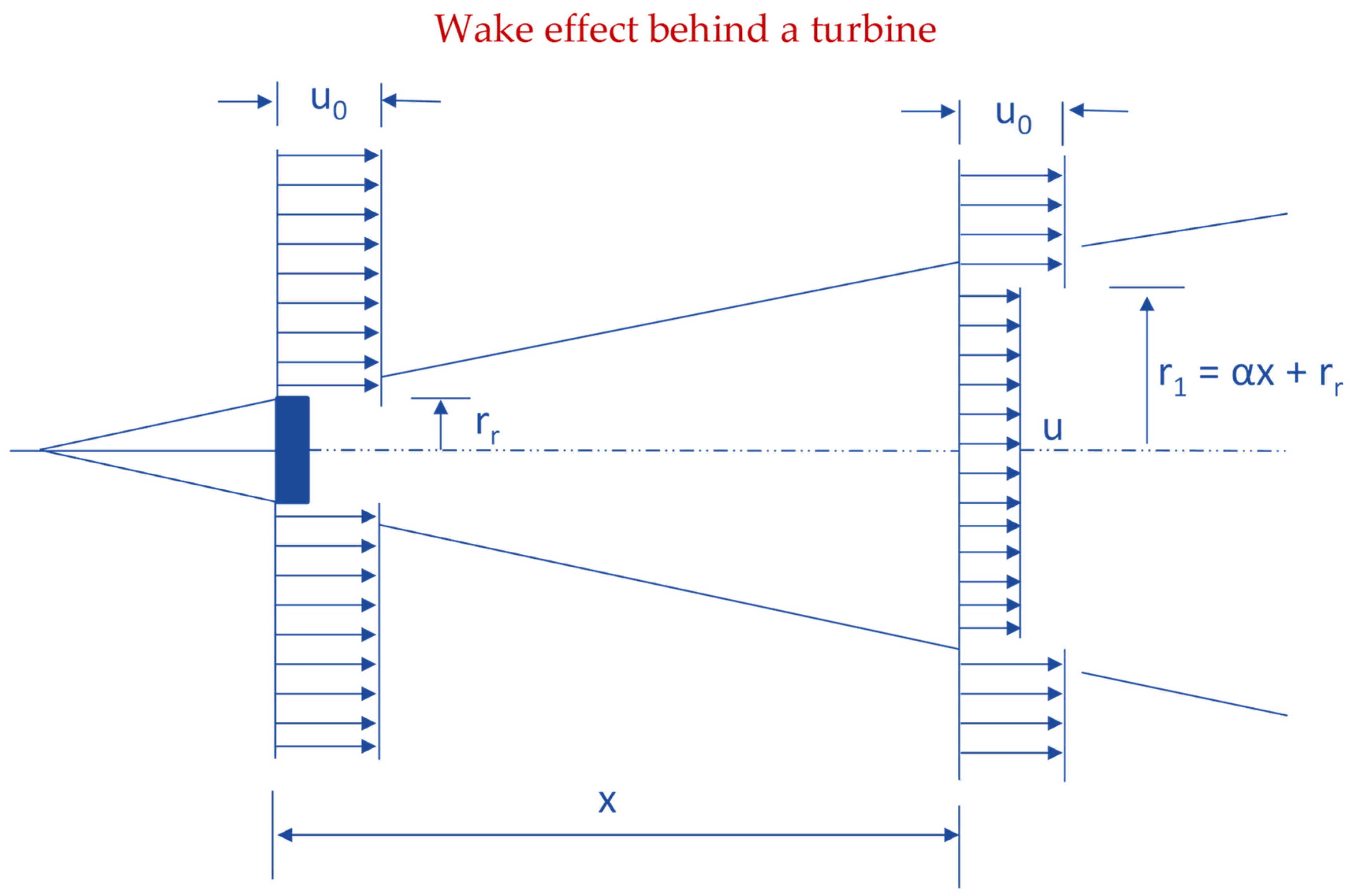
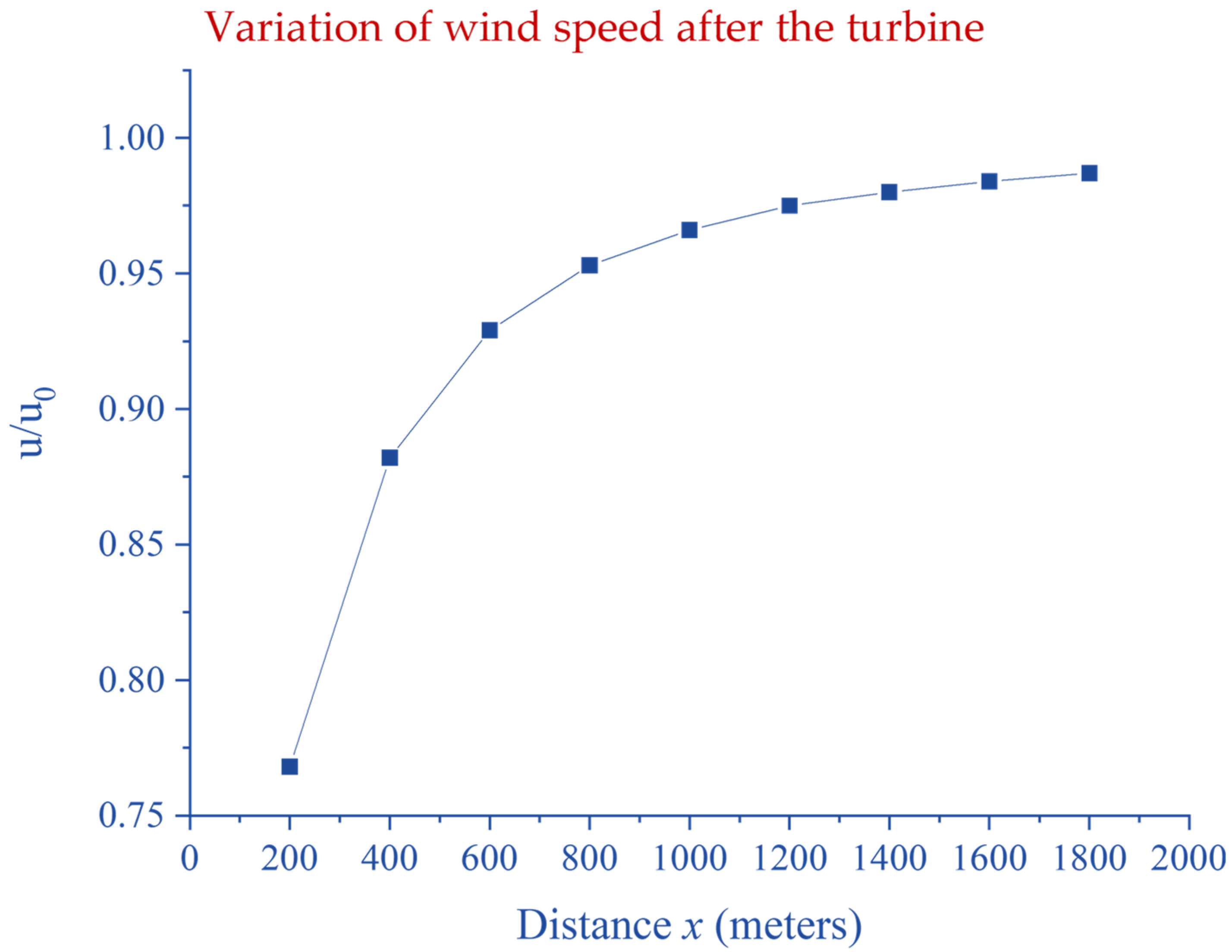
2.1. Jensen’s Wake Effect Modeling
2.2. Fitness Evaluation
2.2.1. Wind Farm Cost Estimation
2.2.2. Wind Farm Power Estimation
2.2.3. Evaluation of Fitness Function
2.2.4. Calculation of Efficiency
- .
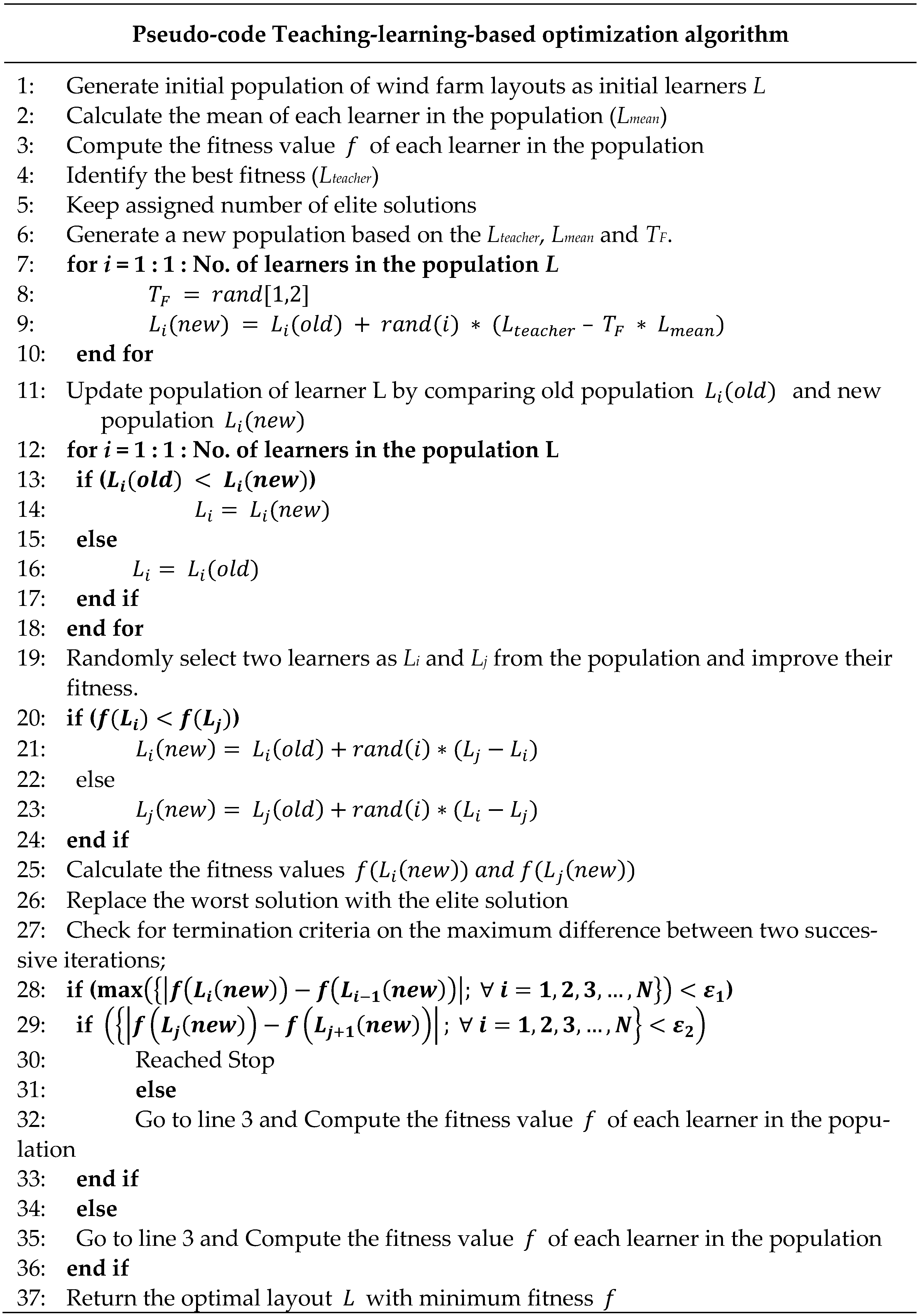
2.3. Elitist Teaching–Learning-Based Optimization Algorithm
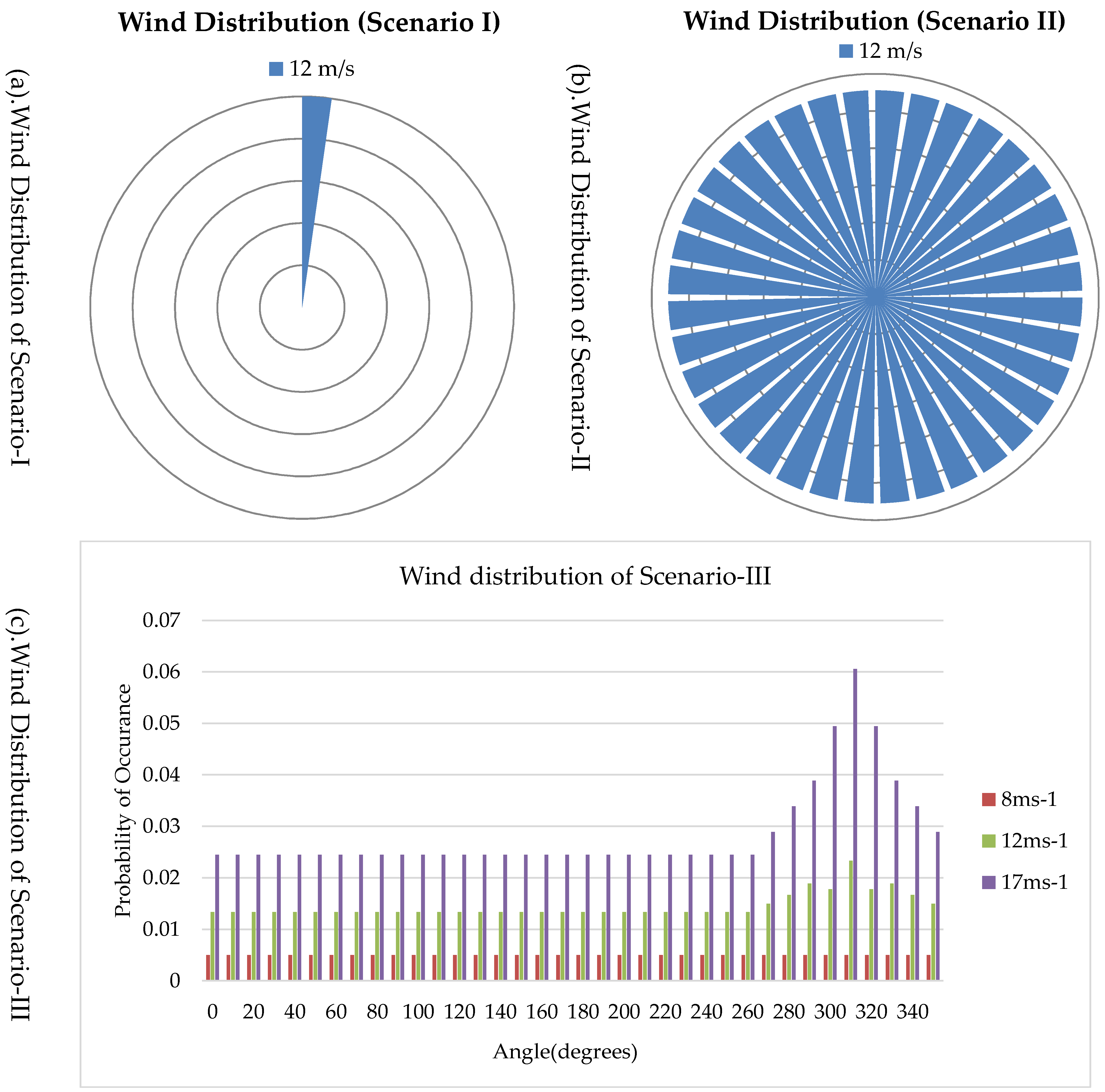
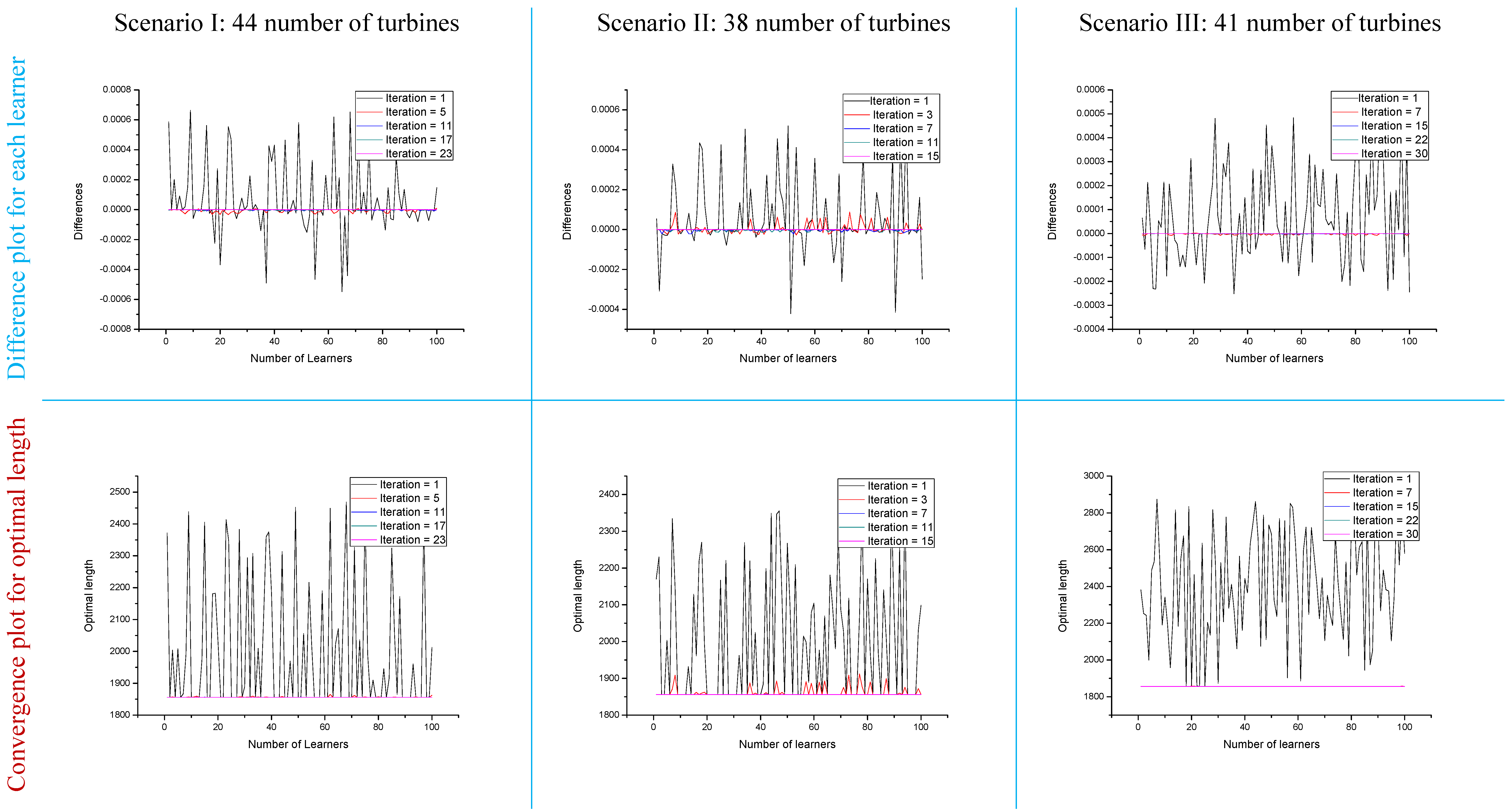
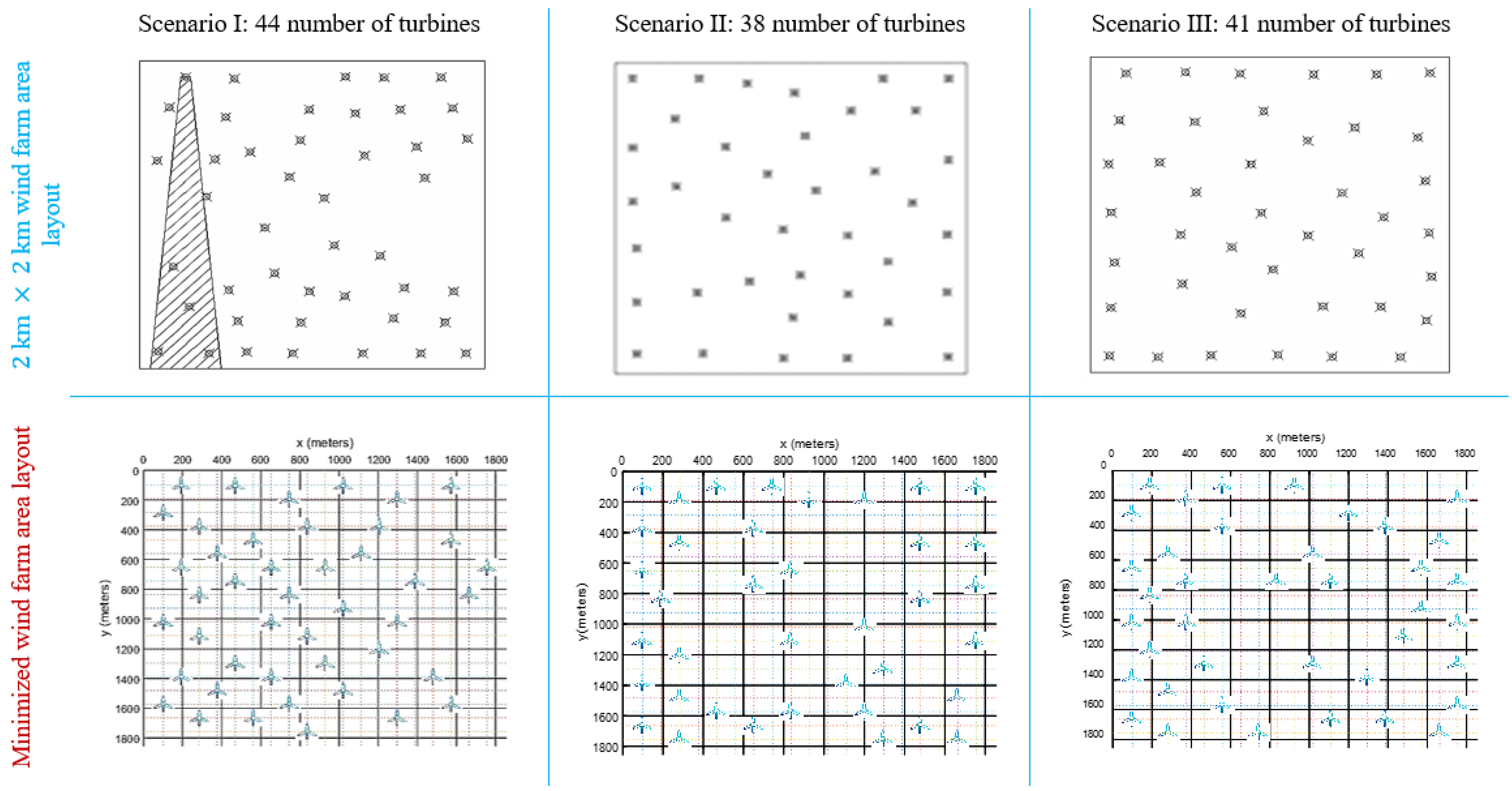
2.4. Different Wind Scenarios
2.4.1. Scenario-I: Uni-Directional Wind with the Identical Velocity
2.4.2. Scenario-II: Multi-Directional Wind with the Identical Velocity
2.4.3. Scenario-III: Multi-Directional Wind with Variable Wind Velocity
3. Results
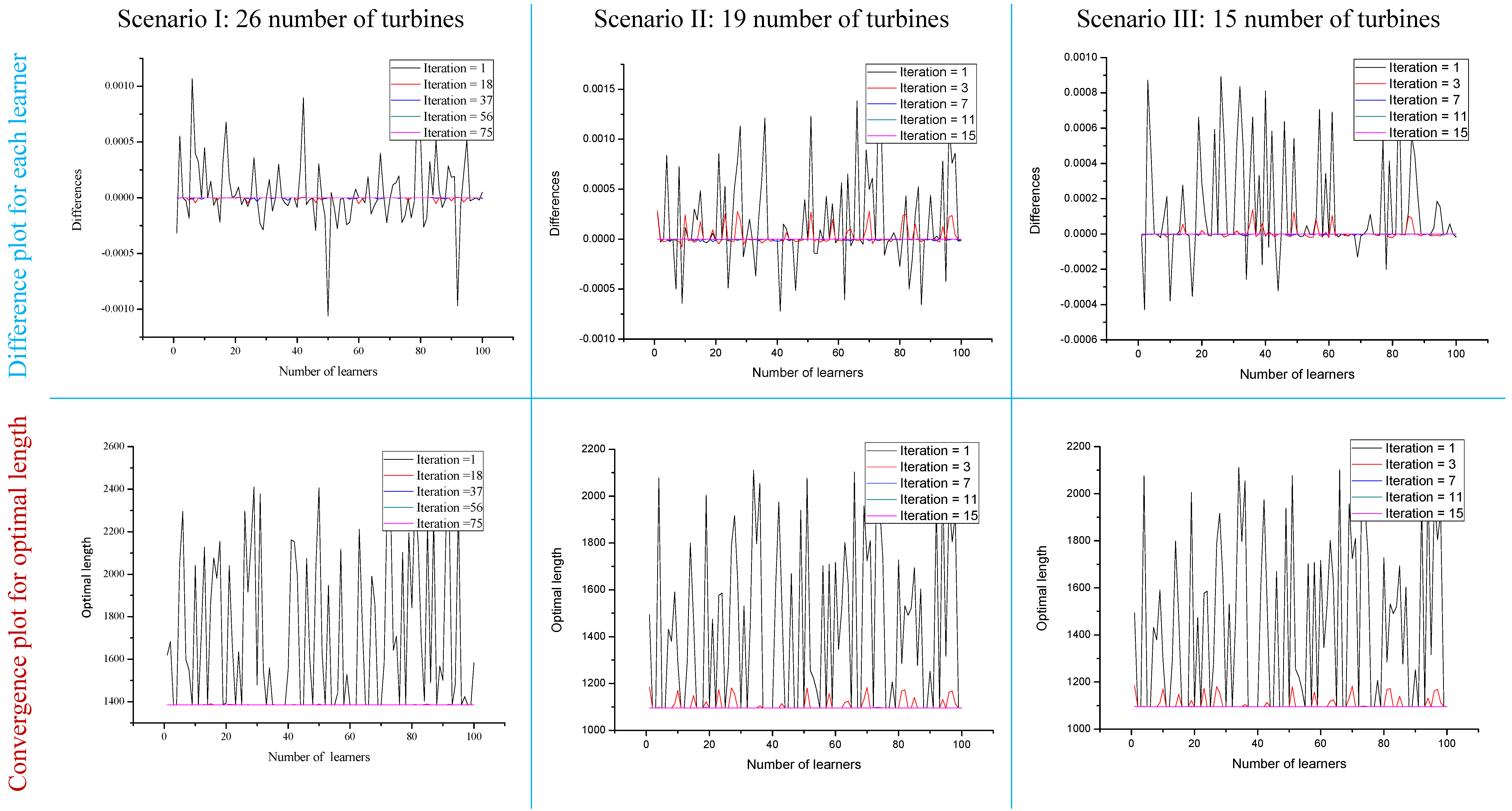
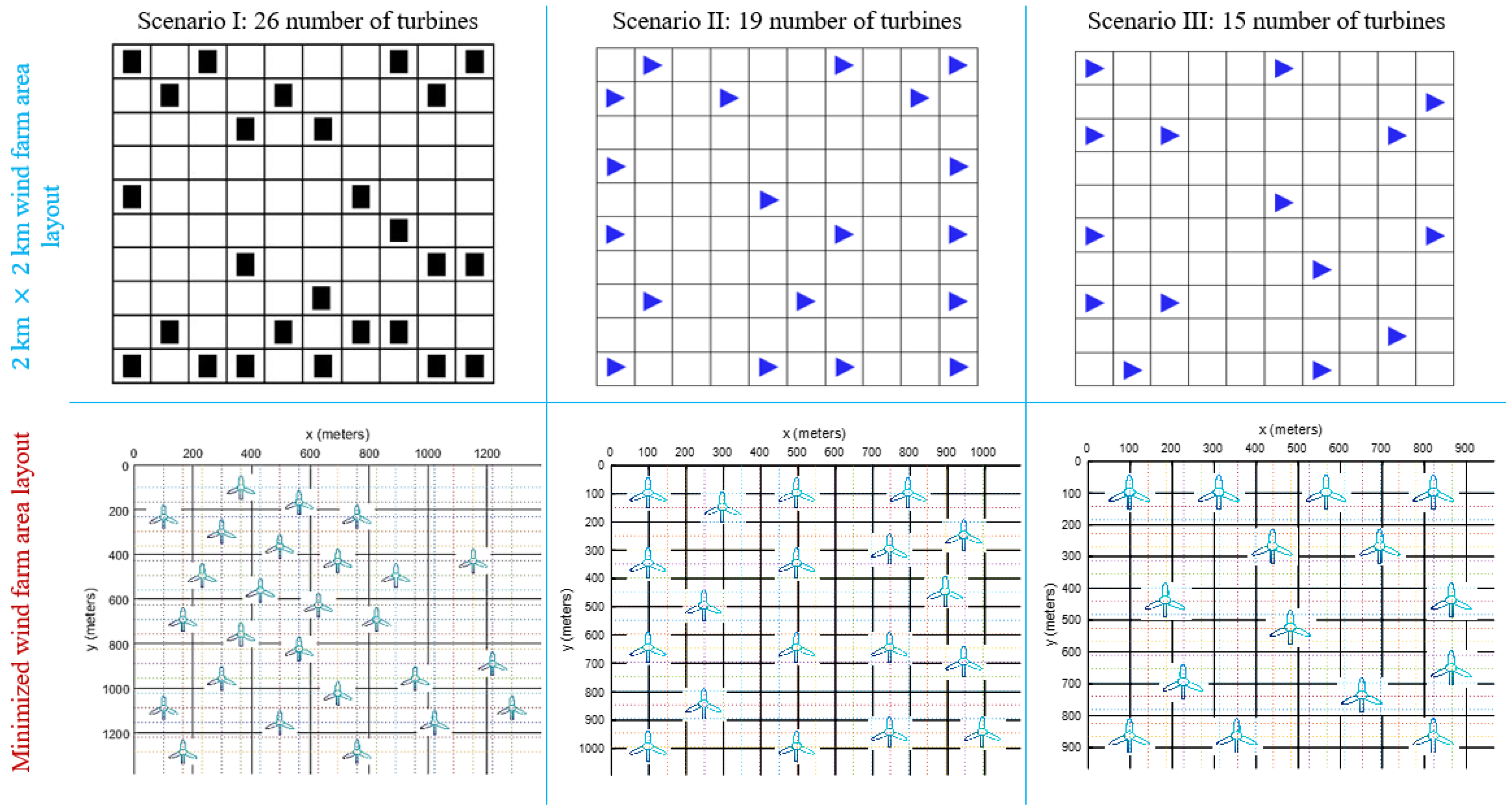
3.1. Case 1 vs. WFAO–ETLBO
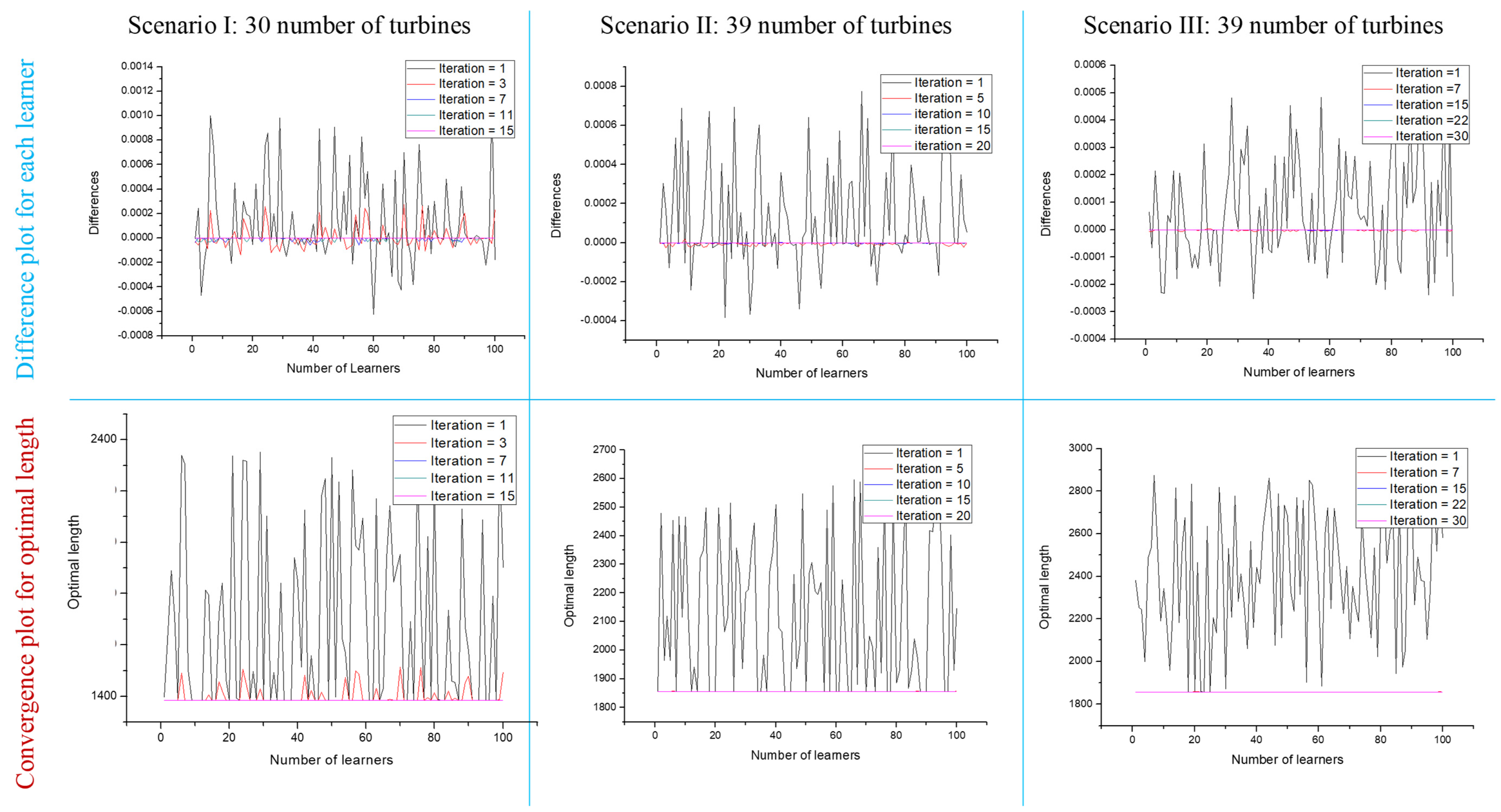
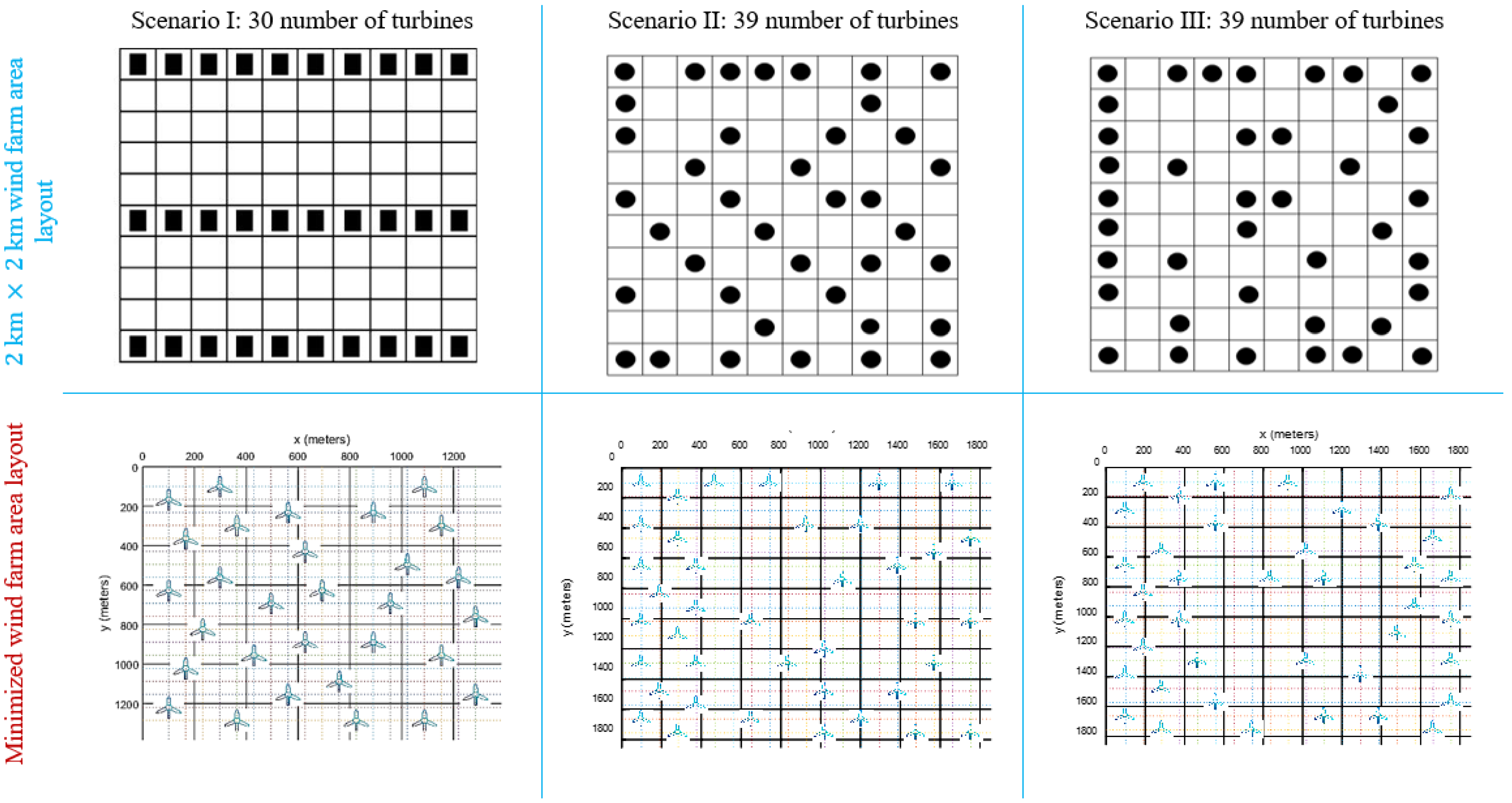
3.2. Case 2 vs. WFAO–ETLBO
3.3. Case 3 vs. WFAO–ETLBO
4. Conclusions
Author Contributions
Funding
Informed Consent Statement
Data Availability Statement
Acknowledgments
Conflicts of Interest
Nomenclature
| WFAO | Wind farm area optimization |
| ETLBO | Elitist Teaching–Learning-Based Optimization |
| undisturbed/freestream wind speed | |
| a | interference coefficient/induction/perturbation coefficient |
| rotor radius | |
| downstream rotor radius | |
| d | rotor diameter |
| x | wind downstream distance |
| wake spread angle | |
| entrainment constant | |
| K.E. | kinetic energy |
| N | number of turbines |
| P | actual power of wind turbine |
| ideal power of wind turbine | |
| density | |
| velocity of the turbine with multiple wake effect | |
| efficiency of wind farm | |
| power with multiple wake effects | |
| power without wake effects | |
| Lmean | Mean of a learner |
| Lteacher | Best learner identified as a teacher |
| Teaching factor | |
| Uniformly distributed random | |
| ith learner | |
| jth learner | |
| Fitness value of learner | |
| ε | convergence criteria |
| R.C. | relative change |
References
- Mosetti, G.; Poloni, C.; Diviacco, B. Optimization of wind turbine positioning in large wind farms by means of a genetic algorithm. J. Wind Eng. Ind. Aerod. 1994, 51, 105–116. [Google Scholar] [CrossRef]
- Grady, S.A.; Hussaini, M.Y.; Abdullah, M.M. Placement of wind turbines using genetic algorithms. Renew. Energy 2005, 30, 259–270. [Google Scholar] [CrossRef]
- Mittal, A.; Taylor, L.K. Optimization of Large Wind Farms Using a Genetic Algorithm. In Proceedings of the ASME 2012 International Mechanical Engineering Congress & Exposition, Houston, TX, USA, 9–15 November 2012. [Google Scholar] [CrossRef]
- Emami, A.; Noghreh, P. New approach on optimization in placement of wind turbines within wind farm by genetic algorithms. Renew. Energy 2010, 35, 1559–1564. [Google Scholar] [CrossRef]
- Jensen, N.O. A Note on Wind Generator Interaction; Technical Report Riso-M-2411; Risø National Laboratory: Roskilde, Denmark, 1983. [Google Scholar]
- Shakoor, R.; Hassan, M.Y.; Raheem, A.; Rasheed, N.; Mohd Nasir, M.N. Wind Farm Layout Optimization by Using Definite Point Selection and Genetic Algorithm. In Proceedings of the 2014 IEEE International Conference on Power and Energy (PECon), Kuching, Malaysia, 1–3 December 2014; pp. 191–195. [Google Scholar]
- Bastankhah, M.; Porte-Agel, F. A new analytical model for wind-turbine wakes. Renew. Energy 2017, 70, 116–123. [Google Scholar] [CrossRef]
- Kuo, J.Y.J.; Romero, D.A.; Amon, C.H. A mechanistic semi-empirical wake interaction model for wind farm layout optimization. Energy 2015, 93, 2157–2165. [Google Scholar] [CrossRef]
- El-Shorbagy, M.A.; Mousa, A.A.; Nasr, S.M. A chaos-based evolutionary algorithm for general nonlinear programming problems. Chaos Solit. Fractals 2016, 85, 8–21. [Google Scholar] [CrossRef]
- Chen, K.; Song, M.X.; Zhang, X.; Wang, S.F. Wind farm layout optimization using genetic algorithm with different hub height wind turbines. Renew. Energy 2016, 96, 676–686. [Google Scholar] [CrossRef]
- Turner, S.D.O.; Romero, D.A.; Zhang, P.Y.; Amon, C.H.; Chan, T.C.Y. A new mathematical programming approach to optimize wind farm layouts. Renew. Energy 2014, 63, 674–680. [Google Scholar] [CrossRef]
- Ituarte-Villarreal, M.; Espiritu, J.F. Optimization of wind turbine placement using a viral based optimization algorithm. Procedia Comput. Sci. 2011, 6, 469–474. [Google Scholar] [CrossRef] [Green Version]
- Ajit, P.C.; John, C.; Lars, J.; Mahdi, K. Offshore wind farm layout optimization using particle swarm optimization. J. Ocean. Eng. Mar. Energy 2018, 4, 73–88. [Google Scholar]
- Martina, F. Mixed Integer Linear Programming for new trends in wind farm cable routing. Electron. Notes Dis. Math. 2018, 64, 115–124. [Google Scholar]
- Gao, X.; Yang, H.; Lin, L.; Koo, P. Wind turbine layout optimization using multi-population genetic algorithm and a case study in Hong Kong offshore. J. Wind Eng. Ind. Aerod. 2015, 139, 89–99. [Google Scholar] [CrossRef]
- Eroglu, Y.; Seçkiner, S.U. Design of wind farm layout using ant colony algorithm. Renew. Energy 2012, 44, 53–62. [Google Scholar] [CrossRef]
- Feng, J.; Shen, W.Z. Solving the wind farm layout optimization problem using random search algorithm. Renew. Energy 2015, 78, 182–192. [Google Scholar] [CrossRef]
- Feng, J.; Shen, W.Z. Optimization of wind farm layout: A refinement method by random search. In Proceedings of the 2013 International Conference on Aerodynamics of Offshore Wind Energy Systems and Wakes, Copenhagen, Denmark, 17–19 June 2013. [Google Scholar]
- Wagner, M.; Day, J.; Neumann, F. A fast and effective local search algorithm for optimizing the placement of wind turbines. Renewable Energy 2013, 51, 64–70. [Google Scholar] [CrossRef] [Green Version]
- Yang, K.; Cho, K. Simulated Annealing Algorithm for Wind Farm Layout Optimization: A Benchmark Study. Energies 2019, 12, 4403. [Google Scholar] [CrossRef] [Green Version]
- Majid, K.; Shahrzad, A.; Mahmoud, O.; Forough, K.N.; Kwok, W.C. Optimizing layout of wind farm turbines using genetic algorithms in Tehran province, Iran. Int. J. Energy Environ. Eng. 2018, 9, 399–411. [Google Scholar] [CrossRef] [Green Version]
- Niayifar, A.; Porté-Agel, F. Analytical Modeling of Wind Farms: A New Approach for Power Prediction. Energies 2016, 9, 741. [Google Scholar] [CrossRef] [Green Version]
- Kusiak, A.; Zhe, S. Design of wind farm layout for maximum wind energy capture. Renew. Energy 2010, 35, 685–694. [Google Scholar] [CrossRef]
- Abdulrahman, M.; Wood, D. Wind Farm Layout Upgrade Optimization. Energies 2019, 12, 2465. [Google Scholar] [CrossRef] [Green Version]
- Roque, P.M.J.; Chowdhury, S.P.; Huan, Z. Performance Enhancement of Proposed Namaacha Wind Farm by Minimising Losses Due to the Wake Effect: A Mozambican Case Study. Energies 2021, 14, 4291. [Google Scholar] [CrossRef]
- Kirchner-Bossi, N.; Porté-Agel, F. Wind Farm Area Shape Optimization Using Newly Developed Multi-Objective Evolutionary Algorithms. Energies 2021, 14, 4185. [Google Scholar] [CrossRef]
- Hsieh, Y.Z.; Lin, S.S.; Chang, E.Y.; Tiong, K.K.; Tan, S.W.; Hor, C.Y.; Cheng, S.C.; Tsai, Y.S.; Chen, C.R. Wind Technologies for Wake Effect Performance in Windfarm Layout Based on Population-Based Optimization Algorithm. Energies 2021, 14, 4125. [Google Scholar] [CrossRef]
- Yeghikian, M.; Ahmadi, A.; Dashti, R.; Esmaeilion, F.; Mahmoudan, A.; Hoseinzadeh, S.; Garcia, D.A. Wind Farm Layout Optimization with Different Hub Heights in Manjil Wind Farm Using Particle Swarm Optimization. Appl. Sci. 2021, 11, 9746. [Google Scholar] [CrossRef]
- Al-Addous, M.; Jaradat, M.; Albatayneh, A.; Wellmann, J.; Al Hmidan, S. The Significance of Wind Turbines Layout Optimization on the Predicted Farm Energy Yield. Atmosphere 2020, 11, 117. [Google Scholar] [CrossRef] [Green Version]
- Bai, F.; Ju, X.; Wang, S.; Zhou, W.; Liu, F. Wind farm layout optimization using adaptive evolutionary algorithm with Monte Carlo Tree Search reinforcement learning. Energy Convers. Manag. 2022, 15, 115047. [Google Scholar] [CrossRef]
- Zilong, T.; Wei, D.X. Layout optimization of offshore wind farm considering spatially inhomogeneous wave loads. Appl. Energy 2022, 306, 117947. [Google Scholar] [CrossRef]
- Masoudi, S.M.; Baneshi, M. Layout optimization of a wind farm considering grids of various resolutions, wake effect, and realistic wind speed and wind direction data: A techno-economic assessment. Energy 2022, 244, 123188. [Google Scholar] [CrossRef]
- Porté-Agel, F.; Bastankhah, M.; Shamsoddin, S. Wind-Turbine and Wind-Farm Flows: A Review. Bound. Layer Meteorol. 2019, 174, 1–59. [Google Scholar] [CrossRef] [Green Version]
- King, R.N.; Dykes, K.; Graf, P.; Hamlington, P.E. Optimization of wind plant layouts using an adjoint approach. Wind. Energy Sci. 2017, 2, 115–131. [Google Scholar] [CrossRef] [Green Version]
- Antonini, E.G.A.; Romero, D.A.; Amon, C.H. Optimal design of wind farms in complex terrains using computational fluid dynamics and adjoint methods. Appl. Energy 2020, 261, 114426. [Google Scholar] [CrossRef]
- Dhoot, A.; Antonini, E.G.A.; Romero, D.A.; Amon, C.H. Optimizing wind farms layouts for maximum energy production using probabilistic inference: Benchmarking reveals superior computational efficiency and scalability. Energy 2021, 223, 120035. [Google Scholar] [CrossRef]
- Shakoor, R.; Hassan, M.Y.; Raheem, A.; Rasheed, N. Wind farm layout optimization using area dimensions and definite point selection techniques. Renew. Energy 2016, 88, 154–163. [Google Scholar] [CrossRef]
- Rao, R.V. Teaching-Learning Based Optimization and Its Engineering Applications; Springer: London, UK, 2015. [Google Scholar]
- Ammar, A.; Ahmad, S.I. Teaching-learning based optimization algorithm for core reload pattern optimization of a research reactor. Ann. Nucl. Energy 2019, 133, 169–177. [Google Scholar] [CrossRef]
- Rao, R.V.; Patel, V. An elitist teaching-learning-based optimization algorithm for solving complex constrained optimization problems. Int. J. Ind. Eng. Comput. 2012, 3, 535–560. [Google Scholar] [CrossRef]
- Rao, R.V.; Patel, V. Comparative performance of an elitist teaching-learning based optimization algorithm for solving unconstrained optimization problems. Int. J. Ind. Eng. Comput. 2013, 4, 29–50. [Google Scholar] [CrossRef]
- Rao, R.V.; Savsani, V.J.; Vakharia, D.P. Teaching-learning-based optimization: A novel method for constrained mechanical design optimization problems. Comput.-Aided Des. 2011, 43, 303–315. [Google Scholar] [CrossRef]


| Scenario-I | Scenario-II | Scenario-III | ||||
|---|---|---|---|---|---|---|
| Mosetti et al. | WFAO–ETLBO | Mosetti et al. | WFAO–ETLBO | Mosetti et al. | WFAO–ETLBO | |
| Number of turbines | 26 | 26 | 19 | 19 | 15 | 15 |
| Number of individuals | 200 | 100 | 200 | 100 | 200 | 100 |
| Fitness value | 0.001619 | 0.0015868 | 0.0017371 | 0.0019232 | 0.00099405 | 0.0010977 |
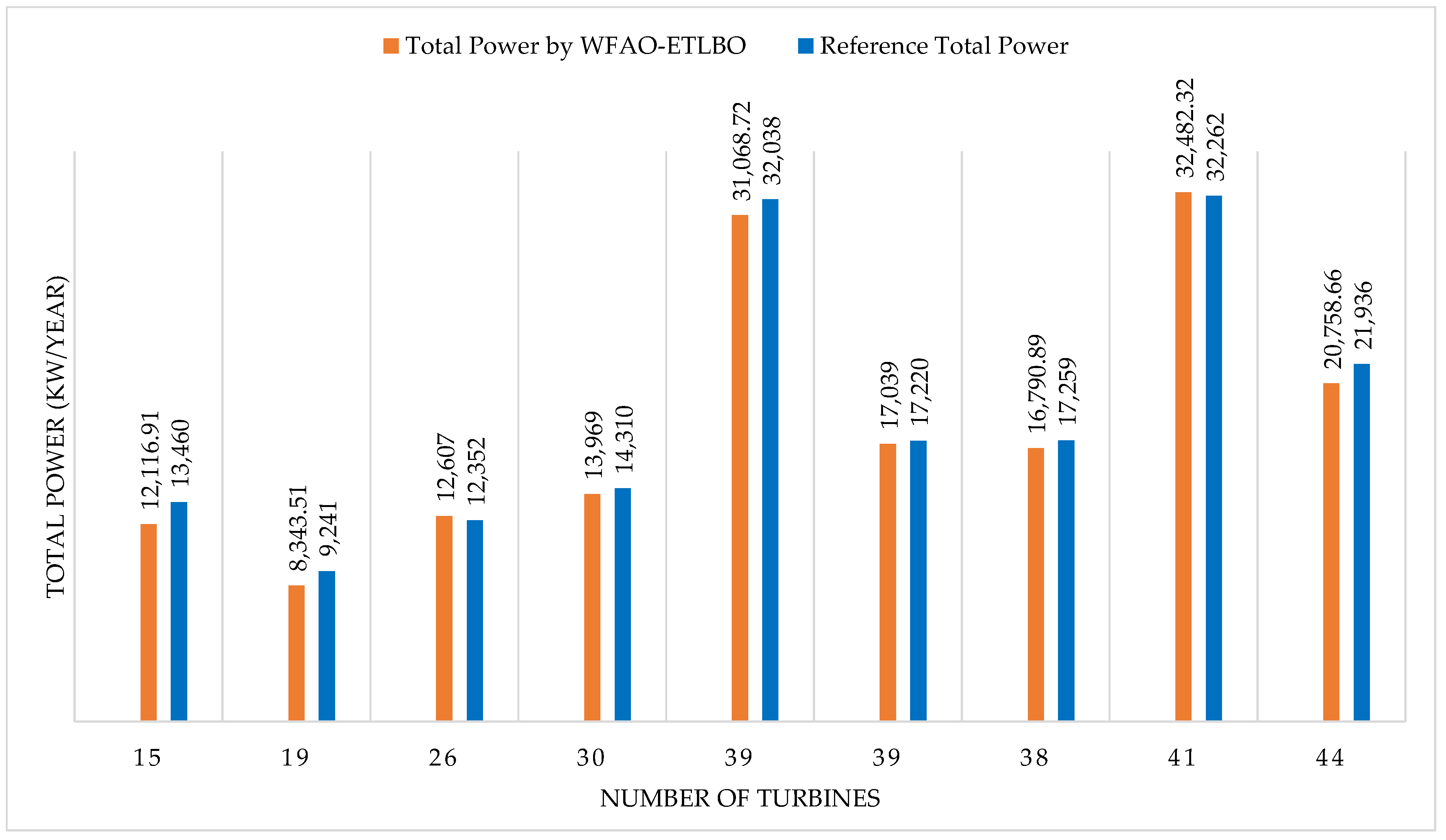
| Total Power (KW/year) (R.C. (%)) | 12,352 | 12,607.9 (2.07) | 9244 | 8343.51 (9.74) | 13,460 | 12,116.91 (9.97) |
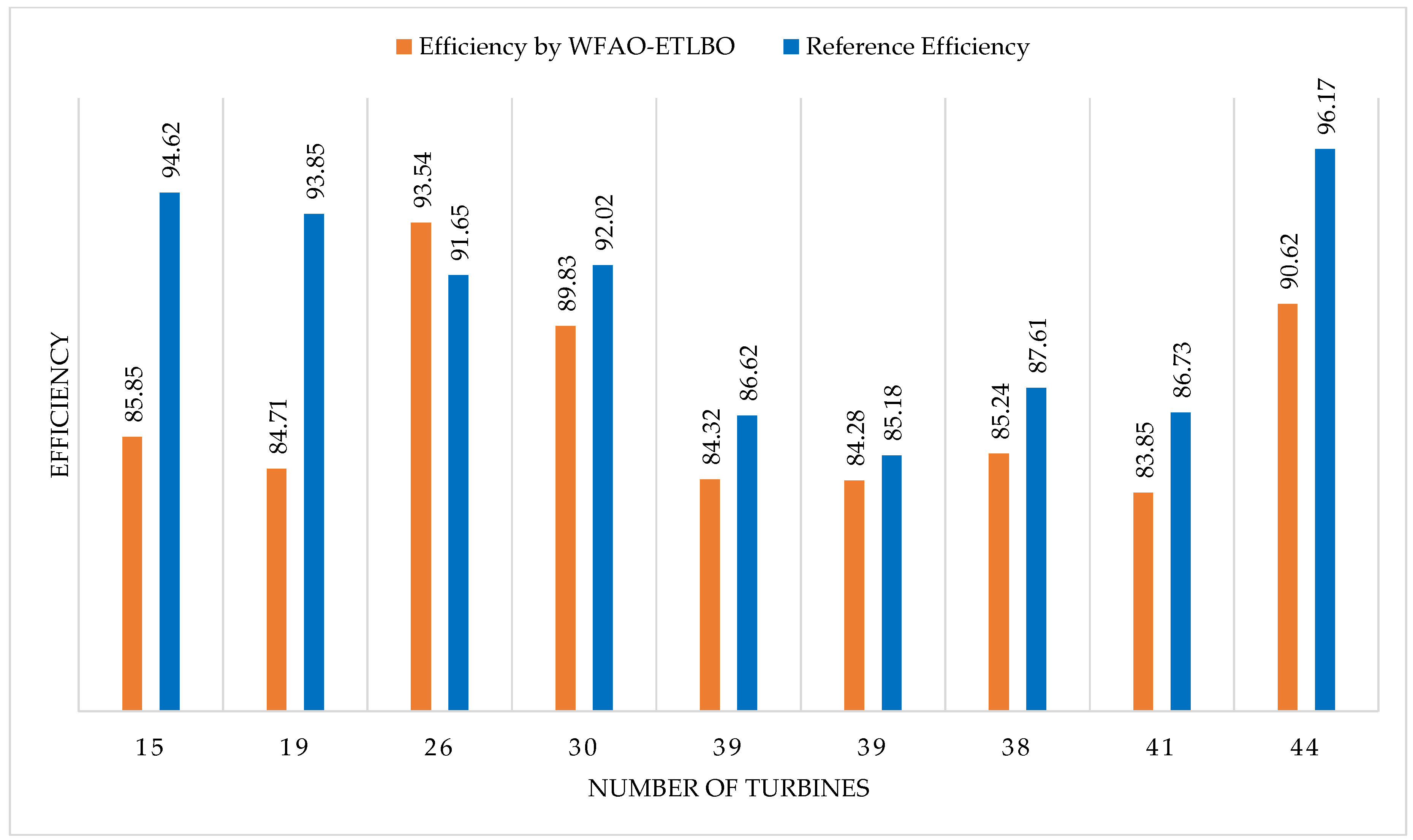
| Efficiency (%) (R.C. (%)) | 91.65 | 93.54 (2.07) | 93.851 | 84.71 (9.74) | 94.62 | 85.85 (9.26) |
| Converged number of iterations | 400 | 75 | 350 | 15 | 400 | 15 |
| Area Used (m) | 2000 × 2000 | 1385 × 1385 | 2000 × 2000 | 1095 × 1095 | 2000 × 2000 | 966 × 966 |
| % Reduction in Area | ~ | 30.75 | ~ | 45.25 | ~ | 51.75 |
| Simulation Time (s) | Not reported | 480.2 | Not reported | 708.7 | Not reported | 534.5 |
| Scenario-I | Scenario-II | Scenario-III | ||||
|---|---|---|---|---|---|---|
| Grady et al. | WFAO–ETLBO | Grady et al. | WFAO–ETLBO | Grady et al. | WFAO–ETLBO | |
| Number of turbines | 30 | 30 | 39 | 39 | 39 | 39 |
| Number of individuals | 600 | 100 | 600 | 100 | 600 | 100 |
| Fitness value | 0.0015436 | 0.0015812 | 0.0015666 | 0.0015800 | 0.0008403 | 0.0008665 |
| Total Power (KW/year) (R.C. (%)) | 14,310 | 13,969.59 (2.37) | 17,220 | 17,039.24 (1.05) | 32,038 | 31,068.72 (3.02) |
| Efficiency (%) (R.C. (%)) | 92.015 | 89.83 (2.37) | 85.174 | 84.28 (1.05) | 86.619 | 84.32 (2.65) |
| Converged number of iterations | 1203 | 15 | 3000 | 20 | 1000 | 30 |
| Area Used (m) | 2000 × 2000 | 1385 × 1385 | 2000 × 2000 | 1856 × 1856 | 2000 × 2000 | 1856 × 1856 |
| % Reduction in Area | ~ | 30.75 | ~ | 7.2 | ~ | 7.2 |
| Simulation Time (s) | Not reported | 134.86 | Not reported | 4978.29 | Not reported | 4101.44 |
| Scenario-I | Scenario-II | Scenario-III | ||||
|---|---|---|---|---|---|---|
| Mittal et al. | WFAO–ETLBO | Mittal et al. | WFAO–ETLBO | Mittal et al. | WFAO–ETLBO | |
| Number of turbines | 44 | 44 | 38 | 38 | 41 | 41 |
| Number of individuals | Not reported | 100 | Not reported | 100 | Not reported | 100 |
| Fitness value | 0.0013602 | 0.0015101 | 0.0015273 | 0.0015699 | 0.00084379 | 0.0008641 |
| Total Power (KW/year) (R.C. (%)) | 21.936 | 20,758.66 (5.36) | 17,259 | 16,790.89 (2.71) | 33,262 | 32,482.32 (2.34) |
| Efficiency (%) (R.C. (%)) | 96.17 | 90.62 (5.77) | 87.612 | 85.24 (2.71) | 86.729 | 83.85 (3.32) |
| Converged number of iterations | Not reported | 23 | Not reported | 15 | Not reported | 20 |
| Area Used (m) | 2000 × 2000 | 1856 × 1856 | 2000 × 2000 | 1856 × 1856 | 2000 × 2000 | 1856 × 1856 |
| % Reduction in Area | ~ | 7.2 | ~ | 7.2 | ~ | 7.2 |
| Simulation Time (s) | Not reported | 94.51 | Not reported | 1950.44 | Not reported | 3002.15 |
Publisher’s Note: MDPI stays neutral with regard to jurisdictional claims in published maps and institutional affiliations. |
© 2022 by the authors. Licensee MDPI, Basel, Switzerland. This article is an open access article distributed under the terms and conditions of the Creative Commons Attribution (CC BY) license (https://creativecommons.org/licenses/by/4.0/).
Share and Cite
Hussain, M.N.; Shaukat, N.; Ahmad, A.; Abid, M.; Hashmi, A.; Rajabi, Z.; Tariq, M.A.U.R. Micro-Siting of Wind Turbines in an Optimal Wind Farm Area Using Teaching–Learning-Based Optimization Technique. Sustainability 2022, 14, 8846. https://0-doi-org.brum.beds.ac.uk/10.3390/su14148846
Hussain MN, Shaukat N, Ahmad A, Abid M, Hashmi A, Rajabi Z, Tariq MAUR. Micro-Siting of Wind Turbines in an Optimal Wind Farm Area Using Teaching–Learning-Based Optimization Technique. Sustainability. 2022; 14(14):8846. https://0-doi-org.brum.beds.ac.uk/10.3390/su14148846
Chicago/Turabian StyleHussain, Muhammad Nabeel, Nadeem Shaukat, Ammar Ahmad, Muhammad Abid, Abrar Hashmi, Zohreh Rajabi, and Muhammad Atiq Ur Rehman Tariq. 2022. "Micro-Siting of Wind Turbines in an Optimal Wind Farm Area Using Teaching–Learning-Based Optimization Technique" Sustainability 14, no. 14: 8846. https://0-doi-org.brum.beds.ac.uk/10.3390/su14148846