1. Introduction
Photovoltaic (PV) power, wind turbine energy and other renewable energy sources (RES) will be used to a significantly high extent due to the Paris agreement in 2015 to globally reduce greenhouse gas emissions [
1]. A crucial point in the renewable energy power system among distributed energy resources (DERs) is the photovoltaic system (PVS) because of the flexibility of PVS installation on the small or medium scale in residences, public buildings, factories, etc. Photovoltaics starts to displace the conventional generation. Regarding the renewable energy portfolio standard for many states and countries around the world, PVS is tending toward becoming one of the fundamental forms of renewable energy [
2,
3].
However, PVS is dependent on the linear nature of sunlight to aim for constant output. In the real situation, this condition cannot be obtained because of the high variability of sunlight. Therefore, protection such as stability, reliability and operation of the PVS from the grid is needed when unsuitable conditions occur [
4,
5]. Several supports are important to verify good features of (PV) characteristics while injecting power facing to the grid. The grid sensitivity increases when an abnormal situation occurs caused by the penetration of the PVS. Grid code (GC) requirements have also been modified in many countries due to increasing penetration of PV into the grid [
6,
7,
8]. During a fault condition, the inevitable changes occur in the network’s basic parameters, including some grid parameters, namely voltage, current, transmission power and frequency. Moreover, the steadiness of the grid parameters is accomplished using reactive current insinuate to reinforce and stabilize the grid voltages during fault conditions. In addition, for voltage support, RES must inject reactive current equivalent around 2% of the nominal current whenever the inverter voltage drops below the voltage standard. Voltage supports have to be enforced within 20 ms after an abnormality is distinguished in the network system, which induces a full reactive current support when voltage sagging reaches half or higher than the rated voltage [
9]. Recently, TSOs launched a grid code in which the REN source is forcibly connected to the utility part under all operating conditions [
9]. Applying these grid codes improves the stability of the power system. The most important code is to ensure that PVS can reconnect within the minimum time range after a voltage drop and fixes the grid rated voltage. Alternatively, this situation can be classified as a low voltage ride pass (LVRT) function. Additionally, some literatures have proposed methods regarding the fault ride through (FRT) control strategies capability; the requirements of an off-grid FRT system’s grid code such as voltage and frequency with high penetration of RES are used for reference study. The LVRT capability can be obtained by injecting reactive power during a temporary unbalanced grid system [
10].
High penetration of renewable energy sources, such as German energy companies known as Energy On (E.ON) and Comitato Electrotecco Italiano (CEI), modified national grid requirements for PVS, which were introduced with low voltage ride through (LVRT) capacity. The LVRT capabilities are illustrated by countries such as Denmark, Germany, Italy, Spain and the USA, which have a significant amount of power generation [
11]. In July 2010, the German grid code stipulated that PV power plants should be able to contribute limitedly to dynamic network support, and since January 2011, PVS has recommended dynamic network support in the event of an accident. In the PCC study of a Category 2 power plant, the voltage limit curve was defined by E.ON. Italy recently adopted a new grid code version for distributed power generation systems including PV. Japan announced FRT requirements and countermeasures for the PV distribution system by the Energy Industry Development Organization (NEDO) in 2011. The United States has applied the IEEE 1547 standard and regulation of PV integration in accordance with technical requirements for wind and solar interconnection at Puerto Rico’s power plant [
12].
During abnormalities in the power system, several references of FRT strategies such as a crowbar, resistance superconducting fault current limiters (RSFCLs) and another type of fault current limiter were proposed to minimize current value and improve power quality. For example, it minimizes oscillations for wind turbine applications [
13,
14]. According to this evaluation study [
15,
16] on asymmetric and unbalanced failures, active and reactive power current control is performed. In addition, despite this criterion [
15], positive and negative sequence from flexible active power balance control are proposed. Moreover, according to these references [
17,
18] several FRT strategies such as STFCL and BFCL were investigated compared to a conventional crowbar during an asymmetrical fault condition. Furthermore, the value of the grid parameter could be reached according to grid code through the new design of the proposed controller. The depth comparison regarding topology for each controller was discussed, and the main reason for grid the working principle of topology. STFCL circuitry consists of a fault parameter improvement value illustrated through a current limiting inductor and resistance for each phase to suppress voltage transients during fault initiation as well as a series branch of resistance and inductance as a path for energy absorption during the fault period. Meanwhile, BFCL circuitry is the combination of two paths; the first path is called the bridge path, which works during normal situations without fault conditions. The bridge path consists of up to four bridge diodes, which are responsible to the positive and negative cycle of alternating current variables. Another path is called the shunt path, which consists of resistance and inductance to control the power flow during fault conditions. Furthermore, until now there has been no in-depth comparison regarding limitations of both FRT strategies for grid-connected PVS during asymmetrical fault.
However, most of the studies described FRT strategies combined with proportional integration (PI) and proportional resolution (PR) as the inverter control to meet the LVRT functionality. Simple PI controllers have many applications at the industrial level, but there are several restrictions due to their sensitivity to parametric variables and nonlinear behavior in dynamic environments (e.g., disturbance conditions and parametric uncertainty). According to [
19], fuzzy logic controller (FLC) based on steepest descent (SD) was applied for induction motor as an objective study. The advantage of the SD optimization algorithm is that it is adequate for multi-input–multioutput (MIMO) systems and decreases the error of linear and nonlinear functions. Moreover, the performance assessment using FLC-based SD described a great improvement value. Furthermore, until now there has been no in-depth comparison regarding the application of FLC-based SD as the inverter control combined with FRT strategies for grid-connected PVS during asymmetrical fault.
To overcome these issues, we present the proposed FRT strategy, i.e., bridge-type fault current limiter BFCL as the FRT scheme with the FLC-based steepest descent (SD) method as the inverter control to maximize the PVS parameters under contingency affections compared to STFCL along with conventional inverter control, i.e., PI controller. Moreover, three combinations of FRT strategies and inverter control such as PI + STFCL, PI + BFCL and SD + BFCL are introduced in this paper. A deep comparison is carried out with several proposed combination strategies between inverter and FRT strategies during asymmetrical faults. In addition, the robustness of other electrical parameters such as DC link voltage, grid voltage and grid active power response is illustrated. The contributions of the paper are listed below:
Analysis of the grid-connected PVS with specifications 100 kW MATLAB/Simulink model is carried out, i.e., grid side parameters are evaluated in accordance with the acceptance limits focused on PCC during asymmetrical fault.
A novel switch-type fault current limiter (STFCL) and bridge-type fault current limiter (BFCL) strategy is implemented to refine the LVRT operation.
A detailed and keen comparison of BFCL with STFCL topology is performed.
FCL-based steepest descent algorithm method (SD) is delineated and in contrast to formerly practiced PI controllers.
Scenario of asymmetrical faults are used for 200 ms to authenticate LVRT operation of proposed SD + BFCL along with STFCL in comparison to the conventional PI strategy.
There are performance evaluation analysis characteristics such as integral absolute error (IAE), integral square error (ISE) and integral of time-weighted absolute error (ITAE) are enforced to evaluate steadiness of the suggested controller and strategy.
The other sections are described as follows:
Section 2 discusses the Photovoltaic cell, DC boost converter, inverter and proposed system mathematical modeling.
Section 3 discusses the proposed model and inverter controller design and FRT as a plan of action. Moreover, several FRT results schemes and a description of the FRT discussion are covered in
Section 4, and the conclusion of study is found in
Section 5.
2. Materials and Methods
In this paper, the model proposed for applying FCL to PV system in power system is described below:
2.1. Mathematical Modeling of Photovoltaic Cell
The mathematical modeling of the PV cell used in the simulation becomes the equivalent circuit of the
Figure 1. The equivalent circuit of a PV cell consists of a current source, a diode, a parallel resistor Rp and a series resistor Rs. The output current of a PV cell can be calculated as follows using Kirchhoff’s current law:
where,
= PV cell voltage (V)
= thermal voltage (V)
= PV cell output current (A)
= PV light current (A)
= diode reverse saturation current (A)
series resistance (Ω)
= shunt resistance (Ω)
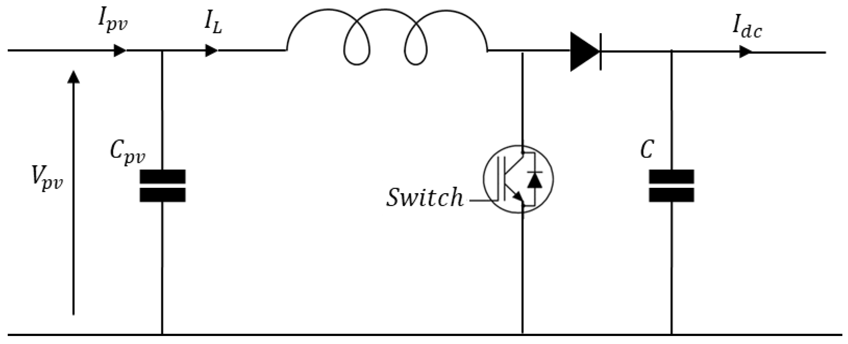
2.2. Mathematical Modeling of DC–DC Boost Converter
As illustrated in
Figure 2, most PV power plants connected to the power grid use DC–DC boost converters for boosting the voltage parameters. The mathematical modeling of the DC–DC boost converter is presented through Equation (3). The boost converter uses the voltage as a duty ratio that is an on/off period through a switch operation. MPPT (maximum power point tracking) control is used to relieve sensitive variability characteristics of PV while boosting voltage to supply maximum power. The parameter
connected in parallel to the PV stage needs to be set through the following equation to minimize the harmonics situation:
D = duty ratio
= PV array output voltage = 273 V
= switching frequency = 5 kHz
= boost inductor = 5 Mh
input voltage (PV array output voltage) = 273 V
= output voltage of DC–DC boost converter = 500 V
2.3. Modeling of Inverter
An inverter is a power electronic device that converts DC voltage into AC voltage. There are two types of inverters, voltage-type inverters, and current-type inverters. In this paper, since most loads require a constant voltage, a voltage-type, 3-phase grid-connected inverter is used. The 3-phase grid-connected inverter was simulated using 6 IGBT switches. The inverter controls the voltage and current while independently controlling
by converting the values obtained by measuring the PCC stage of the system into the d-q frames of Equations (6) and (7). The PWM signal used at this time generates PWM using the voltage obtained from the current controller, thereby generating an inverter gate pulse signal.
2.4. Mathematical Modeling of STFCL Circuit
According to [
20], PI-STFCL is compared to the Modified STFCL; the result showed that both models have a good fault recovery performance and signifies an enhanced LVRT for the balance and secure the operation of wind farm. However, in this case, Modified STFCL is more superior for reactive power support during disturbances. In addition, the mathematical modeling of STCL could be explained through [
21]. As illustrated in this study, the STFCL modeling in the DFIG system is made according two operation strategies, i.e., normal and voltage transient operation. Moreover, mathematical modeling of STFCL with the PV system could be described through Equations (8) and (9).
The voltage equation for normal mode is expressed as:
where
:
2.5. Mathematical Modeling of BFCL Circuit
According to [
22], during the fault condition on FSWT, BFCL improves transient behavior of the system instantly. In this case, the system is a fixed-speed wind turbine connected to the grid, and the author was using a proportional–integral (PI) controller to regulate the DC reactor current. However, mathematical modeling of BFCL with the PV system could be described through Equations (10) and (11).
The source impedance is described as:
The line and load model impedance is expressed as:
2.6. Description of PV Array
In this section, we discuss the PV array system parameter, which is described according to
Table 1. As described in this table, the power rating of the PV array system is 100 kW. Moreover, the detail specifications of an operation with PV array, grid and local load are expressed in further sections.
2.7. Description of Block Diagram Test System and Fault Location
2.7.1. Proposed Test System
As illustrated in
Figure 3, the proposed FRT circuitry and inverter control, i.e., BFCL and the FLC-based SD algorithm, is added to power system simulation using SimPower examples of the MATLAB/Simulink software. The maximum voltage of the PV array is 273 V, the frequency of the DC–DC boost converter (blue shaded region) is 5 kHz, and the output voltage is 500 V. The control structure of the inverter (inside red-shaded region) three-level VSC is applied to optimize DC link voltage. Two inverter control loops (white-shaded region) are depicted: the internal control loop has a function to maintain reactive
and real components
ordinance of the grid and two capacitors to +/− 250 V, which is used to adjust the DC link voltage at the external loop function. As reference, the value of the DC link controller voltage is set to 500 V. The output
d-q frame is recreated in several modulating signals with the PWM generator application at the current controller part (inside white-shaded region).
MPPT control (inside blue-shaded region) is performed by the DC–DC converter to adjust the duty ratio of the DC–DC converter. The switching frequency value of inverter (red-shaded region) is 2 kHz, which will convert to 260 V AC. The system proceed after the AC voltage is converted by the inverter, passes through the LCL filter and then passes through the FRT circuit to reach the load stage. Two different inverter controllers, PI and FLC-based SD algorithm, which are shown in
Figure 3a (inside white-shaded region) and
Figure 3b (inside green-shaded region) are used to optimize the network problem, namely current and power limiting, voltage sag, etc. The simulation of asymmetrical grid faults takes place at the PCC, which is discussed in more detail in
Section 2.7.2.
2.7.2. Description of Fault Location Test System, Grid and Local Load
In order to explain in more detail about the fault location, the subsystem of the load stage with connection from the other grid is presented. Moreover, the low-voltage subsystem part with the transformer device are illustrated in
Figure 4. The network system impedance could be described according to the amount of impedance between the point of common coupling (PCC) and the transformer point of the other grid. In this case study, the value of impedance is 8.511 Ω. Moreover, the internal impedance of the inverter (red-shaded region) model could be neglected due to a small value of impedance around 0.0002 Ω. The parameters of grid and local load are illustrated in
Figure 4. The grid parameter consists of four blocks: a step-down transformator, point of interconnection, three-phase breakers and the source capacity, which has a parameter of 110 kV 2500 MVA.
3. Proposed Inverter Control and FRT Methods
In the previous section, we discussed several FRT strategies applied to the grid. This section elaborates on the proposed FRT strategies and inverter controller method, i.e., bridge-type fault current limiter (BFCL) along with steepest descent (SD).
3.1. Switch-Type Fault Current Limiters (STFCL)
As mentioned in the introduction, the LVRT characteristics are crucial for several requirements for grid code of TSOs. Currently, the current limiter’s characteristic is a viable option to improve the fault current limiter’s characteristic. Thus, it is inevitable to compromise on the protection of the power system during fault conditions. Therefore, until now various control and electronic-based strategies have been presented for the reliable and stable operation of the power system. Below, the working principle of the proposed STFCL is discussed. The conventionally used crowbar circuit includes pure resistance in the path of fault current. The STFCL circuitry was designed for a doubly fed induction-generator (DFIG) [
17]. STFCL circuitry is composed of two operations, which will be used to optimize voltage surges when switching periods, and a path for fault energy absorption, as depicted in
Figure 3. In the first operation regarding the switching period, fault current limiting inductors (
) and resistance (
), in series for each phase, a full-bridge rectifier, linear transformers, power electronic switches and a snubber capacitor (
), are enforced. In the second operation regarding the absorbing period, a series branch of
and
in parallel with the snubber capacitor is applied. Moreover, the switch (SW) remains on at normal conditions and bypasses the fault current limiting inductors and resistance path. However, during any abnormal conditions, the SW turns off.
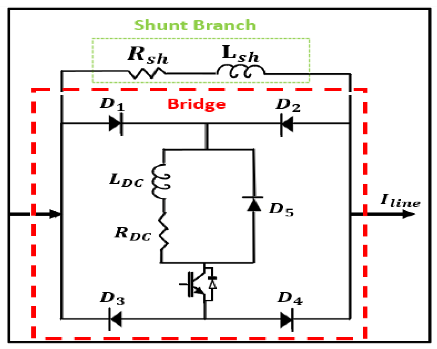
3.2. BFCL (Bridge-Type Fault Current Limiter)
BFCL consists of two elements, a bridge part and a shunt branch part, and since it does not require a superconducting feature, the application cost is low compared to other current limiting devices. The bridge consists of 4 diodes, and . The IGBT switch and internal and exist inside the bridge. The role of is for the safe operation of . and placed in parallel with the bridge circuit exist. The resistance value of these two becomes ().
As shown in
Figure 5 during normal operation of BFCL, the IGBT element is turned on, and current flows in the path of
in the positive half cycle of the signal and in the path of
in the negative half cycle. Through this process, a current in the same direction flows through the
during the period of the electric frequency, and the previous current becomes a direct current. At this time, the
is charged up to the peak of the current, and the voltage drop of the diodes is significantly smaller than the line voltage drops, so it can be ignored, and it can be confirmed that it operates as a short circuit. BFCL becomes a circuit that does not affect the system in a steady state. Since the resistance of the shunt branch is set to a very large value, a normal current flows to the bridge except for a small amount of leakage current. As depicted in
Figure 6 in the case of BFCL fault, if the set excess current flows to
, IGBT turns off. When the IGBT is off, the bridge circuit becomes an open circuit. Then the shunt branch is reset to the path, and the current is limited because it is a path with high impedance. Thus, when the IGBT is turned on again after the fault, the free-wheeling diode of
creates a path to consume the residual reactor current of the
, thereby preventing high switching current during IGBT operation.
3.3. The Description of Inverter Controller Modeling
Several FRT strategies were designed to protect the PV power source from multiple fault conditions in the system. The basic control method is to stably manage the DC link from the PV. However, problems such as normal power, voltage, current, power factor and phase occur in a fault condition, so a controller that optimizes system parameters is required. In this paper, we propose a method using PI and SD controllers as control methods and STFCL and BFCL as FRT strategies.
Inverter Control Modeling
The proposed control method for stably adjusting the power of the voltage-type inverter will be described as follows. The keen comparison between the conventional algorithm method and the proposed algorithm method is explained through some equation and topology modeling.
The block diagram in
Figure 7 is a method of adjusting and comparing the DC link voltage using the PI controller. When the current is converted to a d-q frame, the d-axis and q-axis values become DC, which makes it easy to control and filter. The output controlled by
and
is set to 0 to maintain the power factor. Through the internal controller,
and
make PWM control, the sign of asterisk (*) describe as a reference value.
- 2.
Steepest Descent Method.
The main characteristic of the SD controller is small step sizes; due to this reason, the result of the controller is slowly presented to estimate the grid-connected inverter. The discrete time is enforced to illustrate the convergence parameter status of inverter-side currents and voltage. For regularization term control, several mathematical equations according to [
19,
23] are applied to define the stability standard and minimum point.
As illustrated in
Figure 8, the SD controller has four types of the modeling process. Fuzzification modeling is utilized with the intent to maps two types of data, i.e., real or crisp type according to the fuzzy set system, which considers several parts, e.g., fuzzy linguistic variables as the main part, linguistic terms for the secondary part and membership functions remarkable as the tertiary part. A “rule base” consists of IF–THEN rules with a conclusion and condition. In addition, “rule base” defines the action by adjusting the output value of variable controller. Inference mechanism modeling is applied to find the optimum parameter by computation based on the gradient steepest descent method. The output parameter such as grid voltages can be effectively estimated from the inference mechanism into crisp/real-time output according to [
24]; the other parameters are also estimated using defuzzification as described in
Figure 8.
- 3.
The Equation for Controller Output
In these studies, we integrated the SD algorithm with fuzzy logic control (FLC) to optimize and utilize MIMO (multi-input–multioutput) topology as well as significantly reduce the error of linear and nonlinear functions. This explanation is described through Equation (12), which is also integrated with the cost function formula according to [
17], as follows:
where the MF “central of gravity” of the defuzzification technique is used to find the output value, as below:
Reflected to the MF of value output variable, the input and output of the combined proposed method based on the SD algorithm are updated through Equation (13). The MF is used in the design of the Gaussian membership function (GMF) as an alternative to trapezoidal, triangular and generalized bell. The center and variance are two iterative parameter constraints that GMF needs to utilize to achieve two main targets, i.e., a fewer number of parameters, and works well during continuous function.
- 4.
Jacobian Calculation
Through Equation (12), each parameter of the Jacobian matrix such as center, MF and variance could be calculated using cost function of partial derivative concept, which is reflected in the (w.r.t) parameter. Cost function (w.r.t) output
is as follows:
The following equations are obtained after submitting GMF values.
The Jacobian of Gaussian output MF is described through Equation (17). In addition, the Jacobian parameters such as center ( and variance can be illustrated by using the partial derivative of cost function through Equation (12), respectively. Furthermore, through derivative cost, Equations (12)–(17), with regard to and , depict the Jacobian of GMF output along with center and variance, respectively.
- 5.
Final Equations for FLC–SD Algorithm
The proposed controller based on the FLC and SD algorithm can be called error back-propagation due to the characteristic, which utilizes first derivative order. The updated equation for two parameters of GMF constraints, i.e., center and variance, as well as output MP, are defined, respectively, as:
Based on this equation we can conclude that SD algorithm training is asymptotic convergence. Where is the gradient and is step size or learning rate constant. Other parameters are almost similar such as variance and center (. Output membership function update equations are practically similar according to the EBP adaptation rules. Moreover, the steepest descent algorithm training process is asymptotic convergence.
4. Results and Discussion
The FRT and inverter proposed control (i.e., BFCL and SD) are conducted through analysis and comparison with existing PI and STFCL FRT strategies. The scenario for case studies is described around 0.6 s. The main reason the short time was applied is due to the protection characteristic of the FRT in the system. Moreover, in [
9], grid parameter must be established within 20 ms after fault situation. The other crucial goal is to ensure that the PVS could reconnect within the optimum time, e.g., minimum duration range after grid voltage drop. In addition, to achieve all goals, the fault in the grid is simulated for 200 ms, which is applied in 0.2 s through this simulation. The fundamental behavior and comparison of the proposed and the existing approaches are discussed graphically and analyzed through the following performance measurements.
4.1. Performance Evaluation Indices
The performance evaluation indices are used in the following simulation for evaluating control performance. There are three indicators, IAE, ISE and ITAE. With these three indicators, the performance of the PI and SD controllers is evaluated, and the combined FRT strategy is compared precisely and accurately. The smaller value in evaluation indicates better performance.
ISE (integral square error): ISE is integrated by squaring the error over time. The smaller the value of ISE, the faster the control system will clear the error. The fact that it is the square of the error makes it possible to remove the error quickly. On the other hand, very small errors have the characteristic of remaining unresolved.
Mathematically,
IAE (integral absolute error): IAE is integrated after replacing the error with an absolute value over time. Since IAE calculates only the absolute value of the error, the weight of the error is not applied. Since there is no weight applied, there is a tendency of a rather slow error removal, but there is a characteristic that even small vibrations are removed.
Mathematically,
ITAE (integral time-weighted absolute error): The ITAE is an integral form of the IAE by additionally multiplying it by time. This includes an increasing weight for errors over time.
Mathematically,
4.2. Single Phase to Ground (S-G) Fault
The single phase to ground is approached to determine the behavior power system for a not severe condition. Moreover, in order to observe a DC link voltage for the grid parameter, the results in the PCC are shown in
Figure 9. The reference value for the DC link was described in
Section 2.7 regarding the explanation about the PV array characteristic. The figure shows the responses of various control strategies and FRT methods to DC link voltages. The responses of PI + STFCL, PI + BFCL and SD + BFCL are scantly different in default conditions upon and after failure. In the term after fault, the response of SD + BFCL shows the better improvement compared to the other concept due to the characteristic of operation. The fundamental inverter control of SD operation is small step sizes, which describe the slow motion of oscillation, e.g., fuzzification, rule base, inference mechanism and defuzzification. The optimum parameter value is achieved effectively by estimated SD algorithm modeling. Moreover, the BFCL shows the exceptional improvement compared to the STFCL. The BFCL circuitry protection of transient operation is more appropriate compared to the STFCL. Furthermore, the responses of the PI + STFCL controller show that miserable transient occurs during disturbance removal. As described in
Figure 9, the oscillation value of voltage in the PI + STFCL controller during the initial condition is around 16% according to the reference voltage value prior to failure at the PCC. Furthermore, the under-voltage characteristics of the proposed method PI + BFCL and SD + BFCL look similar over the succeeding failure at the PCC. Furthermore, the failure at the PCC slightly affects the DC link voltage value for a combination of all proposed methods. In addition, according to reference voltage value, during fault and clearing fault conditions, the proposed FRT method BFCL shows the express response compared to the STFCL method to reach the adjustable value. As expected, the proposed strategy SD + BFCL is more stable than the others. Therefore, as shown in
Figure 9, the amplitude value from the DC link voltage during the failure is reduced.
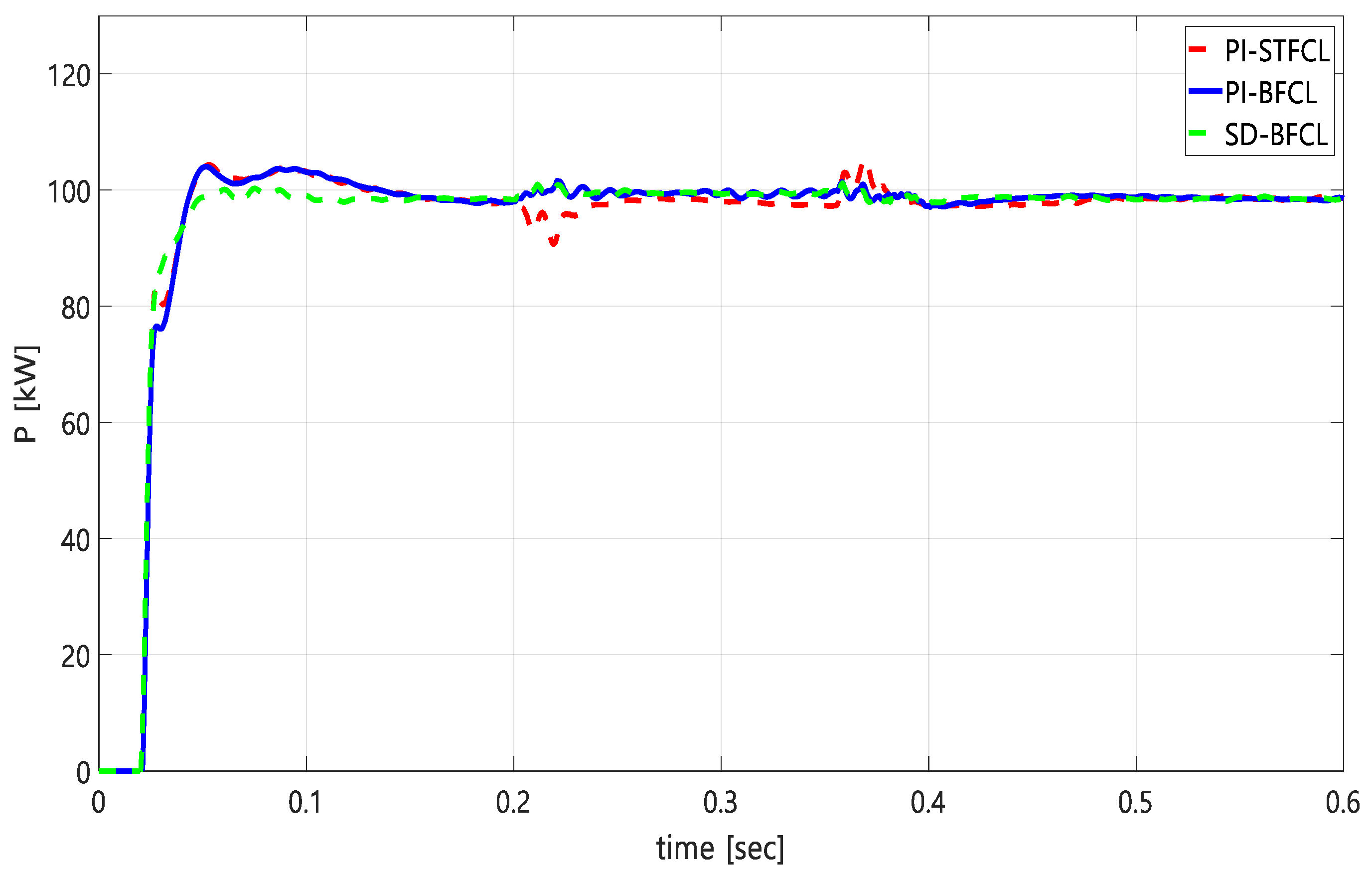
In the contemplation of the grid parameter during transient operation, the response for several proposed methods is presented for failures scenario case studies in the PCC as depicted in
Figure 10. In the period after the fault, the performance evaluation of the grid power behavior during the S-G fault shows an oscillation-free and steady power response with SD along with the BFCL except for small fluctuations in the power value, which is negligible, at fault occurring and clearing the fault. This condition occurs with similar explanation as the DC link voltage. The exceptional improvement is also depicted in the grid active power side of the system for SD alongside the BFCL. The smooth operation of the DC link voltage delivers a great performance in the grid active power side. Furthermore, the poor performance of the conventional controller, e.g., PI + STFCL, could be described with the same explanation, which is also reflected in the DC link voltage result. Moreover, the response of the PI controller with the STFCL method shows oscillation and a spike in the case of clearing the fault. This occurs due to characteristic of circuitry protection, which works based on fault current limiter switching (SW). The switching (SW) operation is bypassed at the normal condition and disconnected during the abnormal condition. In addition, the oscillation is inevitable in this controller. Meanwhile, the proposed algorithm steepest descent method with the BFCL method shows lower vibration or oscillations, and a spike cannot be obtained. Considering the reactive components in the PCC, the proposed SD controller with the BFCL strategy combination provides a smooth and spike-free response. Based on these results, the proposed method with BFCL strategies compared to reference values for grid power would be the best of the proposed FRT strategies.
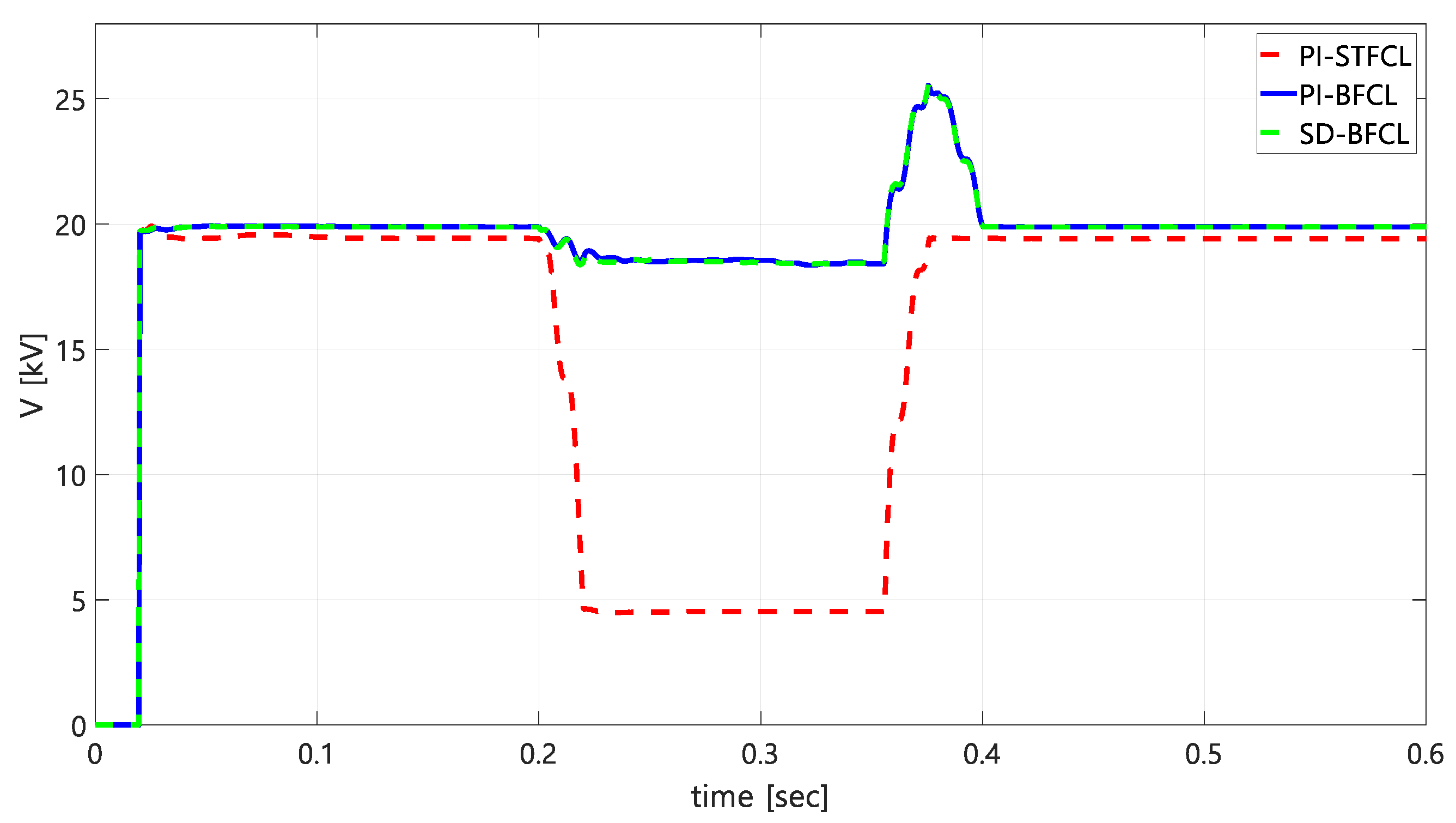
As illustrated in
Figure 11, the crucial parameter for FRT strategy, i.e., grid voltage situations, describes in detail the performance of different control methods. As mentioned in the previous section, several countries announced the grid code to maintain voltage during abnormal operation. Moreover, the LVRT description could be explained from the figure. However, the response of the PI controller with the STFCL method shows the wide decrease in voltage during the fault. The reason could be described based on the switching situation of circuitry protection in the system.
During the abnormal condition, the switch (SW) remains off. In addition, the wide decrease in the voltage value could be investigated using the grid value prior to the fault condition, which is that PI + STFCL has a wide reduction of voltage of approximately 75%. According to this value, using this method could bring tremendous risk to the grid voltage stability standard. Meanwhile, the conventional algorithm and proposed algorithm (i.e., PI and steepest descent method) with the BFCL method show that a smooth operation and wide decrease in voltage value cannot be obtained. However, there are some voltage spikes after the fault condition, which is the value of the voltage spike around 25%. Considering the reactive components in the PCC, the proposed SD controller with the BFCL strategy combination provides a smooth operation. According to these results, the proposed method (i.e., BFCL along with PI and SD) compared to the reference value for the grid power would be the best of the proposed FRT strategies.
In addition, three control measurements in the grid voltage parameter are calculated, which consist of IAE, ISE and ITAE. These measurements provide an exact and accurate distinction in contrast to different controllers. The minimum value shown is the greater of efficiency. Moreover, all control measurement error value is calculated based on pu unity.
Table 2 depicts grid voltage measurement during S-G fault which shows a minimum value with the BFCL along with the SD. As shown in the table, there are significantly different values with SD + BFCL due to characteristics of the controller to maintain the grid voltage value according to normal operation during fault simulations. However, the STFCL strategy and PI have the largest value for the three parameters. As explained before, using this method for the grid voltage standard is not proper because of the reduction value of voltage during the fault condition. However, this three-parameter error table would describe the optimum method for the inverter and FRT method. According to this parameter, the proposed method (i.e., BFCL along with PI and SD) compared to reference value for grid power would be the best of the proposed FRT strategies.
4.3. Three-phase Faults to Ground Fault
The three-phases to ground is approached to determine the behavior of the power system for severe conditions. Moreover, in order to observe a DC link voltage for the grid parameter, the results in the PCC are shown in
Figure 12. The figure shows the responses of various control strategies and FRT methods to DC link voltages. In the term of severe operation, the exceptional difference of several responses in default conditions upon and after failure is depicted. Through this simulation, we could describe how important it is to validate the LVRT proposed control in severe operation. In the term after the fault, the responses of the PI + STFCL controller show that miserable transient occurs during disturbance removal. As described in
Figure 12, the oscillation value of voltage in the PI + STFCL controller during fault conditions is around 100% according to the reference voltage value prior to failure at the PCC. Furthermore, the over-voltage characteristics of the proposed methods PI + BFCL and SD + BFCL look similar over the succeeding failure at the PCC. In addition, the PI + STFCL cannot be applied for LVRT application through the simulation due to severe oscillation of voltage during fault operation, which can exceed stability standard requirements in the DC link voltage. Furthermore, the failure at the PCC slightly affects the DC link voltage value for the combination of PI and SD along with the BFCL proposed method. Similar to the single-phase fault case studies, according to reference voltage value, during fault and clearing fault conditions the proposed FRT method BFCL shows the express response compared to the STFCL method to reach an adjustable value. As expected, the proposed strategy SD + BFCL is more stable than others. Therefore, as shown in
Figure 12, the amplitude of the DC link voltage value during initial, fault and clearing fault conditions is reduced.
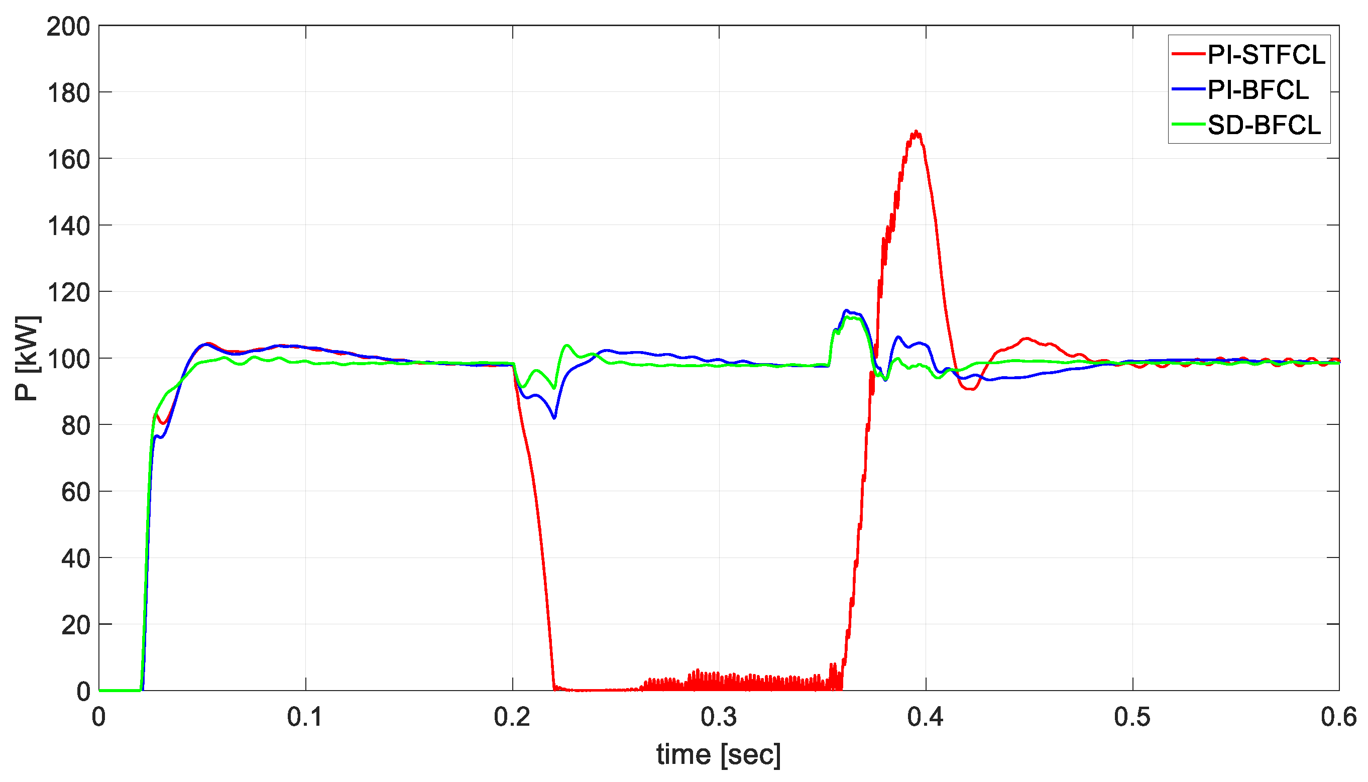
In the previous section, we already described the differences asymmetrical study would propose. In this part, the author wants to significantly describe phenomena differences for three-phase faults compared to the single-phase fault. In
Figure 13, the response for several proposed methods is presented for failures scenario case studies in the PCC. The performance evaluation of the grid power behavior during the three-phase fault shows a slight oscillation response with SD and PI along with the BFCL at the fault occurring and clearing the fault. In addition, both cases for single-phase and three-phase simulation describe the significantly different conditions for PI + STFCL. Furthermore, the response of the PI controller with the STFCL method shows the wide of oscillation and spike in the cases of fault and clearing fault. Moreover, the value of the grid active power becomes zero if the small value of oscillations is negligible during the three-phase fault condition. The series branch of
and
in parallel with the snubber capacitor act as a path for absorption of fault energy. Due to the principal working of circuitry protection, the grid active power will become zero, as well as the wide oscillation on the DC link voltage. Meanwhile, the proposed algorithm steepest descent method with the BFCL method shows lower vibration or oscillations, and the wide value of the spike in active power cannot be obtained. Considering the reactive components in the PCC, the proposed SD controller with the BFCL strategy combination provides a slightly smooth and small spike response. Based on these results, the proposed method with BFCL strategies compared to the reference value for grid power would be the best of the proposed FRT strategies.
Furthermore,
Figure 14 describes in detail the performance of different control methods in grid voltage situations during three-phase fault simulations. The response of the PI controller with the STFCL method shows a wide decrease in voltage during the fault and significantly valued oscillations. In addition, the wide decrease in voltage value could be investigated using the grid value prior to the fault condition, which is PI + STFCL having a wide reduction of voltage of approximately 90%, which is the value of reduction larger than that of the single-phase fault. According to this value, one similar to the single-phase fault condition using this method could be bring tremendous risk to the grid voltage stability standard. Meanwhile, the conventional algorithm and proposed algorithm (i.e., PI and steepest descent method) with the BFCL method show the decrease in voltage operation at around 50%, and a wide decrease in voltage value could be obtained. However, there are some voltage spikes after the fault condition, which is the value of voltage spike similar to that of the single-phase fault simulation. Considering the reactive components in the PCC, the proposed SD controller with the BFCL strategy combination provides a smooth operation. According to these results, the proposed method (i.e., BFCL along with PI and SD) compared to reference value for grid power would be the best of the proposed FRT strategies.
Furthermore, as explained in the previous section regarding three control measurements proposed in the grid voltage parameter are calculated, which consists of integral absolute error (IAE), integral square error (ISE) and integral time-weighted absolute error (ITAE). These measurements provide a precise and accurate comparison between different controllers. The minimum value is shown as the greater efficiency.
Table 3 depicts grid voltage measurement during the three-phase fault, which shows a minimum value with the BFCL along with SD, which is also similar to the single-phase fault simulation. As shown in the table, there are significantly different values with SD + BFCL due to the characteristic of the controller to maintain the grid voltage value according to normal operation during fault simulations. However, the STFCL strategy and PI have the largest value for three parameters. As explained before, using this method for the grid voltage standard is not proper because the wide reduction value of voltage is almost zero during the fault condition. However, this three-parameter error table would describe the optimum method for the inverter and FRT method. According to these parameters, the proposed method (i.e., BFCL along with PI and SD) compared to reference value for grid power would be the best of the proposed FRT strategies.
5. Conclusions
The application of this study for academia, industrialists and traders is illustrated through the existing grid code standard evaluation value. This paper emphasizes the improvement of contributions in LVRT, i.e., FRT function of two-phase and three-phase grid connection PVSs in normal conditions and asymmetric grid disturbances. The contributions of this paper are depicted through the new design of the BFCL and SD controller as the FRT strategy and inverter control to improve FRT functionality and optimize the rated removable fault current of the switch gear. Furthermore, the other advantage of BFCL topology is reducing the stress of the semiconductor device in the event of a failure.
In the case of the proposed STFCL and BFCL strategies, the response and stability of PVS during fault conditions were analyzed indiscriminately. Moreover, the proposed FRT strategy, i.e., BFCL strategy with SD controller, optimized spike behavior better than PI and STFCL during the fault condition. The power quality was improved not only on the PV side but also on the power grid side by the smooth and temporarily oscillation-free operation of voltage and current due to the SD algorithm method. The simulation results also verify performance indices evaluation, i.e., IAE, ITAE and ISE, with high efficiency and fault tolerance of the proposed strategy. For future development research, the design of inverter control will be extended by several proposed schemes such as feedback linearization, adaptive L1 and high-order adaptive SMC.


