The Impacts of COVID-19 on the Rank-Size Distribution of Regional Tourism Central Places: A Case of Guangdong-Hong Kong-Macao Greater Bay Area

Abstract

It is well known that Zipf’s rank-size law is powerful to investigate the rank-size distribution of tourist flow. Recently, widespread attention has been drawn to investigating the impacts of COVID-19 on tourism for its sustainability. However, little is known about the impacts of COVID-19 on the rank-size distribution of regional tourism central places. Taking Guangdong-Hong Kong-Macao Greater Bay Area as a research case, this article aims to examine the fractal characteristics of the rank-size distribution of regional tourism central places, revealing the impacts which COVID-19 has on the rank-size distribution of regional tourism central places. Based on the census data over the years from 2008 to 2021, this paper reveals that before COVID-19, the rank-size distribution of the tourism central places in Guangdong-Hong Kong-Macao Greater Bay Area appears monofractal, and the difference in the size of the tourism central places has a tendency to gradually decrease; in 2020, with the outbreak of COVID-19, the characteristic of the rank-size distribution shows that the original monofractal is broken into multifractal; in 2021, with COVID-19 becoming under control, the structure of tourism size distribution, changes into bifractal based on the original multifractal, showing that the rank-size distribution of tourism central places in Guangdong-Hong Kong-Macao Greater Bay Area becomes more ideal and the tourism order becomes better than the last year. The results obtained not only fill in the gap about the impacts of COVID-19 on tourism size distribution, but also contribute to the application of fractal theory to tourism size distribution. In addition, we propose some suggestions to the local governments and tourism authorities which have practical significance to tourism planning.

1. Introduction

Regional tourism resources, regional conditions, regional economic development level and other factors will cause the unbalanced development of regional tourism, so to analyze the differences in regional tourism sizes and its formation mechanism can promote the development of the backward regional tourism areas and help developed regional tourism areas to maintain their competitive advantages [1,2,3].

The COVID-19 pandemic is one of the most significant events of the 21st Century [4]. By 30 September 2020, 33,561,077 confirmed cases of COVID-19 and 1,005,004 deaths had been reported worldwide [4]. The COVID-19 pandemic has dealt a severe blow to global tourism as well as regional tourism and leisure sectors, including the hospitality subsector and its entire value chain. Since the outbreak of the COVID-19 pandemic, people have been unable to travel as usual. This severe situation leads to slow development in the tourism industry [4,5,6,7,8,9,10,11]. The coronavirus disease (COVID-19) outbreak has had a significant impact on the worldwide tourism industry and thus brought about great loss in the economy. The United Nations World Tourism Organization (UNWTO) reported that by 20 April 2020, all major tourist destinations had implemented travel restrictions in response to the COVID-19 pandemic [11]. Lockdowns in many countries, widespread travel restrictions, and airport and national border closures reduced the number of international tourist arrivals by 67 million during the first quarter of 2020. This decrease implies a loss of approximately USD 80 billion in tourism revenue, compared with the same period in 2019 [11].

Since late 2019, the COVID-19 pandemic has caused unprecedented and profound negative impacts on regional tourism in China. Take Guangdong-Hong Kong-Macao Greater Bay Area for example. In 2019, Guangdong-Hong Kong-Macao Greater Bay Area received 355,627,500 overnight tourists. However, in 2020 and 2021, due to the outbreak of COVID-19 and the subsequent travel restriction and lockdown policies launched by the authorities, the number of overnight tourists dropped quickly and amounted to 1,961,380,000 and 2,209,970,000 respectively [12,13,14].

Although the COVID-19 pandemic is impacting most companies across all industries, we still lack a deep understanding of the managerial implications of the crisis. Although there are a number of literatures involving the studying of tourism flow and the size and spatial distribution of regional tourism places [1,3,15,16,17,18,19,20,21], little is known about the impacts of COVID-19 on the rank-size distribution of regional tourism central places. Hence, we propose this question: How does the COVID-19 impact Zipf’s rank-size distribution of a regional tourism central place in China? Taking Guangdong-Hong Kong-Macao Greater Bay Area as a research case, this article aims to examine the fractal feathers of the rank-size distribution of regional tourism central places.

The contributions of this study are multifold. First, this study illustrates the definition of the fractal dimension from a natural perspective and presents a detailed proof to the assertion about the relationship between the fractal dimension D and Zipf’s dimension q (i.e., D = 1/q) in the Zipf’s rank-size law and the associated rank-size double logarithmic model, while in the existing literature this assertion is usually only offered too but its proof was not available [1,3,15,16,17,18,19,20,21,22,23,24,25].

Second, unlike previous research studies, which have presented only analysis of the rank-size distribution of regional tourism central places before the outbreak of COVID-19 [1,3,15,16,17,18,19,20,21], we further reveal the impacts that COVID-19 has on the rank-size distribution of regional tourism central places, taking Guangdong-Hong Kong-Macao Greater Bay Area as a case study.

Third, the obtained results of this article are an addition to the application of fractal theory to the field of tourism and the proposed suggestions are references for the local governments and tourism authorities to maintain the sustainability of the regional tourism.

In what follows, Section 2 will present a Theoretical Background and Literature Review; Section 3 will describe the Methodology; Section 4 will give an Empirical Analysis; and Section 5 is the last section for Discussions and Conclusions.

2. Theoretical Background and Literature Review

There are many quantitative models and methods for the study of size distribution and spatial structure [1,2,3,15,16,17,18,19,20,21,22,23,24,25,26,27,28,29,30,31,32,33,34,35,36,37,38,39,40,41,42,43,44]. At present, the quantitative research on urban size distribution or tourism size distribution is made mostly by using the Jefferson primate city law [25,44], the rank-size law, the fractal theory and so on [1,2,3,15,16,17,18,19,20,21,22,23,24,26,27,28,29,30,31,32,33,34,35,36,37,38,39,40,41,42,43]. In the study of the size distributions in tourism central places, the most commonly used is the Zipf’s rank-size law associated with fractal theory.

2.1. Guangdong-Hong Kong-Macao Greater Bay Area

Guangdong-Hong Kong-Macao Greater Bay Area consists of eleven cities including nine cities in Province Guangdong (Guangzhou, Shenzhen, Zhuhai, Foshan, Jiangmen, Dongguan, Zhongshan, Huizhou, Zhaoqing) and two special administrative regions, namely Hong Kong and Macau in China (see Figure 1). It is different from other regions in China. It is the special area with the characteristic“one country, two systems, three customs areas, four core cities”. Guangdong-Hong Kong-Macao Greater Bay Area has a total area of 56,000 square kilometers, a total population of 72.6492 million in 2019, and a GDP of CNY 11.59 trillion (RMB, the same below), whereas the total population of Guangdong Province in 2019 was 11.521 million and the GDP was CNY 10.77 trillion [12,13,14].

In 2019, the total number of tourists received nationwide was 6.155 billion, and the total tourism revenue was CNY 6.64 trillion. In 2019, Guangdong Province received 532 million overnight tourists, with a total tourism revenue of CNY 1.5158 trillion. Guangdong’s tourism revenue accounted for 22.8% of the country’s total tourism revenue, ranking first in the country, whereas Guangdong-Hong Kong-Macao Greater Bay Area received 355,627,500 overnight tourists. The total tourism revenue is CNY 1.251589 trillion, of which the total tourism revenue of the nine cities in the Pearl River Delta and Guangdong area is CNY 1.008618 trillion, which basically accounts for 80% of Guangdong’s total tourism revenue. In 2019, Hong Kong received 23.76 million overnight tourists, with a total tourism revenue of USD 32.701 billion (equivalent to RMB 232.506 billion); Macao received 18.633 million overnight visitors, and a total tourism revenue of MOP 13.42 billion (equivalent to RMB 10.465 billion) [12,13,14]. It can be seen that the comprehensive economic strength of tourism in Guangdong-Hong Kong-Macao Greater Bay Area has significant competitive advantages. Research on the size and spatial structure of the tourism central place of Guangdong-Hong Kong-Macao Greater Bay Area has strong strategic significance.

2.2. Tourism Central Places

A central place is usually defined as a settlement located in a regional center whose function is to provide consumers with certain types of products and services [45,46,47,48]. The central place theory seeks to explain the size and spacing of the human settlements, which mainly include cities and towns. In fact, geologists have long recognized that the functions of cities and towns as market centers, traffic centers and administrative centers, leads to the emergence of the hierarchical system of settlements [45]. In 1933, W. Christaller introduced the concept of a central place for the first time, which believed that the center of a region was interconnected and developed in the form of hierarchical systems and network structures [45,46,49,50,51]. Since then, people have become interested in the research of central places, and applied the theory to some related fields, including economics, sociology, urban planning, and natural geography [45].

Chen [49] pointed out that the research of central places involves a series of complexity theories, such as self-similarity, scaling and self-organization theories. The regional central places can be seen as a system with a hierarchical structure, or as a network with self-similar properties.

Hierarchical structure is a basic characteristic of a complex system, which always follows scaling laws, especially the rank-order law as well as Zipf’s law [49]. Many scholars have been interested in natural and social systems; such systems are all complex systems [50]. The most common one of hierarchical structure is the hierarchical structure of urban size. The quantitative study of urban size distribution can be traced back to the 20s of last century. From then on, some scholars in western developed countries have put forward the theory and models reflecting the law of urban size distribution. Among them, the most well-known is the Zipf’s rank-size law [54]. Later on, a number of scholars have paid great attention to the study of urban size distribution [22,23,24,27,28,29,30,31,32,33,34,35,36,37,38,39].

As it is well known that tourism plays a crucial role in the national economy in a country, a natural question is whether central place theory together with complexity theory and fractal theory as well as Zipf’s law can be used in tourism research. In fact, Jennings pointed out that chaos and complexity theory is an important theory in tourism research. The tourism system is an unstable, self-organizing, complex dynamic system ([38], p. 58), and fractal is a self-similar level with structurally complex systems, making it an ideal tool for studying chaos and complex systems [40]. People can naturally use fractal theory to study size hierarchical structures.

Since 1982, fractal theory has been widely used in various fields of natural science and social science [40]. Because fractal is a complex system with a self-similar hierarchical structure, it is an ideal tool for analyzing complexity, non-linearity, and self-organizing evolution systems, and so people may naturally study size distribution and special structure by virtue of fractal theory [22,31,32,38,40,45].

In recent years, some scholars used the above theory to study tourism, mainly involving tourism flow and the size and spatial distribution of regional tourism places [1,2,3,15,16,17,18,19,20,21,40,41,42,43].

Since the reform and opening to the world in 1978, the tourism industry in Guangdong, Hong Kong and Macao has developed rapidly, and related researches have gradually increased. Wu [2] used standard deviation, coefficient of variation, Gini coefficient, Herfindahl index and primacy to reflect the absolute difference, relative difference and balance of the income of inbound overnight tourists and inbound tourism in 11 cities in Guangdong-Hong Kong-Macao Greater Bay Area over the years from 2001 to 2016, and adopted the rank-size law to construct an inbound tourism rank-size system of Guangdong-Hong Kong-Macao Greater Bay Area, and explored the mechanism of these differences.

2.3. Fractal Theory

A fractal is a figure or complex system that satisfies certain self-similarity [40]. Fractal geometry is a science that deals with fractal sets, and it is a generalization of the traditional Euclidean geometry (i.e., integer dimension geometry) [40]. Usually, we regard the line segment as the object in the one-dimensional space. A figure in a plane is regarded as the object in the two-dimensional space, and a solid figure is regarded as an object in the three-dimensional space. So, we usually call a straight line segment, a plane figure and a solid figure one-dimensional, two-dimensional and three-dimensional, respectively. Is there a figure in nature with a non-integer dimension? In 1970s, the American mathematician B.B. Mandelbrot introduced fractal dimension to solve this problem [40]. Fractal dimension is the key element of fractal geometry [52]. Let us recall the concept of fractal dimension.

The fractal dimension originates from the analysis of geometrical figure in Euclidian spaces. Now we elaborate on this for details. As is shown in Figure 2, if a line segment with length 1 is divided equally into N line segments, then the length r of each small line segment is such that,

$$N\cdot r=1.$$

(1)

Similarly, if a square with area 1 is divided equally into N small squares, then the length r of the edge of each small square is such that,

$$N\cdot r^2=1.$$

(2)

Similarly, if a cube with volume 1 is divided equally into N small cubes, then the length r of the edge of each small cube is such that,

$$N\cdot r^3=1.$$

(3)

The power of r in the above three equations is actually the dimension of the space that the geometrical body can obtain a constant metric, so we have the following formula:

$$N\cdot r^D=1.$$

In general, for a complex geometrical body, suppose that its “volume” is C, and after dividing it into N equal parts, there is a non-integer constant D, such that,

$$N\cdot r^D=C.$$

Or alternatively,

$$N\propto r^{-D}.$$

(4)

Then, we call D the fractal dimension (i.e., self-similar dimension) [40].

Chen [49] pointed out that if the urban hierarchy system is fractal, it obeys the power law, such as the Zipf’s rank-size law.

2.4. Zipf’s Law and Rank-Size Model

2.4.1. Zipf’s Law and Rank-Size Model for Size Distribution of Cities

The tourism size is similar to city size since tourism size is usually referred to as the number of the overnight visitors [3]. In order to investigate tourism size distribution, let us recall Zipf’s rule and the rank-size model which are most commonly used in the study of city size distribution.

The rank-size law can be traced back to the early twentieth century. In 1913, when F. Auerback studied the size of a German city, by the experimental analysis he first pointed out that the relationship between the size of a city and the city’s rank in the list of the population size in a certain country obeyed a certain law [53]. He found that the size of the city with rank r is the size of the 1/r size of the primate city, that is, Pr = P₁/r, where Pr is the population of the city with rank r, and P₁ denotes the size of the primate city. This law is called the rank-size distribution rule.

In 1924, when M.L. Lotka studied the urban size of the United States, a similar law was found, which was later known as rank-size law, formally proposed by Zipf in 1949 as a theoretical model [54]. This model, also regarded as a special power law [3,27,42], is usually expressed as:

$$P_r{r}^q=P_1$$

(5)

Note that Zipf’s rank-size law is equivalent to its double-logarithmic format, as follows:

$$\ln P_r=\ln P_1-q\ln r$$

(6)

Equation (6) shows that there is a linear relationship between the logarithm of city size and the logarithm of the corresponding rank, where q is called regression slope or Zipf dimension. When the q value is close to 1, it indicates that the city size distribution is approaching to the Zipf ideal state; when the q value is more than 1, it indicates that the city size distribution is more concentrated, the big cities are very prominent whereas the small and medium cities are not developed; when the q value is less than 1, it indicates that the city size distribution is relatively scattered, the big cities are not prominent, whereas the medium and small cities are more developed.

2.4.2. Zipf’s Law and Rank-Size Model for Size Distribution of Regional Tourism Central Places

Many scholars investigate tourism rank-size distribution by utilizing Zipf’s rank-size law and its double-logarithmic format [1,3,16,18,19]. Among them, Lan, Koo and Wu point out that the power law could be used to describe the rank-size relationship of tourism destinations where the tourism size refers to the number of overnight visitors [3].

In this section, we will introduce Zipf’s rank-size distribution model of regional tourism central places, and use the fractal theory associated with the rank-size rule to reveal the relationship between Zipf’s dimension and fractal dimension in Zipf’s rank-size distribution model.

In Equation (6), we take the value of Pr as the number of the overnight visitors received by the tourism central place with the rank r. The specific methods are as follows: Suppose that the number of the regional tourism central places in the regional tourism system discussed is n. First, collect the initial basic data, i.e., the number of tourists received by each tourism central place in the regional tourism system, which is regarded as the size of the tourism central place. Second, arrange these $n$ numbers from large to small, so as to obtain n ordered numbers, writing Pr (r = 1, 2, …, n), where $P_1\ge P_2\ge \dots \ge P_n$. If Zipf’s urban rank-size distribution formula (5) is suitable for size distribution of the regional tourism central places, then we have

$$P_r=P_1{r}^{-q}$$

(7)

where P_r is regarded as the size of the tourism central place with rank r; P₁ refers to the number of tourists received by the primate tourism central place; and q denotes Zipf dimension. By means of the definition of fractal dimension and the Equation (7), we can prove the relationship between fractal dimension D and Zipf’s dimension q is such that D = 1/q (see Appendix A).

In order to compute the value of q, taking the logarithm of Equation (7), we have

$$\ln P_r=\ln P_1-q\ln r$$

(8)

After taking r = 1, 2, …, n, all the pairs of data (lnr, lnP(r)) are plotted on the double logarithmic coordinate plots, and the linear regression analysis is carried out to get the fitting line and the linear regression equation. The Zipf’s dimension is derived from the regression equation, and then the value of fractal dimension can be obtained by the formula D = 1/q. When the scatter points fit the straight line well, it shows that the distribution of tourism size in this region conforms to Zipf’s rank-size law and has the fractal characteristics.

The fractal dimension D has the following practical significance in the context of regional tourism central places [1].

When the fractal dimension is such that D = 1, it shows that $P_1=n{P}_n$, which indicates that the ratio of the size of the primate tourism central place to that of the tourism central place with the smallest size is the number of tourism central places in the whole tourism system in the region. The regional distribution of the visitors in this area is moderate, and the size hierarchy of the tourism central places is reasonable.

When the fractal dimension is such that D > 1, it shows that the size distribution of the tourism central places in this area is relatively concentrated, its distribution equilibrium degree is high, the number of tourism central places with a medium tourism size (that is, the tourism central places ranked in the middle) is relatively more, the number of tourists received by the primate tourism central place is relatively small, and the monopoly position is weak. When fractal dimension is such that D < 1, it shows that the size distribution of the tourism central places in this area is relatively scattered. The degree of distribution balance is poor, the primate tourism central place received a lot of tourists, the monopoly position is obvious, the first degree index is often higher, and the distinction degree of tourism sizes of any two tourism central places is very obvious.

3. Methodology

3.1. Linear Regression Analysis

We will conduct empirical Analysis by means of software Excel as well as SPSS (Statistical Package for the Social Science) 25.0 to carry out the linear regression to investigate rank-size distribution. Taking lnP(r) as the ordinate and lnr as the abscissa, by conducting the simple linear regression analysis without any controls, we get the fitting lines for the points (lnr, lnP(r)) based on the collecting data, which are the so-called double logarithmic plots of the size distribution of tourism central places in Guangdong-Hong Kong-Macao Greater Bay Area. In addition, we also do the White heteroskedasiticity test and estimate the robust standard errors to heteroskedasiticity.

3.2. The Data Collection

The total number of overnight tourists received in 11 prefecture-level cities in Guangdong-Hong Kong-Macao Greater Bay Area from 2008 to 2021 is selected as the basic data used in this study. These data come from the statistics information website of Guangdong Province [12], the website of the Hong Kong Tourism Board (see [13]), and the website of the Macao Special Administrative Region Tourism Bureau (see [14]). The 11 tourism central places in the district receive the total number of overnight tourists (see

Table 1. Tourist reception size of the tourism central places in Guangdong-Hong Kong-Macao Greater Bay Area. (2008–2021, Unit: 10,000 person time).

	2008	2009	2010	2011	2012	2013	2014	2015	2016	2017	2018	2019	2020	2021
GZ	3528.7	3975.5	4506.4	4595	4809.6	5042	5330	5658	5940.6	6275.6	6532.6	6773.2	4182.6	4307.7
SZ	2659.3	2840.1	3285.3	3732.5	4147	4567	4991	5375	5695.7	6022	6407.9	6718	4968.8	6364
ZH	808.2	1208.7	1380.5	1535.7	1596.4	1572	1809	1924	2226.4	2288.6	2640.4	2182.5	960.4	1004.7
FS	802.4	835.9	866.6	980.7	1045.2	1119	1182	1253	1351	1497.8	1695.3	1933	1757.2	1596.9
HZ	807.7	943.1	1074	1189	1312.8	1502	1655.5	2076.8	2033	2239	2440.6	2992.9	1296.7	1366.6
DG	1872	2037	2251	2615.5	2743.8	2826	2791	3199.1	3792	4141.9	4433.9	4456.6	3876.5	4553.6
ZS	528.1	551.9	587.9	665.3	800.3	861.4	902.2	986.6	1117.8	1333.5	1412.2	1496.3	817.7	839.7
JM	839.4	861.9	991	1161.7	1284.7	1410	1602	1548	2000.6	2259	2722.7	3337	728.9	777.0
ZQ	710.8	840.5	1055.7	1264	1392.2	1388	1112.4	1127.7	1236	1329.8	1353	1434	501.7	618.1
HK	1682	1693	2008	2232	2377	2567	2777	2669	2655	2788	2926	2376	135.9	8.9
MC	1061	1040.2	1192.6	1292.5	1357.7	1427	1456.5	1430.8	1570	1725.5	1849.3	1863.3	387.4	662.5

).

4. Empirical Analysis

4.1. Results for Simple Linear Regression Analysis without Any Controls

In this subsection, we will conduct simple linear regression analysis without any controls to investigate the fractal characteristics of size distribution of tourism central places in Guangdong-Hong Kong-Macao Greater Bay Area.

According to the log-log rank-size model (8) for size distribution of regional tourism central plases, based on the data in Table 1, we need to draw the double logarithmic plots of the rank-size distribution of tourism central places in Guangdong-Hong Kong-Macao Greater Bay Area over the years 2008–2021, and then identify whether there exists monofractal, bifractal or multifractal in the double logarithmic plots. At last, we analyze the characteristics of the size distribution of tourism central places in Guangdong-Hong Kong-Macao Greater Bay Area.

In order to describe the detailed process, we take the data from the year 2019 as an example. According to the size of the total number of overnight tourists received in 2019 from each of the 11 tourism central places in Guangdong-Hong Kong-Macao Greater Bay Area, we obtain the table by showing the rank size of tourism central places in Guangdong Province in 2019 (see

Table 2. Rank-size of tourism central places in Guangdong-Hong Kong-Macao Greater Bay Area (2019).

Tourism Central Places	Rank r	Tourist Reception Size P(r) (10,000 Person Time)	Tourism Central Places	Rank r	Tourist Reception Size P(r) (10,000 Person Time)
GZ	1	6773.2	ZH	7	2182.5
SZ	2	6718.0	FS	8	1933.0
DG	3	4456.6	MC	9	1863.3
JM	4	3337.0	ZS	10	1496.3
HZ	5	2992.9	ZQ	11	1434.0
HK	6	2376.0

). Since the power function relation is equivalent to the logarithmic linear relation, once the 11 points (lnr, lnP(r)) (where P(r) denotes the size of the tourism central place ranked r) in the double logarithmic plot fit a straight line well, it shows that the size distribution of tourism central places in Guangdong-Hong Kong-Macao Greater Bay Area in 2019 abides by Zipf’s rank-size rule and has the typical fractal characteristic [18,21].

Taking lnP(r) as the ordinate and lnr as the abscissa, and using the data indicated in Table 2, we can make the scatter plot, and then the linear regression is carried out via Excel to obtain the double logarithmic figure of the size distribution of Guangdong tourism central places in 2019 (see Figure 3).

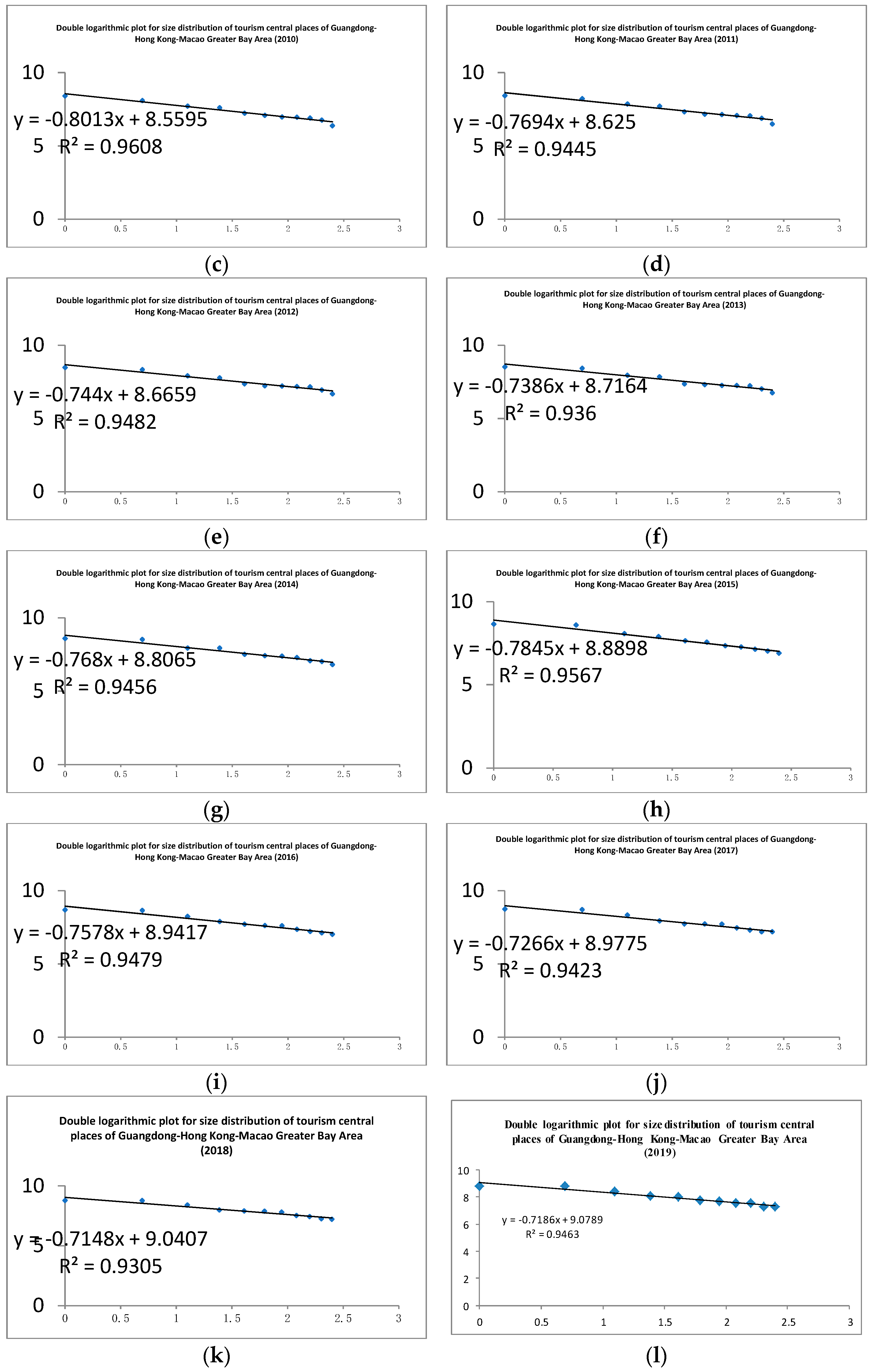
Similarly, we can also get double logarithmic plots of the size distribution of tourism central places in the other years. All the double logarithmic plots of the size distribution of tourism central places in Guangdong-Hong Kong-Macao Greater Bay Area in the years 2008–2021 are as shown in Figure 4.

According to Figure 4, the regression equations, Zipf’s dimensions q and fractal dimensions D for the size distribution of 11 tourism central places in Guangdong-Hong Kong-Macao Greater Bay Area over the years 2008–2021 are obtained. The results of the regression analysis are shown in

Table 3. Results of regression analysis for the size of tourism central places in Guangdong-Hong Kong-Macao Greater Bay Area (2008–2021).

Years	Regression Equations	q	R2	D
2008	y = −0.7934x + 8.320	0.7934	0.9544	1.2604
2009	y = −0.7900x + 8.414	0.7900	0.969	1.2658
2010	y = −0.8013x + 8.560	0.8013	0.9608	1.2480
2011	y = −0.7684x + 8.625	0.7684	0.9445	1.2997
2012	y = −0.7440x + 8.666	0.7440	0.9482	1.3441
2013	y = −0.7396x + 8.716	0.7396	0.936	1.3539
2014	y = −0.7680x + 8.807	0.7680	0.9456	1.3021
2015	y = −0.7845x + 8.890	0.7845	0.9567	1.2474
2016	y = −0.7578x + 8.942	0.7578	0.9479	1.3196
2017	y = −0.7266x + 8.978	0.7266	0.9423	1.3763
2018	y = −0.7148x + 9.041	0.7148	0.9305	1.3990
2019	y = −0.7186x + 9.079	0.7186	0.9463	1.3916
2020	y = −1.3600x + 9.164	1.3600	0.8380	0.7353
2021	y = −1.7470x + 9.648	1.7470	0.5470	0.5734

.

4.2. Heteroskedasticity Test and Parameter Estimates with Robust Standard Errors to Heteroskedasticity

4.2.1. Heteroskedasticity Test

The linear regression model is commonly used by practitioners in empirical analyses in fields such as chemistry, economics, finance, medicine, physics, among others. It is well known that when the assumptions of the linear regression model are correct, ordinary least squares (OLS) provides efficient and unbiased estimates of the parameters. An assumption that is frequently violated is that of homoskedasticity, that is, the assumption that all errors share the same variance. Instead, heteroskedasticity occurs when the variance of the errors varies across observations. SPSS 25.0 provides four types of method for completing heteroskedasticity tests, namely the Modified Breusch–Pagan test, F test, Breusch–Pagan test and White test. We utilize White test to do heteroskedasticity tests since it is suitable for the case of either linear models or nonlinear models [55]. Based on the collecting data in this study, the results of the White tests for heteroskedasticity are shown in

Table 4. The results of White tests for heteroskedasticity ^a,b,c.

Year	Chi-Square	Freedom	Sig.	Significance Level	Significance Result	Heteroskedasticity
2008	7.070	2	0.029	0.05	<0.05	Yes
2009	3.821	2	0.148	0.05	>0.05	No
2010	2.715	2	0.257	0.05	>0.05	No
2011	3.242	2	0.198	0.05	>0.05	No
2012	4.328	2	0.115	0.05	>0.05	No
2013	3.179	2	0.204	0.05	>0.05	No
2014	6.088	2	0.048	0.05	<0.05	Yes
2015	8.657	2	0.013	0.05	<0.05	Yes
2016	9.046	2	0.011	0.05	<0.05	Yes
2017	8.229	2	0.016	0.05	<0.05	Yes
2018	8.817	2	0.012	0.05	<0.05	Yes
2019	9.605	2	0.008	0.05	<0.05	Yes
2020	2.851	2	0.240	0.05	>0.05	No
2021	3.845	2	0.243	0.05	>0.05	No

^a. Dependent variables: Y1, Y2, Y3, Y4, Y5, Y6, Y7, Y8, Y9, Y10, Y11, Y12, Y13, Y14. ^b. Test the null hypothesis that the error variance does not depend on the value of the independent variable. ^c. Design: Intercept + X + X × X, where X denotes the predictor variable.

.

As is indicated in Table 4, for the collecting data in the year 2008 and the six years from 2014 to 2019, since the significance results are such that Sig. is smaller than 0.05, we assert that heteroskedasticity occurs. Hence, it is necessary to use a practical method that corrects for heteroscedasticity for the present data analysis.

4.2.2. Parameter Estimates with Robust Standard Errors to Heteroskedasticity

Since the errors are heteroskedastic, the OLS estimator remains unbiased, but becomes inefficient. More importantly, the usual procedures for hypothesis testing are no longer appropriate. In order to assure the coefficient estimates are efficient and unbiased, we need effective and practicable methods that correct for heteroskedasticity for the present data analysis. It is currently common to use standard errors and associated confidence intervals that are robust to the presence of heteroskedasticity. The most widely used form of the robust, heteroskedasticity-consistent standard errors is that associated with the work of White [55]. It turns out to use tests based on a heteroskedasticity consistent covariance matrix, hereafter HCCM. Theoretically, use of the HCCM allows a researcher to easily avoid the adverse effects of heteroskedasticity even when nothing is known about the form of heteroskedasticity. Nonetheless, White’s estimator [55], which we shall denote by HC0, is typically quite biased and can deliver unreliable testing inference in small to moderately large samples, more so under leveraged data. Several alternatives were proposed in the literature, such as the HC1 [56], HC2 [57], HC3 [58], and HC4 [59] estimators. Scholars suggest that when the number of sample N is no more than 250, the HCCM known as HC3 should be used [58].

Hence, in this subsection, data analysts should correct for heteroskedasticity using HC3 due to the small number of samples. The results of the parameter estimates with robust standard errors to heteroskedasticity by using HC3 are shown in

Table 5. Results of parameter estimates with robust standard errors to heteroskedasticity ^a (Year: 2008).

Parameter	Coefficients	Robust Standard Error b	t	Sig.	95% Confidence Intervals
					Lower Limit	Upper Limit
Intercept	8.320	0.349	23.716	0.000	7.479	9.056
X	−0.7934	0.182	−4.197	0.002	−1.175	−0.352

^a. Dependent variable: Y1; ^b. Method: HC3.

,

Table 6. Parameter estimates with robust standard errors to heteroskedasticity ^a (Year: 2009).

Parameter	Coefficients	Robust Standard Error b	t	Sig.	95% Confidence Intervals
					Lower Limit	Upper Limit
Intercept	8.414	0.164	51.216	0.000	8.042	8.785
X	−0.7900	0.093	−8.495	0.000	−1.000	−0.580

^a. Dependent variable: Y2; ^b. Method: HC3.

,

Table 7. Parameter estimates with robust standard errors to heteroskedasticity ^a (Year: 2010).

Parameter	Coefficients	Robust Standard Error b	t	Sig.	95% Confidence Intervals
					Lower Limit	Upper Limit
Intercept	8.560	0.190	45.070	0.000	8.130	8.898
X	−0.8013	0.108	−7.444	0.000	−1.045	−0.558

^a. Dependent variable: Y3; ^b. Method: HC3.

,

Table 8. Parameter estimates with robust standard errors to heteroskedasticity ^a (Year: 2011).

Parameter	Coefficients	Robust Standard Error b	t	Sig.	95% Confidence Intervals
					Lower Limit	Upper Limit
Intercept	8.625	0.248	34.802	0.000	8.064	9.186
X	−0.7684	0.137	−5.632	0.000	−1.079	−0.460

^a. Dependent variable: Y4; ^b. Method: HC3.

,

Table 9. Parameter estimates with robust standard errors to heteroskedasticity ^a (Year: 2012).

Parameter	Coefficients	Robust Standard Error b	t	Sig.	95% Confidence Intervals
					Lower Limit	Upper Limit
Intercept	8.666	0.246	35.291	0.000	8.110	9.221
X	−0.7440	0.131	−5.669	0.000	−1.041	−0.447

^a. Dependent variable: Y5; ^b. Method: HC3.

,

Table 10. Parameter estimates with robust standard errors to heteroskedasticity ^a (Year: 2013).

Parameter	Coefficients	Robust Standard Error b	t	Sig.	95% Confidence Intervals
					Lower Limit	Upper Limit
Intercept	8.716	0.256	34.010	0.000	8.137	9.296
X	−0.7396	0.136	−5.443	0.000	−1.046	−0.432

^a. Dependent variable: Y6; ^b. Method: HC3.

,

Table 11. Parameter estimates with robust standard errors to heteroskedasticity ^a (Year: 2014).

Parameter	Coefficients	Robust Standard Error b	t	Sig.	95% Confidence Intervals
					Lower Limit	Upper Limit
Intercept	8.807	0.297	29.685	0.000	8.135	9.478
X	−0.7680	0.155	−4.959	0.000	−1.118	−0.418

^a. Dependent variable: Y7; ^b. Method: HC3.

,

Table 12. Parameter estimates with robust standard errors to heteroskedasticity ^a (Year: 2015).

Parameter	Coefficients	Robust Standard Error b	t	Sig.	95% Confidence Intervals
					Lower Limit	Upper Limit
Intercept	8.890	0.322	27.634	0.000	8.162	9.618
X	−0.7845	0.167	−4.685	0.001	−1.163	−0.406

^a. Dependent variable: Y8; ^b. Method: HC3.

,

Table 13. Parameter estimates with robust standard errors to heteroskedasticity ^a (Year: 2016).

Parameter	Coefficients	Robust Standard Error b	t	Sig.	95% Confidence Intervals
					Lower Limit	Upper Limit
Intercept	8.942	0.325	27.532	0.000	8.207	9.676
X	−0.7578	0.169	−4.473	0.002	−1.141	−0.375

^a. Dependent variable: Y9; ^b. Method: HC3.

,

Table 14. Parameter estimates with robust standard errors to heteroskedasticity ^a (Year: 2017).

Parameter	Coefficients	Robust Standard Error b	t	Sig.	95% Confidence Intervals
					Lower Limit	Upper Limit
Intercept	8.978	0.303	29.584	0.000	8.291	9.664
X	−0.7266	0.158	−4.607	0.001	−1.083	−0.370

^a. Dependent variable: Y10; ^b. Method: HC3.

,

Table 15. Parameter estimates with robust standard errors to heteroskedasticity ^a (Year: 2018).

Parameter	Coefficients	Robust Standard Error b	t	Sig.	95% Confidence Intervals
					Lower Limit	Upper Limit
Intercept	89.041	0.329	27.502	0.000	8.297	9.784
X	−0.7148	0.173	−4.144	0.003	−1.105	−0.325

^a. Dependent variable: Y11; ^b. Method: HC3.

and

Table 16. Parameter estimates with robust standard errors to heteroskedasticity ^a (Year: 2019).

Parameter	Coefficients	Robust Standard Error b	t	Sig.	95% Confidence Intervals
					Lower Limit	Upper Limit
Intercept	9.079	0.331	27.405	0.000	8.329	9.828
X	−0.7186	0.173	−4.163	0.002	−1.109	−0.328

^a. Dependent variable: Y12; ^b. Method: HC3.

.

As is shown in Table 5, Table 6, Table 7, Table 8, Table 9, Table 10, Table 11, Table 12, Table 13, Table 14, Table 15 and Table 16 compared to the original simple regression analysis results, since the regression coefficients are unchangeable, the Zipf’s dimensions and fractal dimensions are also as the same as before. However, the significance is usually changeable. Especially, the robust standard errors are quite different from the initial standard errors appearing in the simple regression analysis without any controls, which assures the precision of the estimates completely.

According to the results of the regression analysis in Table 3, the correlation coefficients of the regression analysis for the years 2020 and 2021 are 0.8380 and 0.5470, respectively, relatively small and all below 0.84, which reveals that the data for these two years are not suitable for linear regression, so we need not make further parameter estimates with robust standard errors to heteroskedasticity.

4.3. Fractal Analysis on the Size Distribution of Regional Tourism Central Places

It can be clearly seen from Table 3 that the change in the fractal dimension D value over the years. During the 14 years from 2008 to 2021, the fractal dimension D of the size distribution of tourism central places in Guangdong-Hong Kong-Macao Greater Bay Area fluctuated to a certain extent, and gradually increased from 2008 to 2019 from the general trend; because of the influences of the new crown epidemic on tourism, the fractal dimension D dropped abruptly from 1.3916 in 2019 to 0.7353 in 2020, and then continued to decrease to 0.5723 in 2021.

According to the change in the fractal dimension D of the size distribution of the tourism central places in the Guangdong-Hong Kong-Macao Greater Bay Area (see Table 3) and the scatter point distribution of the double logarithmic plots over the years (see Figure 4), the development process of the size distribution of the tourism central places in the Guangdong-Hong Kong-Macao Greater Bay Area from 2008 to 2021 can be recognized as three stages:

The first stage (from 2008 to 2019): In this stage, the fractal dimension D value of the tourism size distribution generally increased but occasionally fluctuated, that is, although the fractal dimension D of the tourism size distribution decreased slightly in 2010, 2014, 2015 and 2019, but in general it was in a trend of gradual increase, which shows that the tourism size of small- and medium-scale tourism central places is faster than that of large-scale tourism central places, such as Guangzhou and Shenzhen. For example, the size of tourism in Guangzhou in 2019 was 67.732 million, less than double the 35.278 million in 2008, whereas the size of tourism in mid-sized cities such as Huizhou, Dongguan, Zhongshan, Jiangmen in 2019 was so high that they were almost four times of that in 2008. For example, the size of tourism of Jiangmen was 33.37 million person-times in 2019; it was 3.98 times of that (8.394 million person-times) in 2008. There is only one scale-free area at this stage, and 11 tourist centers are all on the scale-free area, indicating that the rank-size distribution of the tourism central places in Guangdong-Hong Kong-Macao Greater Bay Area has a kind of monofractal structure [51].

The second stage (2020): Due to the impact of COVID-19, global tourism has been hit hard, and the tourism industry in Guangdong-Hong Kong-Macao Greater Bay Area has been severely influenced.

As can be seen from Figure 4m, the rank-size distribution of tourism central places in Guangdong-Hong Kong-Macao Greater Bay Area in 2020 has three scale-free areas. The regression analysis results showing these three scale-free areas are shown in Figure 5.

It can be seen from the scatter diagram in Figure 4m that the 3 points ranked 1, 2 and 3 are located in the first scale-free area; the 5 points ranked 4, 5, 6, 7 and 8 are located in the second scale-free area; the 3 points ranked 8, 9 and 10 are located in the third scale-free area; and the point ranked 11 is not located in any scale-free area (see Figure 5). If the data for all these 11 points are used to conduct regression analysis as a whole, the regression coefficient is determined to be 0.9647, and the fractal dimension D is 1.5678. If this data fitting is divided into the above three segments, then the regression coefficient and the fractal dimension are changeable accordingly. In fact, if the regression analysis is conducted only for the 3 points ranked 1, 2 and 3, then the regression coefficient is determined to be 0.9951, and the fractal dimension D is 4.3783; if the regression analysis is conducted only for the 5 points ranked 4, 5, 6, 7 and 8, then the regression coefficient is determined to be 0.9889, and the fractal dimension D is 0.7686; if the regression analysis is conducted only for the 3 points ranked 8, 9 and 10, then the regression coefficient is determined to be 0.9948, and the fractal dimension D is 0.3522 (see Figure 5 and

Table 17. Multi-index applied in analysis of the size of tourism central places in Guangdong-Hong Kong-Macao Greater Bay Area (2020–2021).

Years	Scale-Free Areas	Domain for Scale-Free Areas	Regression Equations	Zipf Dimension q	Fractal Dimension D	R2
2020	1st scale-free areas	K = 1–3	y = −0.2264x + 8.5072	0.2284	4.3783	0.9951
	2nd scale-free areas	K = 4–8	y = −1.301x + 9.254	1.301	0.7686	0.9889
	3rd scale-free areas	K = 8–10	y = −2.8392x + 12.483	2.8392	0.3522	0.9948
2021	1st scale-free areas	K = 1–3	y = −0.7369x + 8.7372	0.369	2.710	0.9427
	2nd scale-free areas	K = 4–10	y = −1.0859x + 8.8965	1.0859	0.9443	0.9860

).

Based on facts above we see the regression coefficients (namely, 0.9951, 0.9889 and 0.9948) of the three data fitting are significantly higher than the regression coefficient (namely, 0.9647) of the overall fitting, and the fractal dimension values (namely, 4.3783, 0.7686 and 0.3522) for the three segments are significantly different. Hence, the rank-size distribution of the tourism central places of Guangdong-Hong Kong-Macao Greater Bay Area has a multifractal structure.

According to the results of the regression analysis shown in Figure 5 and Table 4, Guangzhou, Shenzhen and Dongguan, which are the top three central places in terms of tourism size, constitute the first scale-free area; the second scale-free area consists of the five central places ranked 4–8 in terms of tourism size, namely, Foshan, Huizhou, Zhuhai, Zhongshan, and Jiangmen; the third scale-free area consists of the three central places ranked 8–10 in tourism size, namely, Jiangmen, Zhaoqing, and Macau, of which Jiangmen, ranked 8, is located at the intersection of the two scale-free areas, whereas Hong Kong is not located in any scale-free area due to its very small tourism size. It can be also seen from Table 4 that the fractal dimension D of the first scale-free area is 4.3783, which is significantly higher than that of 1.3919 of the first one in 2019, indicating that the difference of the tourism sizes of the three central places in the first scale-free area, Guangzhou, Shenzhen and Dongguan, is still shrinking since the fractal dimension is larger than 1. Moreover, the fractal dimension D of the second scale-free area is 0.7686 less than 1, which indicates that the difference of the tourism sizes of the five central places included in the second scale-free area (i.e., Foshan, Huizhou, Zhuhai, Zhongshan and Jiangmen) is large. In addition, the fractal dimension D of the third scale-free area is 0.3522, less than 1, and it is very small, which reveals that the difference in the tourism sizes of the three central places included in the third scale-free area (i.e., Jiangmen, Zhaoqing, and Macao) that are included in the scale-free area is very large.

As is shown in Figure 5, Hong Kong, the size of which is smallest, did not fall into any scale-free area; it is in a relatively independent position. Therefore, the size distribution of tourism central places in Guangdong-Hong Kong-Macao Greater Bay Area in 2020 has a multifractal structure [51].

The third stage (2021): As can be seen from Figure 6, two scale-free areas existed in the size distribution of tourism central places in Guangdong-Hong Kong-Macao Greater Bay Area in 2021.

Among these eleven tourism central places, the top three central places in terms of tourism size are Guangzhou, Shenzhen and Dongguan and they are located in the first scale-free area. Moreover, Foshan, Huizhou, Zhuhai, Zhongshan, Jiangmen, Macao, and Zhaoqing, which rank 4–10 in terms of tourism size, are located in the second scale-free area, whereas Hong Kong, the size of which ranks last, is not within any scale-free area because of its too small tourism size (noting that Hong Kong has a tourism size of 89,000 person-times due to the severe impact of COVID-19 epidemic, which is 1.44% of the 6.181 million person-times in Zhaoqing which ranks 10 in terms of tourism size). It can be seen from Table 5 that the three central places located in the first scale-free area are consistent with those in 2020, but the fractal dimension D is reduced from 4.3783 in 2020 to 2.710 in 2021, which shows that the difference in tourism sizes of the three centers, namely, Guangzhou, Shenzhen and Dongguan, in the first scale-free area increased after one year, and the trend was along the direction from being greater than 1 to approaching to 1. For the first scale-free area, the regression coefficient was 0.9427, which indicated that the data fit was good and the conclusion was reliable. The seven central places (i.e., Foshan, Huizhou, Zhuhai, Zhongshan, Jiangmen, Macao and Zhaoqing) included in the second scale-free area in 2021 are exactly the same as the total central places located in the first and second scale-free area in 2020, and the fractal dimension D (0.9443) is larger than each of the fractal dimensions D of the first scale-free area and the second scale-free area in 2020 (D is 0.7686 and 0.3522 respectively), which shows that the difference of the tourism size of the seven central places in the second scale-free area becomes smaller after one year, and the trend is along the direction from being less than 1 to approaching to 1, and the regression coefficient is greater than 0.98, indicating that the data fits well and the conclusion is reliable.

Based on the above arguments, we assert that the size distribution of tourism central places in Guangdong-Hong Kong-Macao Greater Bay Area in 2021 has a kind of bifractal structure.

5. Discussions and Conclusions

Based on the tourism data on the overnight tourists from eleven tourism central places in Guangdong-Hong Kong-Macao Greater Bay Area over the years from 2008 to 2021, and the results of rank-size double-logarithmic regression analysis, we can draw the following conclusions:

Firstly, the rank-size distribution of Guangdong-Hong Kong-Macao Greater Bay Area had a characteristic of monofractal before COVID-19. From 2008 to 2019, according to the results of regression analysis for the data, the correlation coefficients are relatively large, all above 0.93, so we are sure the 11 points appear to be located almost in the same straight line, indicating that the rank-size distribution of Guangdong-Hong Kong-Macao Greater Bay Area tourism central places had the feature of typical monofractal before COVID-19.

Secondly, the rank-size distribution of Guangdong-Hong Kong-Macao Greater Bay Area had a characteristic of multifractal in the first year after COVID-19. Since the outbreak of the new crown epidemic at the end of 2019, the structure of rank-size distribution in tourism central places in the Guangdong-Hong Kong-Macao Greater Bay Area has degraded from the original mono-fractal to a kind of local fractal, and so a multifractal structure appeared in 2020 (owing three scale-free areas), making the structure of size distribution of regional tourism central places more complex, and changing from a monofractal before the epidemic to three subfractals, together with Hong Kong as a relatively independent “isolated point”.

Thirdly, the rank-size distribution of Guangdong-Hong Kong-Macao Greater Bay Area has a characteristic of bifractal in the second year after COVID-19. In fact, the structure of rank-size distribution in 2021 became bi-fractal although the original was multifractal, indicating that the tourism order in the tourism central places in Guangdong-Hong Kong-Macao Greater Bay Area was further improved in 2021, which shows that the effective measures for epidemic prevention and control in the years 2020 and 2021 have had a positive effect on the tourism development of the Guangdong-Hong Kong-Macao Greater Bay Area.

In order to speed up and improve the construction of a tourism central place in Guangdong-Hong Kong-Macao Greater Bay Area, we put forward the following suggestions, which may help the tourism authorities to conduct tourism planning for sustainability of tourism after the outbreak of COVID-19.

Firstly, persist in classification guidance and improve the rationality of the difference of the size. For Guangzhou, which ranks first in the size of tourism, its comprehensive tourism strength ranks in the forefront of the regional tourism central places. It should focus on developing its location and transportation advantages and innovative advantages to improve the quality of tourism development, give full play to the leading role of the first rank tourism central place, continuously strengthen the first position in the size structure of the province’s tourism destinations, and improve the hierarchical structure of size. For Shenzhen, which ranks second, due to the rapid development of tourism in recent years, the size of tourism has been close to the first city, and the current development momentum needs to be maintained in the future.

For medium-size cities such as Dongguan, Foshan and Jiangmen, etc., although tourism development continues to heat up, there is still a big gap with the top two central tourist destinations. The focus should be on promoting resource integration, regional tourism interaction, and regional harmonious development. For the smallest size city, Hong Kong, the local government must take effective measures to control COVID-19 and restore the economic and social order in order to promote the development of the tourism industry.

Next, we should vigorously develop the construction of the tourism infrastructure, optimize the transportation system, and make up for the lack of spatial structure distribution in the tourism central places of Guangdong-Hong Kong-Macao Greater Bay Area. Inspired by the Hong Kong-Zhuhai-Macao bridge, which provides successful passage to speed up the exchange of logistics and information, the transport infrastructure should be strengthened. In the future, it is necessary to optimize the urban transportation system as an important task to build a more convenient ”9 + 2” transportation network system in the Bay Area. In order to complete this task, it is an effective measure to establish light rail between Guangzhou, Shenzhen, Foshan, Zhaoqing, Dongguan, Huizhou, Zhuhai, Zhongshan, and Jiangmen, or establish a subway network between any adjacent cities, so that the tourism resources in any city in Guangdong-Hong Kong-Macao Greater Bay Area will radiate to the urban agglomeration of the bay area, so as to promote the balanced development of the bay area, and form a new pattern of regional coordinated development with complementary resources and joint development. In addition, in order to increase more international tourism routes to the outside world, the local governments should create international tourism products with the characteristics of the bay area, and actively integrate the role of the “One Belt and One Road”. Only a more complete urban infrastructure and a more superior and convenient transportation system can attract more domestic and foreign tourists’ attention and promote the rapid development of the tourism industry.

The above suggestions are proposed to adjust and improve the size and level of the tourism central place of Guangdong-Hong Kong-Macao Greater Bay Area, optimize the spatial structure of the tourism central place of Guangdong-Hong Kong-Macao Greater Bay Area, establish a reasonable new tourism order, and promote the harmony of Guangdong-Hong Kong-Macao Greater Bay Area and even Guangdong Province. The national tourism economy is developing rapidly.

This study used Zipf’s rank-size law and fractal theory to study the characteristics of size distribution in tourism central places in Guangdong-Hong Kong-Macao Greater Bay Area and the impacts of COVID-19 on the size distribution of the tourism system. Due to the limitations of the research object, whether the research results are the same as those of the results on studying other tourism systems needs further discussion. Future research may use the method referred in this paper to explore the size distribution of other tourism systems and compare whether they have the same fractal characteristics and whether the COVID-19 pandemic has the same impact on the size distribution of the systems.

References

- Guo, Y.; Zhang, J.; Zhang, H. Rank-size distribution and spatio-temporal dynamics of tourist flows to China’s cities. Tour. Econ. 2016, 22, 451–465. [Google Scholar] [CrossRef]
- Wu, K. Research on the difference of inbound tourism Size and the Distribution System of Rank and size in Guangdong-Hong Kong-Macao Greater Bay Area. Guizhou Soc. Sci. 2019, 355, 133–141. [Google Scholar]
- Lau, P.L.; Tay, T.R.; Koo, T.T.R.; Wu, C.-L. Spatial Distribution of Tourism Activities: A Polya Urn Process Model of Rank-Size Distribution. J. Travel Res. 2019, 59, 1–26. [Google Scholar] [CrossRef]
- World Health Organization Website. WHO Coronavirus Disease (COVID-19) Dashboard. Available online: https://covid19.who.int/table (accessed on 10 September 2022).
- Fong, L.H.N.; Law, R.; Ye, B.H. Outlook of tourism recovery amid an epidemic: Importance of outbreak control by the government. Ann. Tour. Res. 2020, 86, 102951. [Google Scholar] [CrossRef]
- Li, X.; Gong, J.; Gao, B.; Yuan, P. Impacts of COVID-19 on tourists’ destination preferences: Evidence from China. Ann. Tour. Res. 2021, 90, 103258. [Google Scholar] [CrossRef] [PubMed]
- Zhang, D.; Hu, M.; Ji, Q. Financial markets under the global pandemic of COVID-19. Financ. Res. Lett. 2020, 36, 101528. [Google Scholar] [CrossRef]
- Zhang, Y.; Lingyi, M.; Peixue, L.; Lu, Y.; Zhang, J. COVID-19′s impact on tourism: Will compensatory travel intention appear? Asia Pac. J. Tour. Res. 2021, 26, 732–747. [Google Scholar] [CrossRef]
- Higgins-Desbiolles, F. The “war over tourism”: Challenges to sustainable tourism in the tourism academy after COVID-19. J. Sustain. Tour. 2021, 29, 551–569. [Google Scholar] [CrossRef]
- Qiu, R.T.R.; Park, J.; Li, S.; Song, H. Social costs of tourism during the COVID-19 pandemic. Ann. Tour. Res. 2020, 84, 102994. [Google Scholar] [CrossRef]
- World Tourism Organization Website. Impact Assessment of the COVID-19 Outbreak on International Tourism. Available online: https://www.unwto.org/impact-assessment-of-the-covid-19-outbreak-on-international-tourism (accessed on 10 September 2022).
- Statistical Information Website of Guangdong Province. Available online: http://stats.gd.gov.cn/ (accessed on 15 August 2022).
- Annual Report. Available online: https://www.discoverhongkong.com/china/about-hktb/annual-report/index.jsp (accessed on 15 August 2022).
- Macao Tourism Statistics-Statistical Report-Major Comprehensive Indicators. Available online: https://www.macaotourism.gov.mo/zh-hans/ (accessed on 15 August 2022).
- Miguens, J.; Mendes, J. Travel and tourism: Into a complex network. Phys. A 2008, 387, 2963–2971. [Google Scholar] [CrossRef]
- Wen, J.-J.; Sinha, C. The spatial distribution of tourism in China: Trends and impacts. Asia Pac. J. Tour. Res. 2009, 14, 93–104. [Google Scholar] [CrossRef]
- Zhang, Y.; Xu, J.-H.; Zhuang, P.-J. The spatial relationship of tourist distribution in Chinese cities. Tour. Geogr. 2011, 13, 75–90. [Google Scholar] [CrossRef]
- Yang, G.-L.; Zhang, J.; Ai, N.-S.; Bo, L. Zipf structure and difference degree of tourist flow size system: A case study of Sichuan province. Acta Geogr. Sin. 2006, 61, 1282–1289. [Google Scholar]
- Ulubaolu, M.A.; Hazari, B.R. Zipf’s law strikes again: The case of tourism. J. Econ. Geogr. 2004, 4, 459–472. [Google Scholar]
- Yang, X.; Wang, Q. Exploratory space–time analysis of inbound tourism flows to China cities. Int. J. Tour. Res. 2014, 16, 303–312. [Google Scholar]
- Yang, Y.; Wong, K.F. Spatial distribution of tourist flows to China’s cities. Tour. Geogr. 2013, 15, 338–363. [Google Scholar] [CrossRef]
- Liu, Y.-G.; Liu, J.-S. A study on Fractal Dimension of spatial Structure of Trasport Networks and the Methods of Their Determination. Acta Geogr. Sin. 1999, 54, 471–478. [Google Scholar]
- Bajracharya, P.; Sultana, S. Rank-size Distribution of Cities and Municipalities in Bangladesh. Sustainability 2020, 12, 4643. [Google Scholar] [CrossRef]
- Wang, J.; Chen, Y. Economic Transition and the Evolution of City-Size Distribution of China’s Urban System. Sustainability 2021, 13, 3287. [Google Scholar] [CrossRef]
- Das, R.J.; Dutt, A.K. Rank-Size Distribution and Primate City Characteristics in India-A Temporal Analysis. GeoJournal 1993, 29, 125–137. [Google Scholar] [CrossRef]
- Blanka, A.; Solomon, S. Power laws in cities population, nancial markets and internet sites (scaling in systems with a variable number of components). Phys. A 2000, 287, 279–288. [Google Scholar] [CrossRef]
- Fang, C.; Pang, B.; Liu, H. Global city size hierarchy: Spatial patterns, regional features, and implications for China. Habitat Int. 2017, 66, 149–162. [Google Scholar] [CrossRef]
- Gabaix, X. Zipf’s law for cities: An explanation. Q. J. Econ. 1999, 114, 739–767. [Google Scholar] [CrossRef]
- Giesen, K.; Sudekum, J. Zipf’s law for cities in the regions and the country. J. Econ. Geogr. 2011, 11, 667–686. [Google Scholar] [CrossRef]
- Guo, J.; Xu, Q.; Chen, Q.; Wang, Y. Firm size distribution and mobility of the top 500 firms in China, the United States and the world. Phys. A 2013, 392, 2903–2914. [Google Scholar] [CrossRef]
- Chen, Y.-G.; Liu, J.-S. Fractal and fractal dimensions of city-size distributions. Hum. Geogr. 1999, 14, 43–48. [Google Scholar]
- Lagarias, A. Fractal analysis of the urbanization at the outskirts of the city: Models, measurement and explanation. Cybersex Eur. J. Creography 2007, 14, 391. [Google Scholar] [CrossRef]
- Peng, G.-H. Zipf’s law for Chinese cities: Rolling sample regressions. Phys. A 2010, 389, 3804–3813. [Google Scholar] [CrossRef]
- Rosen, K.T.; Resnick, M. The size distribution of cities: An examination of the Pareto law and primacy. J. Urban Econ. 1980, 8, 165–186. [Google Scholar] [CrossRef]
- Schaffar, A.; Dimou, M. Rank-size city dynamics in China and India, 1981–2004. Reg. Stud. 2012, 46, 707–721. [Google Scholar] [CrossRef]
- Soo, K.T. Zipf’s law and urban growth in Malaysia. Urban Stud. 2007, 44, 1–14. [Google Scholar] [CrossRef]
- Xu, Z.-W.; Harriss, R.A. spatial and temporal autocorrelated growth model for city rank-size distribution. Urban Stud. 2010, 47, 321–335. [Google Scholar] [CrossRef]
- Jennings, G. Tourism Research; Jonhn Wiley & Sons: Milton, NSW, Australia, 2016. [Google Scholar]
- Kumo, K.; Shadrina, E. On the Evolution of Hierarchical Urban Systems in Soviet Russia, 1897–1989. Sustainability 2021, 13, 11389. [Google Scholar] [CrossRef]
- Mandelbrot, B.B. The Fractal Geometry of Nature; Freeman: San Francisco, CA, USA, 1982. [Google Scholar]
- Encalada-Abarca, L.; Ferreira, C.C.; Rocha, J. Measuring Tourism Intensification in Urban Destinations: An Approach Based on Fractal Analysis. J. Travel Res. 2021, 61, 394–413. [Google Scholar] [CrossRef]
- Provenzano, D. Power laws and the market structure of tourism Industry. Empir. Econ. 2014, 47, 1055–1066. [Google Scholar] [CrossRef]
- Guo, Y.; Zhang, J.; Yang, Y.; Zhang, H. Modeling the fluctuation patterns of monthly inbound tourist flows to China: A complex network approach. Asia Pac. J. Tour. Res. 2015, 20, 942–953. [Google Scholar] [CrossRef]
- Jefferson, M. The law of primate city. Geogr. Rev. 1939, 29, 226–232. [Google Scholar] [CrossRef]
- Chen, Y. Fractal systems of central places based on intermittency of space-filling. Chaos Solitons Fractals 2011, 44, 619–632. [Google Scholar] [CrossRef]
- Christaller, W. Central Place in Southern Germany; Prentice Hall: Engliwood Cliffs, NJ, USA, 1933. [Google Scholar]
- King, L.J.; Colledge, R.G. Cities, Spaces, and Behavior: The Elements of Urban Geography; Prentice Hall: Engliwood Cliffs, NJ, USA, 1978. [Google Scholar]
- Knox, P.L.; Marston, S.A. Human Geography: Places and Regions in Global Context, 4th ed.; Prentice Hall: Upper Saddle River, NJ, USA, 2007. [Google Scholar]
- Chen, Y.G. The mathematical relationship between Zipf’s law and the hierarchical scaling law. Phys. A 2012, 391, 3285–3299. [Google Scholar] [CrossRef]
- Pumain, D. Hierarchy in Natural and Social Sciences; Springer: Dordrecht, The Netherlands, 2006. [Google Scholar]
- Chen, Y.G. Zipf’s law, 1/f noise, and fractal hierarchy. Chaos Solitons Fractals 2012, 45, 63–73. [Google Scholar] [CrossRef]
- Edgar, G.A. Measure, Topology, and Fractal Geometry; Springer: New York, NY, USA, 1990. [Google Scholar]
- Auerback, F. Das Gesetz Der Bevolkerungskonzentation. Petermnn’s Geogr. Mittilungen 1913, 59, 74–76. [Google Scholar]
- Zipf, G. Human Behavior and the Principle of Least Effort: An Introduction to Human Ecology; Addison-Wesley Press: Cambridge, UK, 1949. [Google Scholar]
- White, H. A heteroskedasticity-consistent covariance matrix estimator and a direct test for heteroskedasticity. Econometrica 1980, 48, 817–838. [Google Scholar] [CrossRef]
- Hinkley, D.V. Jackknifing in unbalanced situations. Technometrics 1977, 19, 285–292. [Google Scholar] [CrossRef]
- Horn, S.D.; Horn, R.A.; Duncan, D.B. Estimating heteroskedastic variances in linear models. J. Am. Stat. Assoc. 1975, 70, 380–385. [Google Scholar] [CrossRef]
- Davidson, R.; MacKinnon, J.G. Estimation and Inference in Econometrics; Oxford University Press: Oxford, UK, 1993. [Google Scholar]
- Cribari-Neto, F. Asymptotic inference under heteroskedasticity of unknown form. Comput. Stat. Data Anal. 2004, 45, 215–233. [Google Scholar] [CrossRef]
Figure 1.
Map of Guangdong-Hong Kong-Macao Greater Bay Area.
Figure 2.
Geometrical bodies and dimensions.
Figure 3.
Double logarithmic plot for size distribution of tourism central places of Guangdong-Hong Kong-Macao Greater Bay Area (2019).
Figure 4.
Double logarithmic plot for size distribution of tourism central places in Guangdong-Hong Kong-Macao Greater Bay Area in the years 2008–2021 (a–n).
Figure 5.
Multifractal plot for size distribution of tourism central places of Guangdong-Hong Kong-Macao Greater Bay Area (2020).
Figure 6.
Bifractal plot for size distribution of tourism central places of Guangdong-Hong Kong-Macao Greater Bay Area (2021).