Carbon Dioxide Emissions and Forestry in China: A Spatial Panel Data Approach

Abstract

This study examines the role of forest activities in carbon emissions for Chinese provinces. We use forest area and forest investment with two sub-proxies. The findings of spatial analysis have reported significant and positive coefficients for forest area. On the contrary, forest investment has a significant and negative relationship with carbon emission. These results negate the traditional belief and propose that an increase in forests through proper and continuous management activities is conducive to mitigating the carbon emissions. Additionally, the decomposition of spatial analysis in direct and indirect effects has confirmed the local indirect effect, and spillover effect, in neighboring regions. This concludes that the emission in one province has a significant spillover effect in the neighboring provinces. The findings provide several policy implications that are fruitful for environmental policy makers while drafting the rules and policies, such as introducing the forest management activities rather than increasing in forest areas without proper research and continuous management.

1. Introduction

Climate change and global warming are the worldwide challenges humans face in developing, emerging, and developed countries. The Paris climate conference (COP21) in 2015 was considered to be a historic turning point for environmental issues and climate change externalities. At the Paris climate summit, 195 countries agreed to the United Nations framework, and some countries pledged Intended Nationally Determined Contributions (INDCs) for environmental preservation. As part of their INDCs, these countries set goals for achieving cleaner and greener growth [1,2,3,4]. As a result, China announced a 60 to 65 percent reduction in carbon emissions, per unit of GDP, from 2005.

Meanwhile, China, the largest developing country and the largest carbon emitter in the world, has made several solemn efforts and policies to mitigate environmental problems. Over the past three decades, with the rapid economic progress, the total carbon emissions in China have increased extensively. From 2010 to 2012, China was the world’s top carbon emitter, accounting for 75% of global energy-related carbon emissions [5,6,7].

China’s policies for addressing climate change mention that the country has reduced its carbon intensity by 6.6 percent from 2015 to 2016, while non-fossil fuels have reduced by 13.3 percent. Such facts and environmental policies exemplify the recent reduction in the carbon level in Chinese provinces [8,9]. China’s ambitious climate change and Sustainable Development Goals (SDGs) can be achieved by employing regional and provincial regulations. For example, the Chinese government has just launched low-carbon projects in six provinces and 36 cities, encompassing 42 percent of the population, 57 percent of economic volume, and 56 percent of carbon emissions [1]. Similarly, the second session of the US–China low carbon cities summit was held in Beijing in 2016, where 49 Chinese cities and 17 American communities actively participated. Further, the National Development and Reform Commission of China (NDRC) committed to increase the low carbon city projects up to 100 [1]. Accordingly, the present study introduces the forests as a policy variable to achieve China’s provincial climate change goals. In a general sense, forests are considered to be a complementary source to reduce carbon emissions in the atmosphere, as the forests and trees can absorb the carbon during photosynthesis. Notably, Ref. [10] concluded that human economic and non-economic activities (deforestation, cutting down trees for commercial and non-commercial purposes, etc.) are the primary causes of increased atmospheric carbon levels. To mitigate environmental problems and energy-related emissions, forests and forest management can act as productive instruments. Due to these facts, China is making significant efforts and regulations to decrease deforestation and promote forest management and investment activities.

Generally, forests might act as a critical policy factor for favorable climate change issues. However, protective and relevant policy measures should be adopted for reforestation and forest management activities. Forest management can aid in the fight against climate change because trees reduce the net flux of carbon emissions to the environment, based on the amount of carbon stored in forest products or the sustainable extraction of biofuels. Forest products generally help to discourage and displace the use of fossil fuels [10,11,12,13]. China stands at 5th rank in the world, with 207 million hectares of forest land, while the country is still facing climate change issues [14]. These facts about the forests, and the leading position of China in carbon emissions, motivated us to conduct an in-depth analysis concerning the role of forest area and forest investments in the carbon emissions of Chinese provinces. Figure 1 illustrates the provincial values of carbon levels for 30 Chinese provinces in 2015.

The existing literature concerning carbon emission reductions has provided robust evidence and made significant progress. The related studies argued for using fossil fuels, coal, oil, gas, etc. Sources for industrialization and economic purposes are the determinant factors for greenhouse and carbon emissions [16,17,18,19,20,21,22]. The drivers of energy-related emissions are different for developed and developing countries, including economic development, urbanization, industrialization, and trade. Furthermore, most of the previous studies analyzed the role of multiple factors in environmental problems and provided mixed evidence [23,24,25]. Moreover, previous studies analyzed these factors from different perspectives based on time series and panel data models; most of them focused on structural changes in China’s carbon emissions at the national level, and ignored the differences in carbon emission across provinces or regions. However, the global, domestic and provincial carbon emissions are essential when discussing how to achieve the carbon reduction goals [26,27]. As per regional and provincial facts, the economic development of provinces and urbanization are contributing factors to China’s carbon emissions [28]. For sustainability of the economy and environment, it is more than an urgent need to strengthen the synergistic cooperation and policy formulation for mutual learning among regions and provinces [29]. Accordingly, the prime objective of this study is to provide innovative and conclusive implications for regions and provinces of China to fight climate change problems. In particular, this article examines the impact of forests (reforestation and forest management activities) on carbon emissions for 30 Chinese provinces, by employing panel data techniques and spatial analysis.

The study provides three contributions to the existing literature based on previous literature and our limited knowledge. Firstly, the study conducted an in-depth analysis concerning China’s forests and carbon emissions. Contrary to the previous studies, we used multiple proxies of forests to investigate their impact on the environment. In our empirical analysis, we used two proxies of forest area (forest area as square kilometer and forest coverage land in the percentage of total land) and two proxies for forest investments (forest investments in Chinese Yuan and new forest land by humans, called afforestation). The detailed empirical analysis of the forest-carbon nexus can illustrate whether the increase in forest land mitigates the carbon level, or whether forest land needs further forest investments and management to mitigate the carbon emissions. The reason for studying these variables is that a detailed and in-depth analysis of forest indicators can provide consistent and robust estimates for carbon emissions of Chinese provinces. Previously, forestry scientists and environmental researchers have focused very limited attention on this aspect of forests and carbon emissions [11,30,31,32]. The theoretical channel of the forests-carbon nexus can be elaborated, from the fact that the trees and forests act as carbon sink factors for producing carbohydrates and oxygen during the photosynthesis process [33]. In the second step, the carbohydrates are conducive to the growth of leaves and roots of trees.

On the contrary, forests might function as instruments to generate more carbon in the atmosphere. This is explained by the fact that during the decomposition process the carbohydrates decompose into carbon elements, and such elements are released back into the atmosphere. Further, human activities, such as deforestation and commercial use of trees (burning of forests for commercial and other purposes), also contribute to an increase in the level of carbon in the atmosphere [34,35,36,37,38,39]. According to Ref. [40], around 1.76 billion tonnes of carbon emission is caused by wildfires. However, it is crucial to investigate the overall impact of forests on the environment [41].

Secondly, this study combines the pollutant emission factors (coal, oil, and urbanization), which are mainly for economic and wealth generation purposes, with the non-economic reforms (forest area and forest investments) for carbon mitigation. Such innovative empirical analysis might provide robust findings for each studied factor to reduce the carbon level in China. Lastly, based on the detailed empirical analysis, the study provided innovative conclusions and policy implications regarding China’s regional and provincial carbon emissions. The direct and indirect spatial results help to provide a spillover effect of one province to the neighboring provinces, which will help shape the provincial policies. The policy implications provide the new guidelines and innovative reforms to policymakers, environmental scientists, and the National Leading Committee on Climate Change, concerning the climate change issues in Chinese provinces.

Based on contributions, we examine the following questions in the study: (i) what is the impact of forest areas on carbon emission? (ii) is forest investment significant in mitigating the carbon emission? (iii) does economic growth enhance carbon emissions? (iv) is energy consumption, such as coal and oil consumption, a key source of carbon emissions? (v) does the environmental degradation process in one province impact neighboring provinces?

The remaining study is divided into the following sections: Section 2 is a review of existing studies about carbon emission; Section 3 discusses the data and methodology of the study; Section 4 highlights the results and discussion of the study; Section 5 presents the conclusions and policy implications.

2. Literature Review

Previously, the magnitude of carbon emissions associated with China’s economic development, energy consumption, and urbanization has been extensively studied. The previous research has mainly focused on time-series models by using the Chinese carbon emission data, and proposing ways to mitigate the energy-related emissions [5,21,22,42,43,44,45]. In addition, concerning the energy-environment nexus, the vast majority of studies reported effective policies for developed, developing and emerging countries (for example [16,17,46,47,48]). Ref. [16] empirically investigated the dynamic causal relationships between carbon emissions, energy consumption and economic growth for Brazil, Russia, India, China and South Africa (the BRICS countries), covering the period from 1971 to 2005. In the long-term empirics, the study observed a significant and positive association of energy consumption towards emissions, while real output indicated a U-shaped pattern consistent with the Environmental Kuznets Curve (EKC) hypothesis. While in the short term, most carbon emissions are driven by short-term energy consumption in the BRICS countries. Further, the articles demonstrate strong bidirectional causality between energy consumption and output and unidirectional impact on energy consumption from carbon emissions, towards energy usage. Ref. [44] examined the impacts of trade for Chinese carbon emissions by using the data on foreign trade from 1997 to 2007. The study revealed that 10 to 26 percent of China’s carbon emissions are driven by the manufacturing of exports, which is closely related to the consumption of non-renewable energy sources, while the carbon emission from imports ranges from 4.40 percent to 9.05 percent. Ref. [46] examined the dynamic causality between energy consumption, gross domestic product (GDP) growth and carbon emission for eight Asia-Pacific countries, covering the period from 1971 to 2005. By employing the panel cointegration and regression techniques, the study concluded that due to the increase in consumption of oil, coal and non-renewable sources, carbon emission in Asia-Pacific countries has significantly increased. Ref. [32] documented the urbanization-carbon nexus for urbanization, urban income and carbon emissions, in case studies of Chinese provinces.

While the study finds little evidence in support of EKC hypothesis. Ref. [49] researched the long-term cointegration between oil consumption and carbon emissions for Saudi Arabia. The study concluded that oil consumption and economic progress in Saudi Arabia increases the carbon level in the atmosphere. Ref. [50] researched the impact of non-renewable sources on carbon emission oin India. The study mentioned that non-renewable and fossil fuels are used to generate electricity in India, while the consumption of fossil fuels increases the carbon level in the atmosphere. Ref. [6] employed an input–output technique to estimate the consumption-based carbon emissions for 13 Chinese cities, and found that production and consumption, as total and per capita carbon emissions are different in the Chinese cities. Further, the study mentioned that energy consumption in urban areas leads to carbon emissions in city boundaries, and also increases the energy-related emissions in other regions. Ref. [51] identified that carbon emission in China is driven by three important factors (labour productivity, industry size and energy consumption). The article suggested that the reduction in coal prices and coal consumption for industrial purposes will help China to control carbon emissions. Refs. [52,53] studied the spatial interactive effects of urbanization, coal consumption, technological limitation, wealth and population for the regional carbon emissions of China. By using the STIRPAT model and spatial Dubin model, the study revealed that technological limitation, wealth, and population are the contributing factors for the peak of carbon emissions in east, middle, and west regions of China. Further, the study indicated that the increase in urbanization leads to a decrease in carbon level from positive to negative figures, and then the negative influence becomes weaker. Ref. [18] investigated the role of industrial structure, urban–rural disparities, and the energy mix for 16 northwestern cities in China. The study mentioned that energy-producing sectors, manufacturing sectors, and coal consumption are the driving factors for carbon emissions in the northwest region of “China”.

More recently, Ref. [31] studied the significance of forests for climate change and cleaner growth in the cases of Indonesia and Vietnam. The studies highlighted that trees and plants are helpful in absorption and mitigation of carbon from the atmosphere, while deforestation activities contribute to enhancing the carbon emissions. Ref. [10] conducted an empirical investigated into forests, renewable energy and carbon emissions in Pakistan. The empirical outcomes indicated that the increase in forests and renewable sources of energy helps to mitigate carbon emissions. Ref. [12] used the carbon trading system to unveil the environmental and economic value of forests for China. By using the carbon trading model, the study mentions that carbon sequestration trades help to mitigate the emissions reduction expenditures, and it further represents the economic value of forest carbon. Further, the carbon sink advantage of forests is beneficial to under-developed regions of China having to less forest resources. Ref. [35] investigated the drivers of carbon emissions for Chinese provinces by using the panel data from 2004 to 2015. The empirical results show that carbon emission in Chinese provinces might be reduced by supporting the forest land and increasing the forest investments. Ref. [3] affirmed the significance of forest indicators to minimize the carbon emission in China. Ref. [14] reported the similar results for Chinese provinces.

The existing literature has extensively examined the contributing factors and determinants of carbon emissions in China. However, very few studies have examined the significant value of forests for the economy and environment [11,30,31,32,54,55,56,57]. Accordingly, this detailed inquiry into the role of forests (forest area and investments) from an environment perspective is logical and sound, as the investments in forests might help the environment and economy in multiple ways (carbon mitigation, forest management economic activities, deforestation economic activities). The detailed investigation into the role of forests for carbon emissions can further guide us to draw innovative conclusions and implications.

The third section illustrates the details of data sources, theoretical and empirical models, and econometric techniques. Section 4 explains the empirical analysis with detailed results and discussion, as well as robust analysis. The final section reports the summary of findings and implications for sustainability.

3. Data and Model Specification

3.1. Data

For econometric estimations and to test the primary hypothesis of this study, we utilize the time-series annual data of 30 Chinese provinces spanning the period from 2004 to 2016. However, due to data unavailability, we excluded data of Hong Kong, Taiwan, Tibet, and Macao special administrative regions. The dependent variable for a given study is per capita CO₂ emissions, which has been calculated by provincial CO₂ emissions divided by provincial population; we divide it for standardizing the data. The paper calculates the energy-related CO₂ emissions by using the Intergovernmental Panel on Climate Change (IPCC) method. It is formulated as follows:

$$C{E}^t={\displaystyle \sum }_{ij}C{E}_{ij}^t={\displaystyle \sum }_{ij}\left(E_{ij}^t\times O_j\times E{F}_j\right)$$

(1)

where $C{E}^t$ shows the total CO₂ emissions in year $t$; $C{E}_{ij}^t$ denotes CO₂ emissions as per energy use $j$ in province $i$ in year $t$; $\forall i=1,2,\dots ,30$; $j$ identifies the major eight types of energy use; $E_{ij}^t$ mentions the energy consumption type $j$ in province $i$ for period $t$ (GJ); $O_j$ represents the fraction of the carbon oxidized by fuel type $j$; and $E{F}_j$ is the CO₂ emissions coefficient of fuel type $j$ (Appendix A lists the potential oxidation rate and CO₂ emission etc. factors. Note that electricity consumption is considered as clean to avoid the double counting of CO₂ emissions from the power generation industry).

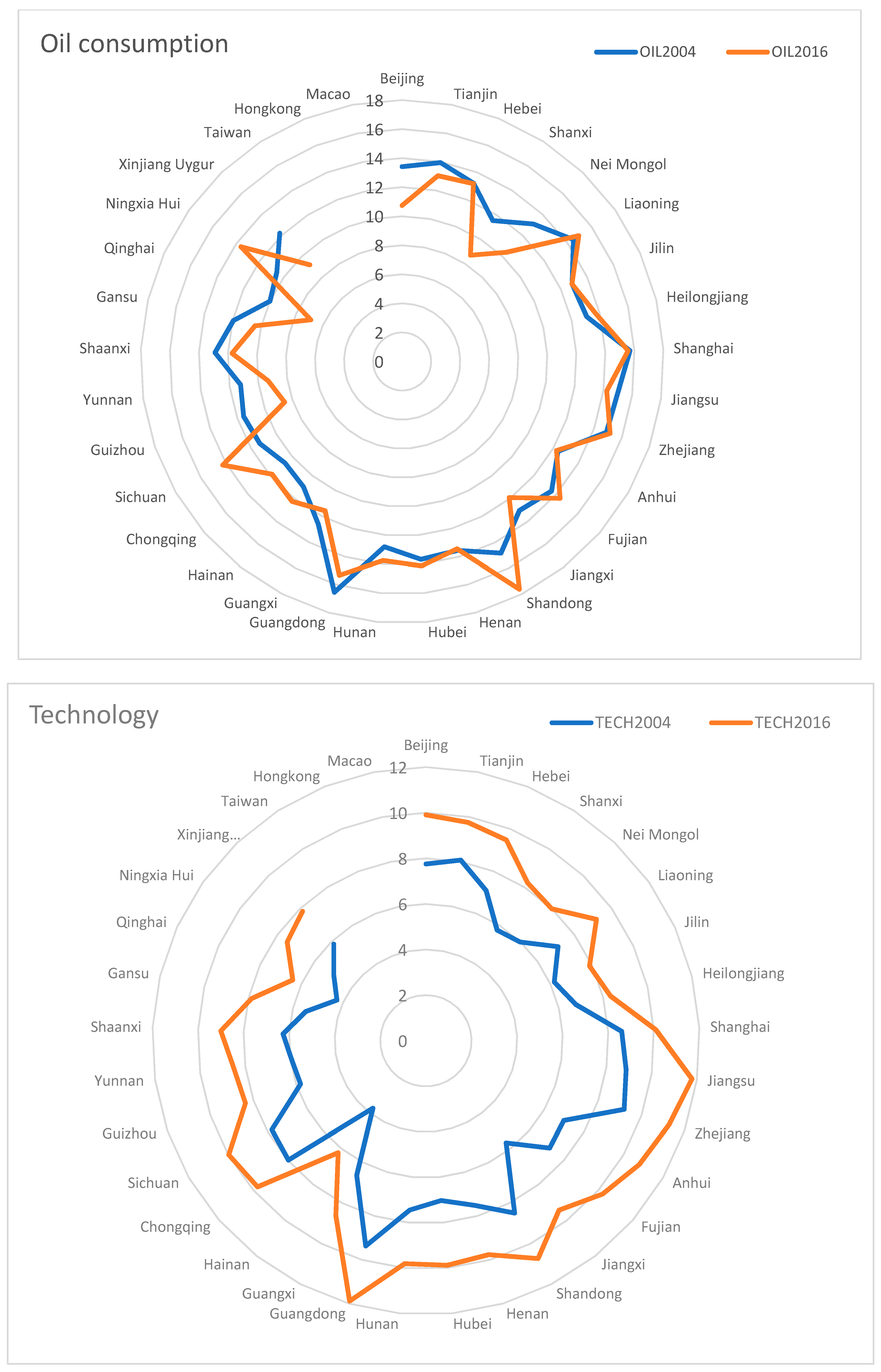
In this article, Area of Forested Land (AOF), Forest coverage rate (FCR), Forest Investment (FI) and Total Area of Afforestation (AFF) are considered as the main explanatory variables that are related to forestry. The data on the energy consumption and forest indicators are drawn from the National Bureau of Statistics of China (Data on energy sources and consumption are available at http://data.stats.gov.cn, accessed on 5 September 2019). In empirical estimations, we use per capita GDP, urbanization, and coal and oil consumption as control variables. The data on control variables are gathered from the China Statistical Yearbook. The GDP data are normalized to constant price (Chinese Yuan (CNY)).

Table 1. Variable definitions, unit of measurement and sources.

Variables	Definition	Unit of Measurement	Source
CO2	Energy-related CO2 emissions	Ton	IPCC (accessed on 5 September 2019)
URBAN	Percentage of the urban population in the total population	Percent	http://data.stats.gov.cn/english (accessed on 5 September 2019)
GDP	GDP divided by population at the end of the year	Yuan (CNY) in constant 1997 price	http://data.stats.gov.cn/english (accessed on 5 September 2019)
TECH	Number of patent applications of industrial enterprises above designated size	Piece	http://data.stats.gov.cn/english (accessed on 5 September 2019)
COAL	Consumption of coal	Ton	http://data.stats.gov.cn/english (accessed on 5 September 2019)
OIL	Consumption of Fuel Oil	Ton	http://data.stats.gov.cn/english (accessed on 5 September 2019)
AOF	Area of Forested Land	Hectare	http://data.stats.gov.cn/english (accessed on 5 September 2019)
FCR	Forest Coverage Rate	Percent	http://data.stats.gov.cn/english (accessed on 5 September 2019)
FI	Forest Investment	Yuan (CNY)	http://data.stats.gov.cn/english (accessed on 5 September 2019)
AFF	Total Area of Afforestation	Hectare	http://data.stats.gov.cn/english (accessed on 5 September 2019)

Note: All the variables are annual over 2004–2016.

reports the definition of variables, unit of measurement and data source of all variables used in the empirical models, while,

Table 2. Descriptive statistics.

Variable	Obs	Mean	Std. Dev.	Min	Max
CO2	390	3.3028	0.9736	1.4987	7.6977
URBAN	390	11.1604	1.6071	9.2341	16.0315
GDP	390	10.5659	1.0341	8.3658	14.7755
TECH	390	8.7944	1.4894	3.7612	11.8876
COAL	390	18.2850	0.9168	15.0162	19.8302
OIL	390	12.6624	2.1230	5.2983	17.6247
AOF	390	15.4900	1.4050	10.0213	17.6005
FCR	390	3.1772	0.7912	1.0647	4.1897
FI	390	15.0005	1.3312	10.4888	18.5033
AFF	390	4.5942	1.3737	−0.3425	6.7591

Note: All variables are in natural logarithms.

documents the descriptive statistics for our variables. In addition, the radar map in Figure 2 mentions that the studied variables have diversity across Chinese provinces.

Table 3. Correlation matrix.

	CO2	URBAN	GDP	TECH	COAL	OIL	AOF	FCR	FI	AFF
CO2	1.0000
URBAN	−0.1031 **	1.0000
	(0.0418)
GDP	0.8312 ***	−0.1829 ***	1.0000
	(0.0000)	(0.0003)
TECH	0.0327	−0.2777 ***	0.2788 ***	1.0000
	(0.5196)	(0.0000)	(0.0000)
COAL	0.2559 ***	−0.4436 ***	0.1771 ***	0.3040 ***	1.0000
	(0.0000)	(0.0000)	(0.0004)	(0.0000)
OIL	0.1075 **	−0.2829 ***	0.2633 ***	0.4306 ***	0.3157 ***	1.0000
	(0.0338)	(0.0000)	(0.0000)	(0.0000)	(0.0000)
AOF	−0.1555 ***	−0.0346	−0.2345 ***	−0.1827 ***	0.2974 ***	−0.2866 ***	1.0000
	(0.0021)	(0.4954)	(0.0000)	(0.0003)	(0.0000)	(0.0000)
FCR	−0.2690 ***	−0.1127 **	−0.0117	0.1439 ***	0.0767	0.2044 ***	0.4578 ***	1.0000
	(0.0000)	(0.0261)	(0.8176)	(0.0044)	(0.1304)	(0.0000)	(0.0000)
FI	0.0697	−0.2276 ***	0.2416 ***	0.1265 **	0.4215 ***	−0.0493	0.4273 ***	0.2266 ***	1.0000
	(0.1692)	(0.0000)	(0.0000)	(0.0124)	(0.0000)	(0.3315)	(0.0000)	(0.0000)
AFF	−0.0546	−0.0575	−0.1868 ***	−0.1902 ***	0.4548 ***	−0.3382 ***	0.7532 ***	0.1457 ***	0.5759 ***	1.0000
	(0.2824)	(0.2571)	(0.0002)	(0.0002)	(0.0000)	(0.0000)	(0.0000)	(0.0039)	(0.0000)

Notes: All variables are in natural logarithms; Numbers in the parentheses represent p-Values; ** denotes $p<0.05$; *** denotes $p<0.01$.

illustrates the correlation coefficients of all studied variables. The correlation findings indicate strong correlations between per capita CO₂ emissions and per capita GDP, while other correlation coefficients are relatively lower. To test for multi-collinearity problems, we use the variance inflation factor (VIF) test [58,59] for each predictor. The estimated VIF values of all all regression models are less than 10, which indicates the absence of multi-collinearity problems.

3.2. Model Specification

In this paper, we explore the factors that impact CO₂ emissions among Chinese provinces within both non-STIRPAT and STIRPAT model frameworks (Dietz and Rosa, 1997).

3.2.1. Non-STIRPAT Model

The non-STIRPAT model includes the forest variables, GDP, urbanization, coal and oil consumption, as given in Equation (2):

$$\begin{gathered} ln\left(C{O}_2{}_{i,t}\right)={\beta }_0+{\beta }_{1}ln\left(URBA{N}_{i,t}\right)+{\beta }_{2}ln\left(GD{P}_{i,t}\right)+{\beta }_{3}ln\left(COA{L}_{i,t}\right)+{\beta }_{4}ln\left(OI{L}_{i,t}\right)+{\beta }_{5}ln\left(FORES{T}_{i,t}\right)+{\mu }_i+u_{i,t}; \\ i=1,\dots ,N;t=1,\dots ,T \end{gathered}$$

(2)

where $FORES{T}_{i,t}=\left(AO{F}_{i,t},FC{R}_{i,t},F{I}_{i,t},AF{F}_{i,t}\right)$ denotes forestry variables for province $i$ at time $t$, and ${\mu }_i$ are assumed to be fixed province-specific effects. The observations in Equation (2) are available in the 30 contiguous provinces from 2004–2016, so that $T=13$ and $N=30$.

Based on the selected forest variables, Equation (2) can be divided into two broad specifications:

Models for forest coverage

Model 1.1:

$$\begin{gathered} ln\left(C{O}_2{}_{i,t}\right)={\beta }_0+{\beta }_{1}ln\left(URBA{N}_{i,t}\right)+{\beta }_{2}ln\left(GD{P}_{i,t}\right)+{\beta }_{3}ln\left(COA{L}_{i,t}\right) \\ +{\beta }_{4}ln\left(OI{L}_{i,t}\right)+{\beta }_{5}ln\left(AO{F}_{i,t}\right)+{\mu }_i+u_{i,t} \end{gathered}$$

Model 1.2:

$$\begin{gathered} ln\left(C{O}_2{}_{i,t}\right)={\beta }_0+{\beta }_{1}ln\left(URBA{N}_{i,t}\right)+{\beta }_{2}ln\left(GD{P}_{i,t}\right)+{\beta }_{3}ln\left(COA{L}_{i,t}\right) \\ +{\beta }_{4}ln\left(OI{L}_{i,t}\right)+{\beta }_{5}ln\left(FC{R}_{i,t}\right)+{\mu }_i+u_{i,t} \end{gathered}$$

Models for forest activities, investment and management

Model 2.1:

$$\begin{gathered} ln\left(C{O}_2{}_{i,t}\right)={\beta }_0+{\beta }_{1}ln\left(URBA{N}_{i,t}\right)+{\beta }_{2}ln\left(GD{P}_{i,t}\right)+{\beta }_{3}ln\left(COA{L}_{i,t}\right) \\ +{\beta }_{4}ln\left(OI{L}_{i,t}\right)+{\beta }_{5}ln\left(F{I}_{i,t}\right)+{\mu }_i+u_{i,t} \end{gathered}$$

Model 2.2:

$$\begin{gathered} ln\left(C{O}_2{}_{i,t}\right)={\beta }_0+{\beta }_{1}ln\left(URBA{N}_{i,t}\right)+{\beta }_{2}ln\left(GD{P}_{i,t}\right)+{\beta }_{3}ln\left(COA{L}_{i,t}\right) \\ +{\beta }_{4}ln\left(OI{L}_{i,t}\right)+{\beta }_{5}ln\left(AF{F}_{i,t}\right)+{\mu }_i+u_{i,t} \end{gathered}$$

In this paper, we expect that ${\beta }_2>0$ for GDP, ${\beta }_5>0$ for both AOF and FCR, and ${\beta }_5<0$ for both FI and AFF. The main reason behind positive ${\beta }_5$ coefficients is because proper forest management and forest investments can increase the forest role for the environment. However, the negative sign of ${\beta }_5$ coefficients may be due to the fact that forest management and afforestation activities might enhance the forest capabilities of carbon sink [3]. We also assume that ${\beta }_1<0$, ${\beta }_3>0$, and ${\beta }_4>0$.

3.2.2. Extended STIRPAT Model

After initial model estimations, we use an extended version of the STIRPAT model for robust analysis. The purpose of the extended STIRPAT model is to reaffirm the significance of forest activites to counter the environmental degradation process. The IPAT and STARPAT equation is as follows:

$$I=P\times A\times T$$

(3)

where $P$ is the population, which is proxied by urbanization (We have found the strong correlation between population and urbanization; however, we have to use one of these variables. We use urbanization, instead of population). $A$ is the affluence that is proxied by GDP, as followed by [60,61]. $T$ represents the technology, which is proxied by the number of patent applications from industrial enterprises above designated size and denoted by $TECH$.

$$I_{it}={\beta }_0{P}_{it}^{\beta }{A}_{it}^{\beta }{T}_{it}^{{\beta }_3}{\mu }_{it}$$

(4)

We use the natural log of Equation (4):

$$ln\left(I_{i,t}\right)={\beta }_0+{\beta }_{1}ln\left(P_{i,t}\right)+{\beta }_{2}ln\left(A_{i,t}\right)+{\beta }_{3}ln\left(T_{i,t}\right)+u_{i,t}$$

(5)

We transform Equation (5) by using the notations $I=C{O}_2,P=Urban,A=GDP,T=TECH$, as mentioned in Equation (6):

$$\begin{gathered} ln\left(C{O}_2{}_{i,t}\right)={\beta }_0+{\beta }_{1}ln\left(URBA{N}_{i,t}\right)+{\beta }_{2}ln\left(GD{P}_{i,t}\right)+{\beta }_{3}ln\left(TEC{H}_{i,t}\right) \\ +{\beta }_{4}ln\left(COA{L}_{i,t}\right)+{\beta }_{5}ln\left(OI{L}_{i,t}\right)+{\beta }_{6}ln\left(FORES{T}_{i,t}\right)+u_{i,t} \end{gathered}$$

(6)

where we shift the $FOREST$ variables by $AOF,FCR,FI$ and $AFF$.

STIRPAT models with forest coverage are as below:

Model 3.1:

$$\begin{gathered} ln\left(C{O}_2{}_{i,t}\right)={\beta }_0+{\beta }_{1}ln\left(URBA{N}_{i,t}\right)+{\beta }_{2}ln\left(GD{P}_{i,t}\right)+{\beta }_{3}ln\left(TEC{H}_{i,t}\right) \\ +{\beta }_{4}ln\left(COA{L}_{i,t}\right)+{\beta }_{5}ln\left(OI{L}_{i,t}\right)+{\beta }_{6}ln\left(AO{F}_{i,t}\right)+u_{i,t} \end{gathered}$$

(7)

Model 3.2:

$$\begin{gathered} ln\left(C{O}_2{}_{i,t}\right)={\beta }_0+{\beta }_{1}ln\left(URBA{N}_{i,t}\right)+{\beta }_{2}ln\left(GD{P}_{i,t}\right)+{\beta }_{3}ln\left(TEC{H}_{i,t}\right) \\ +{\beta }_{4}ln\left(COA{L}_{i,t}\right)+{\beta }_{5}ln\left(OI{L}_{i,t}\right)+{\beta }_{6}ln\left(FC{R}_{i,t}\right)+u_{i,t} \end{gathered}$$

(8)

STIRPAT models for forest activities, investment and management are as below:

Model 4.1:

$$\begin{gathered} ln\left(C{O}_2{}_{i,t}\right)={\beta }_0+{\beta }_{1}ln\left(URBA{N}_{i,t}\right)+{\beta }_{2}ln\left(GD{P}_{i,t}\right)+{\beta }_{3}ln\left(TEC{H}_{i,t}\right) \\ +{\beta }_{4}ln\left(COA{L}_{i,t}\right)+{\beta }_{5}ln\left(OI{L}_{i,t}\right)+{\beta }_{6}ln\left(F{I}_{i,t}\right)+u_{i,t} \end{gathered}$$

(9)

Model 4.2:

$$\begin{gathered} ln\left(C{O}_2{}_{i,t}\right)={\beta }_0+{\beta }_{1}ln\left(URBA{N}_{i,t}\right)+{\beta }_{2}ln\left(GD{P}_{i,t}\right)+{\beta }_{3}ln\left(TEC{H}_{i,t}\right)+ \\ {\beta }_{4}ln\left(COA{L}_{i,t}\right)+{\beta }_{5}ln\left(OI{L}_{i,t}\right)+{\beta }_{6}ln\left(AF{F}_{i,t}\right)+u_{i,t} \end{gathered}$$

(10)

The relationship between technology and carbon emissions is complex. Therefore, the impact of technological progress on the environment and the climate is still unclear.

4. Methodology

Spatial Dependence and Spatial Weight Matrix

The spatial dependence phenomenon indicates the interdependence of observations across different regions or provinces [62,63]. The global Moran’s I index [64] is employed to check the spatial features of the dependent variable, i.e., China’s provincial CO₂ emissions. Formally, this index is given by:

$$I=\frac{N}{{{\displaystyle \sum }}_{i=1}^n{{\displaystyle \sum }}_{j=1}^N{w}_{ij}}\frac{{{\displaystyle \sum }}_{i=1}^N{{\displaystyle \sum }}_{j=1}^N{w}_{ij}\left(y_i-\overline{y}\right)\left(y_j-\overline{y}\right)}{{{\displaystyle \sum }}_{i=1}^N{\left(y_i-\overline{y}\right)}^2};\forall i\ne j$$

(11)

where $\overline{y}$ denotes the sample average, $y_i$ shows the value of observed variables in the province $i$, $y_j$ represents the value of observed variables in another province $j$, and $w_{ij}$ stands for the spatial distance matrix with $w_{ii}=\forall i$ and $w_{ij}\ne 0\forall i\ne j$.

At a certain level of statistical significance, if $I>0$, this indicates positive global spatial autocorrelation. However, if $I<0$, this implies negative global spatial autocorrelation. Note that a random spatial distribution occurs if $I=0$. As argued by [65], a spatial clustering phenomenon exists if $I$ is significantly positive, while a significant negative $I$ indicates the evidence of a spatial dispersion across spatial units.

To test the statistical significance of the global spatial autocorrelation, a z-score and a p-Value are calculated. The $z_I$-score for the statistic $I$ is computed as follows:

$$z_I=\frac{I-E\left(I\right)}{\sqrt{V\left(I\right)}}⟶N\left(0,1\right)$$

(12)

where $E\left(I\right)=-1/\left(n-1\right)$ and $V\left(I\right)=E\left(I^2\right)-E^2\left(I\right)$.

The spatial autocorrelation is used to examine the local similarities and differences across neighboring provinces [66]. The local Moran’s I statistic is reported as:

$$I_i=\frac{z_i}{{{\displaystyle \sum }}_{i=1}^n{z}_i^2}\times z_i^{°}$$

(13)

where $z_i$ denotes the observation for province $i$ on per capita CO₂ emissions, and $z_i^{°}$ is the spatial lag for location $I$, obtained as follows:

$$z_i^{°}={{\displaystyle \sum }}_{j=1}^n{w}_{ij}{z}_j$$

(14)

The implementation of the local spatial autocorrelation allows the classification of each observation (i.e., province) into four classes or categories.

Table 4. VIF results.

VIF	Non-STIRPAT Specification				STIRPAT Specification
	Model 1.1	Model 1.2	Model 2.1	Model 2.2	Model 3.1	Model 3.2	Model 4.1	Model 4.2
URBAN	1.2914	1.2957	1.2968	1.3005	1.3042	1.3082	1.3097	1.3103
GDP	1.1588	1.1002	1.1606	1.1472	1.1794	1.1333	1.1884	1.1652
TECH	-	-	-	-	1.3548	1.3371	1.3324	1.3819
COAL	1.6187	1.3142	1.5721	2.2009	1.6703	1.3373	1.5897	2.3157
OIL	1.3862	1.2390	1.2892	1.6613	1.4847	1.3656	1.4345	1.7201
AOF	1.4144	-	-	-	1.4402	-	-	-
FCR	-	1.0535	-	-	-	1.0586	-	-
FI	-	-	1.3618	-	-	-	1.3636	-
AFF	-	-	-	1.9807	-	-	-	2.0571

Note: All variables are in natural logarithms.

reports the classifications as per Moran’s scatterplot. Using this figure, several spatial aspects of the distribution at different points can be visualized. Further, this scatterplot can be divided into four quadrants (I, II, III, and IV), as per the categories of regional disparities.

The average z-statistic of all provinces determines the spatial cluster types. For instance, if the z-statistic value is higher for any province than its average z-statistic, then the neighboring provinces’ scores might also be higher than the average, as reported in

Table 5. Local Moran classifications.

Quadrant	Spatial Cluster Type	Description	$\mathbf{Own}\mathbf{Value}{\mathit{z}}_{\mathit{i}}$	$\mathbf{Neighbor}’\mathbf{s}\mathbf{Value}{\mathit{z}}_{\mathit{i}}^{°}$
I	H–H	High values surrounded by high values.	Above average	Above average
II	L–H	Low values surrounded by high values.	Below average	Above average
III	L–L	Low values surrounded by low values.	Below average	Below average
IV	H–L	High values surrounded by low values.	Above average	Below average

. In such a scenario, these provinces can be categorized as High–High (H–H) cluster. In the same line, if the z-statistic value of any provinces is higher than the average score, but the neighboring province value is below average, that province is classified as High–Low (H–L) cluster. On the contrary, if the z-statistic of any province is observed as below average, but the neighbors’ scores are above average, that province is categorized as Low–High (L–H) cluster. Lastly, if both of the neighboring provinces have below-average z-statistics, these will fall into the Low–Low (L–L) cluster.

Spatial dependence is assumed to be closely related with the definition of the spatial weighting matrix $W$ [67]. Let ${\left\{X_i\right\}}_{i=1}^N$ denote the spatial data from $N$ provinces, and province $i$ is represented by the subscript $i$. In addition, $w_{ij}$ represents the distance between the province $i$ and the province $j$. In this article, we employ the binary weighting matrix technology, a widely used technique in energy-economics literature. Meanwhile, the study endorses the Rook adjacency rule, which states that two provinces having the same border can be considered as adjacent (The non-border provinces are classified as not adjacent). The spatial weighting matrix can be defined as:

$$w_{ij}=\{\begin{array}{l}1\mathrm{if}\mathrm{province}i\mathrm{and}\mathrm{province}jaregeographicallyadjacent,\\ 0\mathrm{otherwise}\end{array}$$

(15)

By convention, $w_{ii}=0\forall i$.

Table 6. Geographical adjacency information of 31 Chinese provinces.

Number	Province	Adjacent Province Number
1	Heilongjiang	2, 3
2	Nei Mongol (Neimenggu)	1, 3, 4, 7, 9, 10, 11, 14
3	Jilin	1, 2, 4
4	Liaoning	2, 3, 7
5	Xinjiang	9, 13, 18
6	Beijing	7, 8
7	Hebei	2, 4, 6, 8, 10, 12, 15
8	Tianjin	6, 7, 12
9	Gansu	2, 5, 11, 13, 14, 22
10	Shanxi	2, 7, 14, 15
11	Ningxia	2, 9, 14
12	Shandong	7, 8, 15, 16, 17
13	Qinghai	5, 9, 18, 22
14	Shaanxi	2, 9, 10, 11, 15, 20, 21, 22
15	Henan	7, 10, 12, 14, 17, 20
16	Jiangsu	12, 17, 19, 23
17	Anhui	12, 15, 16, 20, 23, 24
18	Tibet	5, 13, 22, 28
19	Shanghai	16, 23
20	Hubei	14, 15, 17, 21, 24, 25
21	Sichuan	14, 20, 22, 25, 26
22	Chongqing	9, 13, 14, 18, 21, 26, 28
23	Zhejiang	16, 17, 19, 24, 27
24	Jiangxi	17, 20, 23, 25, 27, 30
25	Hunan	20, 21, 24, 26, 29, 30
26	Guizhou	21, 22, 25, 28, 29
27	Fujian	23, 24, 30
28	Yunnan	18, 22, 26, 29
29	Guangxi	25, 26, 28, 30
30	Guangdong	24, 25, 27, 29, 30
31	Hainan	30

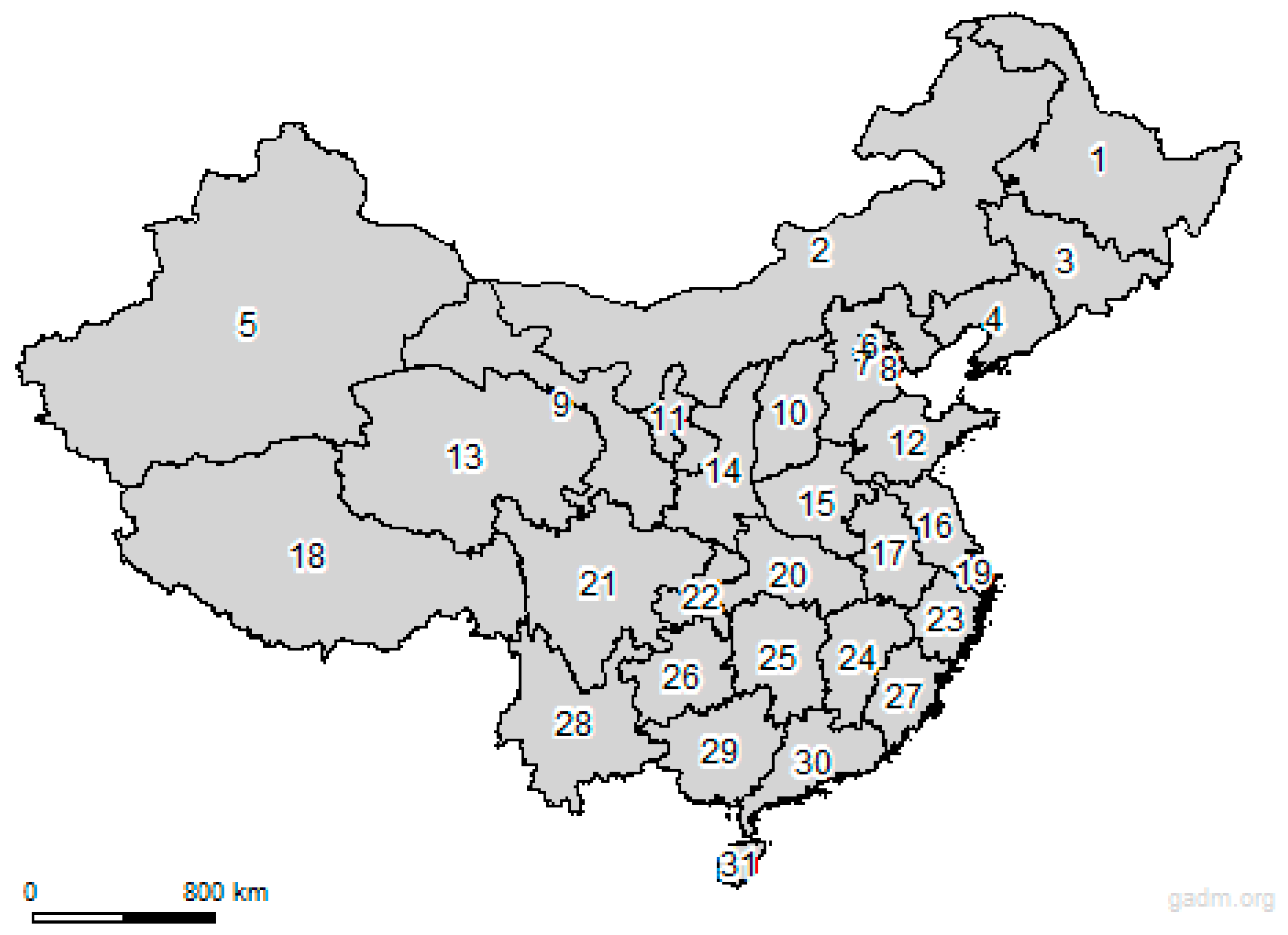
shows the spatial weighting matrix adjacent information for 31 Chinese provinces. According to the Rook adjacency rule, Hainan Province is not connected with other provinces since it is an island in China.

The unique identification code for each province is indicated by the number column. Moreover, the name of each province is represented by the province column. In addition, the province code adjacent to each province is indicated by the adjacent province code field. Furthermore, the spatial weighting matrix indicates that the distance between neighboring provinces is 1, while the distance between non-neighboring provinces is 0. Figure 3 illustrates a map of Chinese provinces and their corresponding numbers as per Table 6.

For the spatial econometrics model, estimation strategy and model interpretation, see Appendix A.

5. Empirical Results

5.1. Spatial Autocorrelation Analysis

We used the global Moran’s I index to test the existence of the spatial autocorrelation of the observations. Following [66], among others, a spatial clustering is captured with a significant positive Moran’s I value, while the significant negative values of Moran I indicate the spatial dispersion in Chinese provinces. Using data on all variables in 30 Chinese provinces, we calculated the global Moran’I index value for each year from 2004–2016, as well as the averaged values.

Table 7. Global Moran’s I of studied variables across Chinese provinces from 2004 to 2016.

Year	CO2	URBAN	GDP	TECH	COAL	OIL	AOF	FCR	FI	AFF
2004	0.3000 **	0.0789 *	−0.1290 **	0.2069 **	0.1488 **	0.3830 ***	0.2647 **	0.3532 ***	0.1566 **	0.3816 **
	(0.0110)	(0.0670)	(0.0480)	(0.0150)	(0.0110)	(0.0010)	(0.0400)	(0.0060)	(0.0300)	(0.0100)
2005	0.1740 **	0.0784 *	−0.1615 *	0.3100 **	0.1393 **	0.3720 ***	0.2646 **	0.3532 ***	0.1553 **	0.3367 **
	(0.0200)	(0.0670)	(0.0550)	(0.0100)	(0.0160)	(0.0010)	(0.0400)	(0.0060)	(0.0300)	(0.0200)
2006	0.1510 **	0.0774 *	0.0456	0.2090 **	0.1253 **	0.3830 ***	0.2646 **	0.3532 ***	0.1671 **	0.1363
	(0.0100)	(0.0670)	(0.1770)	(0.0300)	(0.0250)	(0.0010)	(0.0400)	(0.0060)	(0.0300)	(0.1000)
2007	0.1830 **	0.0762 *	0.0715 *	0.2970 **	0.1238 **	0.3080 ***	0.2646 **	0.3532 ***	0.1701 **	0.2070 *
	(0.0100)	(0.0690)	(0.0890)	(0.0290)	(0.0280)	(0.0030)	(0.0400)	(0.0060)	(0.0300)	(0.0700)
2008	0.1900 **	0.0751 *	−0.1390 **	0.2590 **	0.1097 **	0.3380 ***	0.2646 **	0.3532 ***	0.1651 **	0.2510 **
	(0.0100)	(0.0710)	(0.0490)	(0.0200)	(0.0380)	(0.0010)	(0.0200)	(0.0060)	(0.0300)	(0.0400)
2009	0.2050 **	0.0743 *	0.0974 **	0.3480 **	0.0977 *	0.3140 ***	0.2934 **	0.3391 ***	0.1598 **	0.2784 **
	(0.0100)	(0.0720)	(0.0490)	(0.0100)	(0.0560)	(0.0050)	(0.0200)	(0.0060)	(0.0300)	(0.0300)
2010	0.1070 *	0.0718 *	−0.1923 **	0.3010 **	0.1078 **	0.3080 ***	0.2934 **	0.3391 ***	0.1514 **	0.3801 **
	(0.0700)	(0.0790)	(0.0200)	(0.0340)	(0.0420)	(0.0010)	(0.0200)	(0.0060)	(0.0300)	(0.0100)
2011	0.1780 **	0.0715 *	−0.1994 **	0.3650 **	0.1032 **	0.4040 ***	0.2934 **	0.3391 ***	0.1032 **	0.2863 **
	(0.0100)	(0.0790)	(0.0120)	(0.0100)	(0.0480)	(0.0010)	(0.0200)	(0.0060)	(0.0300)	(0.0100)
2012	0.2300 **	0.0711 *	0.0940 *	0.3630 **	0.1021 *	0.3650 ***	0.2934 **	0.3391 ***	0.0921 **	0.2414 **
	(0.0100)	(0.0800)	(0.0750)	(0.0100)	(0.0510)	(0.0010)	(0.0200)	(0.0060)	(0.0400)	(0.0400)
2013	0.2260 **	0.0710 *	0.1053 **	0.3830 **	0.1080 **	0.3560 ***	0.2934 **	0.3391 ***	0.0872 **	0.2773 **
	(0.0100)	(0.0800)	(0.0370)	(0.0100)	(0.0460)	(0.0010)	(0.0200)	(0.0060)	(0.0400)	(0.0200)
2014	0.1350 **	0.0709 *	−0.1630 **	0.3910 **	0.1040 **	0.3500 ***	0.2934 **	0.3391 ***	0.0905 **	0.3046 **
	(0.0400)	(0.0800)	(0.0360)	(0.0100)	(0.0460)	(0.0010)	(0.0200)	(0.0060)	(0.0400)	(0.0100)
2015	0.1140 **	0.0712 *	−0.1970 **	0.3640 **	0.1003 *	0.3890 ***	0.2934 **	0.3391 ***	0.0908 *	0.3476 **
	(0.0400)	(0.0790)	(0.0430)	(0.0100)	(0.0550)	(0.0010)	(0.0200)	(0.0060)	(0.0400)	(0.0200)
2016	0.1540 **	0.0714 *	−0.0890 *	0.3780 **	0.0907 *	0.3970 ***	0.2934 **	0.3391 ***	0.0888 **	0.3604 **
	(0.0200)	(0.0790)	(0.0860)	(0.0100)	(0.0660)	(0.0010)	(0.0200)	(0.0060)	(0.0400)	(0.0200)
Average	0.2620 **	0.0739 *	0.1227 **	0.2070 **	0.1150 **	0.4390 ***	0.2635 **	0.03393 ***	0.1277 **	0.3959 **
	(0.0100)	(0.0730)	(0.0330)	(0.0300)	(0.0390)	(0.0010)	(0.0400)	(0.0050)	(0.0300)	(0.0100)

Notes: * denotes $p<0.1$; ** denotes $p<0.05$; *** denotes $p<0.01$; Numbers between parentheses represent pseudo p-Values.

summarizes the results of the global Moran’s I test for all variables. The $p$ Values are employed to check the statistical significance of the global Moran’s I values. As can be seen from Table 7, the global Moran’s I index is consistently positive and statistically significant at the 5% level. This finding indicates that air pollution in China exhibits significant positive spatial autocorrelation. The findings displayed in Table 7 also indicate that the global Moran’s I values are generally significant and positive for the remaining explanatory variables.

The global Moran’s I index reflects the overall distribution of spatial observations. The term “global” indicates that a single value for the index is generated for the whole pattern. Therefore, we cannot map the Global Moran’s I. Consequently, we use the Moran’s I scatter plot to visualize the spatial autocorrelation of variables. To save space, we only conduct a Moran’s I scatterplot of both environmental and forestry variables across Chinese provinces for the years 2004 and 2016 (see Figure 4). A visual inspection of Figure 4 confirms the previous results of the global Moran’s I and indicates the existence of spatial dependence for per capita CO₂ emission concentrations across Chinese provinces. Furthermore, the overall pattern of spatial dependence was also verified for forest variables.

For a better investigation of the spatial dependence pattern of both environmental and forestry variables across Chinese provinces, we used the local Moran’s I analysis, also known as the cluster and outlier analysis [64]. Global Moran’s I indices of spatial autocorrelation identify whether there is clustering in a variable’s values, but they do not indicate the location of clusters. To determine the location and magnitude of spatial autocorrelation, we should use local indices of spatial autocorrelation instead of global indices. Note that the term “local” implies that a value is produced for each spatial unit separately. Therefore, we can map the local Moran’s I indices (also known as local indicators of spatial association or LISA) as each spatial unit has a local Moran’s I value. Figure 5 depicts the LISA maps for environmental and forestry variables across Chinese provinces. Note that H–H and L–L clusters are the main types of agglomeration. Notably, the provinces having a high level of carbon are clustered with neighboring provinces that obtain the high values of per capita CO₂ emissions. In 2004, for example, the provinces with higher carbon level (H–H) were located in north China. The L–L group (e.g., low carbon emission provinces are clustered with neighboring provinces with similar values) are mainly concentrated in south China.

Furthermore, the distribution of Chinese provinces exhibits regional dynamic characteristics that vary across clusters. For instance, in 2004, the provinces in the H–H group and L–L groups were 9 and 9, respectively. The facts of 2004 show that the H–H and L–L groups were 54.55% of all Chinese provinces. On the contrary, we note that 45.45% of all provinces are in the other two groups (H–L and L–H). Such facts mainly imply that there was a dual structure in the spatial distribution of per capita CO₂ emissions in Chinese provinces in 2004. We further observe that in 2016, the number of H–H and L–L provinces had decreased by 4 and 9, respectively. The mentioned findings suggest that the spatial agglomeration of CO₂ emissions had decreased in the studied period from 2004 to 2016. From these results, we can draw the conclusion that the pattern of evolution of CO₂ emissions in Chinese provinces shows a certain path dependency effect.

We also employ the local Getis–Ord statistics of spatial autocorrelation [68] to identify statistically significant clusters of high values (hot spots) and clusters of low values (cold spots). These important statistics can reflect the extent of the clustering and dispersion of spatial objects. Knowing that the interference of the space is heterogeneous, the global correlation of spatial objects is also not certain in the distribution. It is therefore necessary to analyze the statistical significance in partial space based on local Getis–Ord statistics. Basically, we explore the hot spot analysis to identify if low or high values of per capita CO₂ emissions and forestry variables are spatially clustered, and create cold spots or hot spots, respectively. As shown in Figure 6, the reference values of per capita CO₂ emissions and forestry variables show territorial disparities. The findings include the high value clusters (hot spots), random (not significant), and the low value clusters (cold spots). In 2004, the high values (hot spots) of carbon emissions mainly clustered in north China. The low values (cold spots) mainly clustered in south China, while the random regions (not significant) were located in west China. The overall distribution of hot spots, cold spots, and randomness of the carbon emissions values in 2016 was not like that in 2004. The key difference was due to the expanded number of random regions. For forestry variables, we also observe some regional disparities, except for both AOF and FCR variables where we only found evidence of cold spots. Overall, the results indicate evidence of clustering for environmental and forestry variables across the Chinese provinces.

5.2. Cross-Sectional Dependence, Panel Unit Root and Panel Cointegration Tests

To correctly specify the empirical models described in the previous section, we start with a preliminary analysis of the study variables. We first test for the presence of non-stationarity in the variables, and therefore for the existence of a co-integration relationship in the different specifications. It is noteworthy that if all the variables are cointegrated, then the error term follows a stationary process. Therefore, regression analyses based on long-running relationships are not spurious, and it is possible to proceed with panel data models. Note that only 30 provinces (except Taiwan, Hong Kong, and Macao) are used in testing for cross-sectional dependence (CSD), panel unit root, and panel cointegration. The reason is that no data were available for those provinces. For coherence, we choose the data of 30 provinces for all variables.

The first step is to perform the CSD test for the variables to further examine whether spatial dependence across Chinese provinces exists [69]. Note that the CSD test does not require the specification of a spatial weighting matrix. The results are displayed in

Table 8. Pesaran’s CSD test for cross-sectional dependence.

Model	Model 1.1	Model 1.2	Model 2.1	Model 2.2	Model 3.1	Model 3.2	Model 4.1	Model 4.2
Pesaran’s CSD test	−1.9610 **	−2.1570 **	−2.0460 **	−1.9180 *	−2.3110 **	−2.4050 **	−2.5880 **	−2.3370 **
	(0.0498)	(0.0310)	(0.0408)	(0.0551)	(0.0190)	(0.0160)	(0.0112)	(0.0181)

Notes: Numbers in the parentheses represent p-Values; * denotes $p<0.1$; ** denotes $p<0.05$.

, where the null hypothesis that the variables are cross-sectionally independent is clearly rejected for all variables. This finding highlights the importance of considering the spatial dependence across Chinese provinces in this context. In the next step, we perform the panel unit root tests using the approaches of LLC [70], IPS [71], Breitung [72], H-T [73], Hadri [74], CIPS [75], and CADF [75]. The first five approaches refer to the first-generation unit root tests that ignore cross-sectional dependence. The last two approaches, i.e., the cross-sectionally augmented IPS (CIPS) and the cross-sectionally augmented Dickey–Fuller (CADF), are the second-generation unit root tests that assume the presence of cross-sectional dependence. Note that CIPS test is based on CADF regressions.

Due to the presence of cross-sectional dependence, we prefer using both CIPS and CADF tests since they produce consistent and reliable results.

Table 9. Panel unit root tests.

Variable		First Generation Panel Unit Root Tests					Second Generation Panel Unit Root Tests
		LLC	IPS	Breitung	H-T	Hadri	CIPS	CADF
CO2	Level	−4.0238 ***	−3.5401 ***	−7.0566 ***	0.0111 ***	6.0865 ***	−2.5090 ***	−1.2690
		(0.0000)	(0.0002)	(0.0000)	(0.0000)	(0.0000)		(0.9880)
	First Difference	−10.5922 ***	−12.3875 ***	−9.0587 ***	−0.5081 ***	5.3987 ***	−4.3240 ***	−2.0650 **
		(0.0000)	(0.0000)	(0.0000)	(0.0000)	(0.0000)		(0.0430)
URBAN	Level	−19.5027 ***	−9.2798 ***	−6.5217 ***	0.0959 ***	3.8801 ***	−2.9560 ***	−1.9640
		(0.0000)	(0.0000)	(0.0000)	(0.0000)	(0.0001)		(0.1120)
	First Difference	−12.9713 ***	−13.6673 ***	−8.3285 ***	−0.3551 ***	4.0725 ***	−4.8310 ***	−2.1160 **
		(0.0000)	(0.0000)	(0.0000)	(0.0000)	(0.0000)		(0.0240)
GDP	Level	1.3920	−1.2026	−7.9090 ***	−0.0008 ***	5.4276 ***	−2.6440 ***	−1.4530
		(0.9180)	(0.1146)	(0.0000)	(0.0000)	(0.0000)		(0.9080)
	First Difference	−17.2800 ***	−14.7527 ***	−9.4479 ***	−0.4705 ***	5.0312 ***	−4.2210 ***	−2.6530 ***
		(0.0000)	(0.0000)	(0.0000)	(0.0000)	(0.0000)		(0.0000)
TECH	Level	−3.0858 ***	−2.7315 ***	−6.0808 ***	0.3330 ***	4.7050 ***	−2.2060 **	−1.4960
		(0.0010)	(0.0032)	(0.0000)	(0.0000)	(0.0000)		(0.8680)
	First Difference	−9.6895 ***	−9.8381 ***	−8.9651 ***	−0.2210 ***	4.0515 ***	−3.3280 ***	−2.1440 **
		(0.0000)	(0.0000)	(0.0000)	(0.0000)	(0.0000)		(0.0170)
COAL	Level	−6.0586 ***	−4.3457 ***	−6.5162 ***	0.2989 ***	3.3762 ***	−2.2040	−1.6580
		(0.0000)	(0.0000)	(0.0000)	(0.0000)	(0.0004)		(0.6220)
	First Difference	−11.2558 ***	−8.8765 ***	−8.2800 ***	−0.1779 ***	3.3183 ***	−3.4390 ***	−2.1390 **
		(0.0000)	(0.0000)	(0.0000)	(0.0000)	(0.0005)		(0.0190)
OIL	Level	0.2999	−2.6042 ***	−6.8603 ***	0.0741 ***	5.5075 ***	−2.9920 ***	−1.5770
		(0.6179)	(0.0046)	(0.0000)	(0.0000)	(0.0000)		(0.7620)
	First Difference	−9.1241 ***	−12.4230 ***	−11.1131 ***	−0.5882 ***	5.4316 ***	−4.8210 ***	−2.3380 ***
		(0.0000	(0.0000	(0.0000)	(0.0000)	(0.0000)		(0.0010)
AOF	Level	−7.2087 ***	−4.7236 ***	−7.0323 ***	0.0961 ***	2.5494 ***	−2.6310 ***	−1.7780
		(0.0000)	(0.0000)	(0.0000)	(0.0000)	(0.0054)		(0.3870)
	First Difference	−14.4603 ***	−9.7230 ***	−8.3847 ***	−0.3963 ***	3.7074 ***	−4.0120 ***	−2.5100 ***
		(0.0000)	(0.0000)	(0.0000)	(0.0000)	(0.0001)		(0.0000)
FCR	Level	−4.3139 ***	−3.3473 ***	−5.9984 ***	0.2837 ***	4.8714 ***	−2.1130 *	−1.5870
		(0.0000)	(0.0004)	(0.0000)	(0.0000)	(0.0000)		(0.7460)
	First Difference	−12.6408 ***	−10.7530 ***	−8.0178 ***	−0.3836 ***	5.8667 ***	−3.6970 ***	−2.3540 ***
		(0.0000)	(0.0000)	(0.0000)	(0.0000)	(0.0000)		(0.0010)
FI	Level	−10.8826 ***	−6.2122 ***	−9.8212 ***	−0.2090 ***	3.6659 ***	−3.6160 ***	−1.9180
		(0.0000)	(0.0000)	(0.0000)	(0.0000)	(0.0001)		(0.1620)
	First Difference	−14.8183 ***	−15.6554 ***	−9.9365 ***	−0.6029 ***	3.4490 ***	−5.4370 ***	−3.0200 ***
		(0.0000)	(0.0000)	(0.0000)	(0.0000)	(0.0003)		(0.0000)
AFF	Level	−2.0748 **	−3.7332 ***	−6.6753 ***	0.1489 ***	2.0583 **	−2.5070 ***	−1.4040
		(0.0190)	(0.0000)	(0.0000)	(0.0000)	(0.0198)		(0.9420)
	First Difference	−7.7777 ***	−7.7801 ***	−8.0095	−0.4457 ***	3.2468 ***	−4.3780 ***	−4.3780 ***
		(0.0000)	(0.0000)	(0.0000)	(0.0000)	(0.0006)		(0.0000)

Notes: * denotes $p<0.1$; ** denotes $p<0.05$; *** denotes $p<0.01$. Numbers between parentheses represent p-Values.

reports the results of both the first- and second-generation unit root tests. As can be seen, all variables are integrated of order 1, i.e., I(1). Accordingly, it is mandatory to go for the third step by testing for panel cointegration, which allows for long-running relationships between variables. To do so, we firstly use the residual-based panel cointegration tests, in particular those suggested by [76,77]. Then, we perform the error-correction-based panel cointegration tests [78]. Note that the Westerlund cointegration methodologies have an advantage over the others, in terms of allowing for cross-sectional dependence.

Table 10. Panel cointegration tests.

Model	Model 1.1	Model 1.2	Model 2.1	Model 2.2	Model 3.1	Model 3.2	Model 4.1	Model 4.2
Pedroni (1990, 2004) Cointegration Tests
$H_0$: no cointegration versus $H_1$: common AR coefficients (within-dimension)
Modified variance ratio	−6.5533 ***	−6.1835 ***	−6.1617 ***	−6.2143 ***	−7.4406 ***	−7.1901 ***	−7.1219 ***	−7.2279 ***
	(0.0000)	(0.0000)	(0.0000)	(0.0000)	(0.0000)	(0.0000)	(0.0000)	(0.0000)
Modified Phillips–Perron t	4.1802 ***	3.7005 ***	4.1246 ***	3.5493 ***	5.7154 ***	5.0610 ***	5.1688 ***	4.8714 ***
	(0.0000)	(0.0001)	(0.0000)	(0.0002)	(0.0000)	(0.0000)	(0.0000)	(0.0000)
Phillips–Perron t	−3.5330 ***	−4.7858 ***	−3.1533 ***	−5.4806 ***	−4.6003 ***	−6.5528 ***	−4.0233 ***	−6.7724 ***
	(0.0002)	(0.0000)	(0.0008)	(0.0000)	(0.0000)	(0.0000)	(0.0000)	(0.0000)
Augmented Dickey–Fuller t	−3.3015 ***	−5.0023 ***	−3.0742 ***	−5.1378 ***	−4.5530 ***	−7.4256 ***	−4.2540 ***	−6.6357 ***
	(0.0005)	(0.0000)	(0.0011)	(0.0000)	(0.0000)	(0.0000)	(0.0000)	(0.0000)
$H_0$: no cointegration versus $H_1$: individual AR coefficients (between-dimension)
Modified Phillips–Perron t	6.5593 ***	6.3329 ***	6.7115 ***	6.1656 ***	8.1066 ***	7.3256 ***	7.6147 ***	7.3000 ***
	(0.0000)	(0.0000)	(0.0000)	(0.0000)	(0.0000)	(0.0000)	(0.0000)	(0.0000)
Phillips–Perron t	−3.4486 ***	−3.2880 ***	−2.0605 **	−4.9606 ***	−7.0493 ***	−7.7295 ***	−4.4056 ***	−7.9471 ***
	(0.0003)	(0.0005)	(0.0197)	(0.0000)	(0.0000)	(0.0000)	(0.0000)	(0.0000)
Augmented Dickey–Fuller t	−3.0782 ***	−3.7863 ***	−1.7462 **	−4.8109 ***	−4.7442 ***	−8.8345 ***	−4.2545 ***	−7.3720 ***
	(0.0010)	(0.0001)	(0.0404)	(0.0000)	(0.0000)	(0.0000)	(0.0000)	(0.0000)
Westerlund (2007) error correction panel cointegration tests
$H_0$: no cointegration versus $H_1$: some panels are cointegrated
Variance ratio	7.5618 ***	5.6804 ***	7.0989 ***	7.1416 ***	9.1870 ***	9.3259 ***	9.1271 ***	9.0588 ***
	(0.0000)	(0.0000)	(0.0000)	(0.0000)	(0.0000	(0.0000)	(0.0000	(0.0000
$H_0$: no cointegration versus $H_1$: all panels are cointegrated
Variance ratio	1.8140 **	0.7598	1.6135 *	2.1466 **	2.1882 **	2.2052 **	2.3034 **	2.4576 ***
	(0.0348)	(0.2237)	(0.0533)	(0.0159)	(0.0143	(0.0137)	(0.0106	(0.0070

Notes: * denotes $p<0.1$; ** denotes $p<0.05$; *** denotes $p<0.01$. Numbers between parentheses represent p-Values.

reports the results of both Pedroni [76,77] and Westerlund [78] panel-data cointegration tests. All test statistics reject the null hypothesis of no cointegration in favor of the alternative hypothesis of cointegration between the variables. Therefore, we explore the long-run relationship in the next subsection.

5.3. Econometric Results

To analyze the model’s accuracy on selected data, we first conduct a non-spatial panel model approach. Afterwards, we examine the existence of a spatial correlation between spatial units by using classical LM tests. In rejecting the non-spatial panel model, we choose the best fit spatial panel model for empirical estimations. The empirical estimations of non-spatial panel models are displayed in

Table 11. Estimation results without spatial interaction effects under non-STIRPAT specification.

$\mathbf{Dependent}\mathbf{Variable}:\mathbf{C}{\mathbf{O}}_2$	Model 1.1		Model 1.2		Model 2.1		Model 2.2
	Pooled OLS	Spatial Fixed Effects	Pooled OLS	Spatial Fixed Effects	Pooled OLS	Spatial Fixed Effects	Pooled OLS	Spatial Fixed Effects
URBAN	0.0600 ***	−2.7225 ***	0.0482 ***	−2.0774 ***	0.0471 ***	−1.2072 ***	0.0613 ***	−2.5298 ***
	(0.0009)	(0.0000)	(0.0030)	(0.0000)	(0.0036)	(0.0000)	(0.0008)	(0.0000)
GDP	0.7891 ***	0.9216 ***	0.7864 ***	0.9356 ***	0.8624 ***	0.9492 ***	0.7953 ***	0.9236 ***
	(0.0000)	(0.0000)	(0.0000)	(0.0000)	(0.0000)	(0.0000)	(0.0000)	(0.0000)
COAL	0.2448 ***	−0.3309 ***	0.2059 ***	−0.2504 ***	0.3362 ***	−0.0280	0.2492 ***	−0.2749 ***
	(0.0000)	(0.0000)	(0.0000)	(0.0000)	(0.0000)	(0.5099)	(0.0000)	(0.0000)
OIL	−0.0824 ***	0.0375 ***	−0.0464 ***	0.0367 ***	−0.1033 ***	0.0423 ***	−0.0826 ***	0.0300 **
	(0.0000)	(0.0033)	(0.0001)	(0.0027)	(0.0000)	(0.0000)	(0.0000)	(0.0123)
AOF	−0.0524 **	−0.0371	-	-	-	-	-	-
	(0.0154)	(0.6792)	-	-	-	-	-	-
FCR	-	-	−0.3008 ***	−0.4272 ***	-	-	-	-
	-	-	(0.0000)	(0.0000)	-	-	-	-
FI	-	-	-	-	−0.2036 ***	−0.1864 ***	-	-
	-	-	-	-	(0.0000)	(0.0000)	-	-
AFF	-	-	-	-	-	-	−0.0415	−0.1368 ***
	-	-	-	-	-	-	(0.1135)	(0.0000)
Intercept	−8.3261 ***	-	−7.7654 ***	-	−8.1202 ***	-	−9.1033 ***	-
	(0.0000)	-	(0.0000)	-	(0.0000)	-	(0.0000)	-
$R^2$	0.7379	0.9310	0.7905	0.9365	0.7907	0.9552	0.7355	0.9395
${\overline{R}}^2$	0.7344	0.9303	0.7878	0.9358	0.7880	0.9547	0.7321	0.9389
${\sigma }^2$	0.2517	0.0475	0.2011	0.0438	0.2010	0.0309	0.2540	0.0417
FE $R^2$	-	0.9504	-	0.9543	-	0.9678	-	0.9565
Log-Likelihood	−281.3911	43.1883	−237.6363	59.1674	−237.4793	127.3324	−283.1005	68.8650
AIC
BIC
$L{R}_{SFE}$ test	-	649.1588 ***	-	593.6073 ***	-	729.6234 ***	-	703.9312 ***
	-	(0.0000)	-	(0.0000)	-	(0.0000)	-	(0.0000)
LM spatial lag	6.0425 ***	4.9957 **	8.7386 ***	6.2079 **	6.9798 ***	3.2168 *	6.3872 ***	5.4466 **
	(0.0015)	(0.0250)	(0.0039)	(0.0130)	(0.0080)	(0.0730)	(0.0012)	(0.0200)
Robust LM spatial lag	40.2026 ***	30.5051 ***	26.8402 ***	22.6795 ***	4.5700 **	18.3031 ***	34.2431 ***	22.7681 ***
	(0.0000)	(0.0000)	(0.0000)	(0.0000)	(0.0330)	(0.0000)	(0.0000)	(0.0000)
LM spatial error	147.4629 ***	139.8998 ***	107.5845 ***	150.4542 ***	76.1024 ***	79.2805 ***	137.2371 ***	108.2111 ***
	(0.0000)	(0.0000)	(0.0000)	(0.0000)	(0.0000)	(0.0000)	(0.0000)	(0.0000)
Robust LM spatial error	185.6230 ***	168.7544 ***	133.6860 ***	172.7489 ***	73.6925 ***	79.2805 ***	169.0931 ***	129.1053 ***
	(0.0000)	(0.0000)	(0.0000)	(0.0000)	(0.0000)	(0.0000)	(0.0000)	(0.0000)

Notes: All variables are in natural logarithms; Numbers in the parentheses represent p-Values; * denotes $p<0.1$; ** denotes $p<0.05$; *** denotes $p<0.01$. LM tests compare the classic pooled OLS regression against the alternative spatial autoregressive and spatial error model specifications under the null of no spatial dependence. LM spatial lag + robust LM spatial error = LM spatial error + robust LM spatial lag. The likelihood ratio for fixed effects $\left(L{R}_{SFE}\right)$ tests for the existence of a spatial fixed effect against the Pooled OLS specification.

and

Table 12. Estimation results without spatial interaction effects under STIRPAT specification.

$\mathbf{Dependent}\mathbf{Variable}:\mathbf{C}{\mathbf{O}}_2$	Model 3.1		Model 3.2		Model 4.1		Model 4.2
	Pooled OLS	Spatial Fixed Effects	Pooled OLS	Spatial Fixed Effects	Pooled OLS	Spatial Fixed Effects	Pooled OLS	Spatial Fixed Effects
URBAN	0.0456 ***	−2.6251 ***	0.0358 **	−2.0058 ***	0.0340 **	−1.2082 ***	0.0486 ***	−2.4288 ***
	(0.0060)	(0.0000)	(0.0164)	(0.0000)	(0.0216)	(0.0000)	(0.0036)	(0.0000)
GDP	0.8173 ***	0.9260 ***	0.8178 ***	0.9395 ***	0.8923 ***	0.9501 ***	0.8219 ***	0.9285 ***
	(0.0000)	(0.0000)	(0.0000)	(0.0000)	(0.0000)	(0.0000)	(0.0000)	(0.0000)
TECH	−0.1594 ***	−0.0332 ***	−0.1383 ***	−0.0322 ***	−0.1437 ***	−0.0112	−0.1622 ***	−0.0386 ***
	(0.0000)	(0.0011)	(0.0000)	(0.0009)	(0.0000)	(0.1794)	(0.0000)	(0.0000)
COAL	0.2953 ***	−0.3316 ***	0.2354 ***	−0.2542 ***	0.3630 ***	−0.0346	0.3251 ***	−0.2762 ***
	(0.0000)	(0.0000)	(0.0000)	(0.0000)	(0.0000)	(0.4182)	(0.0000)	(0.0000)
OIL	−0.0522 ***	0.0343 ***	−0.0165	0.0336 ***	−0.0700 ***	0.0411 ***	−0.0592 ***	0.0259 **
	(0.0001)	(0.0067)	(0.1511)	(0.0056)	(0.0000)	(0.0001)	(0.0001)	(0.0276)
AOF	−0.0757 ***	−0.0536	-	-	-	-	-	-
	(0.0002)	(0.5458)	-	-	-	-	-	-
FCR	-	-	−0.2847 ***	−0.4246 ***	-	-	-	-
	-	-	(0.0000)	(0.0000)	-	-	-	-
FI	-	-	-	-	−0.1976 ***	−0.1831 ***	-	-
	-	-	-	-	(0.0000)	(0.0000)	-	-
AFF	-	-	-	-	-	-	−0.0829 ***	−0.1426 ***
	-	-	-	-	-	-	(0.0007)	(0.0000)
Intercept	−8.0067 ***	-	−7.7115 ***	-	−8.0274 ***	-	−9.3135 ***	-
	(0.0000)	-	(0.0000)	-	(0.0000)	-	(0.0000)	-
$R^2$	0.7817	0.9329	0.8240	0.9382	0.8270	0.9554	0.7801	0.9421
${\overline{R}}^2$	0.7783	0.9321	0.8213	0.9374	0.8243	0.9548	0.7767	0.9413
${\sigma }^2$	0.2101	0.0463	0.1694	0.0427	0.1666	0.0308	0.2117	0.0400
FE $R^2$	-	0.9517	-	0.9556	-	0.9679	-	0.9583
Log-likelihood	−245.6664	48.6134	−203.6707	64.7395	−200.3567	128.2492	−247.1257	77.2708
AIC	505.3328	−85.2268	421.3414	−117.4790	414.7134	−244.4984	508.2514	−142.5416
BIC	533.0958	−61.4299	449.1044	−93.6821	442.4764	−220.7015	536.0144	−118.7447
$L{R}_{SFE}$ test	-	588.5595 ***	-	536.8205 ***	-	657.2117 ***	-	648.7929 ***
	-	(0.0000)	-	(0.0000)	-	(0.0000)	-	(0.0000)
LM spatial lag	1.9706	0.6663	0.9624	0.0275	8.1901 ***	2.6166	2.2546	0.6986
	(0.1600)	(0.4140)	(0.3270)	(0.8680)	(0.0040)	(0.1060)	(0.1330)	(0.4030)
Robust LM spatial lag	36.0600 ***	26.5160 ***	22.0992 ***	18.9143 ***	3.1963 *	17.4096 ***	27.7516 ***	16.7469 ***
	(0.0000)	(0.0000)	(0.0000)	(0.0000)	(0.0740)	(0.0000)	(0.0000)	(0.0000)
LM spatial error	166.5619 ***	149.6885 ***	119.1124 ***	156.7407 ***	90.4599 ***	83.4037 ***	143.0127 ***	102.3248 ***
	(0.0000)	(0.0000)	(0.0000)	(0.0000)	(0.0000)	(0.0000)	(0.0000)	(0.0000)
Robust LM spatial error	200.6513 ***	175.5382 ***	140.2493 ***	175.6275 ***	85.4662 ***	98.1967 ***	168.5096 ***	118.3731 ***
	(0.0000)	(0.0000)	(0.0000)	(0.0000)	(0.0000)	(0.0000)	(0.0000)	(0.0000)

Notes: All variables are in natural logarithms; Numbers in the parentheses represent p-Values; * denotes $p<0.1$; ** denotes $p<0.05$; *** denotes $p<0.01$. LM tests compare the classic pooled OLS regression against the alternative spatial autoregressive and spatial error model specifications under the null of no spatial dependence. LM spatial lag + robust LM spatial error = LM spatial error + robust LM spatial lag. The likelihood ratio for fixed effects $\left(L{R}_{SFE}\right)$ tests for the existence of a spatial fixed effect against the Pooled OLS specification.

. The empirics in these Tables report the likelihood ratio (LR) test, which allows us to decide between the spatial fixed effects and the pooled OLS techniques. The empirical results indicate that the spatial fixed effects method can report the most reliable and robust findings. In diagnostic testing, we use the classical LM and robust LM tests [67,79] to check the spatial dependence in models. The diagnostic findings show that the hypotheses can be rejected if: (a) there is no geographically lagged dependent variable; and (b) there are no spatially autocorrelated error term in the models. The findings are in line with the conclusions of [80]. The empirical results suggest that there might be a spatial correlation in the studied variables. Hence, in such a condition, the spatial panel data models can be more favorable for consistent, robust, and valid outcomes than non-spatial interaction effects.

To examine the appropriate technique for the spatial panel model, we use the panel spatial Durbin model (SDM) and then apply the Wald and LR tests [81]. The findings of the panel SDM are given in Table 8. Referring to the empirics of Wald and LR tests, we report the rejection of null hypotheses. The empirical outcomes of

Table 13. Estimation results with spatial interaction effects under non-STIRPAT specification.

$\mathbf{Dependent}\mathbf{Variable}:\mathbf{C}{\mathbf{O}}_2$	Model 1.1		Model 1.2		Model 2.1		Model 2.2
	SAR-FE	SDM-FE	SAR-FE	SDM-FE	SAR-FE	SDM-FE	SAR-FE	SDM-FE
$W\ast {\mathrm{CO}}_2\left(\delta \right)$	−0.0320	0.8090 ***	−0.0150	0.8200 ***	−0.0360 *	0.6970 ***	−0.0310	0.7720 ***
	(0.1898)	(0.0000)	(0.5201)	(0.0000)	(0.0617)	(0.0000)	(0.1672)	(0.0000)
$URBAN$	−2.6802 ***	−0.8801 ***	−2.0582 ***	−0.7293 ***	−1.1332 ***	−0.7202 ***	−2.4683 ***	−0.7921 ***
	(0.0000)	(0.0000)	(0.0000)	(0.0000)	(0.0000)	(0.0000)	(0.0000)	(0.0000)
$GDP$	0.9231 ***	0.9790 ***	0.9361 ***	0.9796 ***	0.9511 ***	0.9795 ***	0.9252 ***	0.9779 ***
	(0.0000)	(0.0000)	(0.0000)	(0.0000)	(0.0000)	(0.0000)	(0.0000)	(0.0000)
$COAL$	−0.3195 ***	0.3774 ***	−0.2450 ***	0.3953 ***	−0.0113	0.4078 ***	−0.2610 ***	0.3869 ***
	(0.0000)	(0.0000)	(0.0000)	(0.0000)	(0.8005)	(0.0000)	(0.0000)	(0.0000)
$OIL$	0.0366 ***	0.0297 ***	0.0363 ***	0.0298 ***	0.0412 ***	0.0308 ***	0.0291 **	0.0295 ***
	(0.0052)	(0.0000)	(0.0040)	(0.0000)	(0.0001)	(0.0000)	(0.0180)	(0.0000)
$AOF$	−0.0186	0.1748 ***	-	-	-	-	-	-
	(0.8427)	(0.0009)	-	-	-	-	-	-
$FCR$	-	-	−0.4206 ***	0.0817 *	-	-	-	-
	-	-	(0.0000)	(0.0884)	-	-	-	-
$FI$	-	-	-	-	−0.1867 ***	−0.0220 **	-	-
	-	-	-	-	(0.0000)	(0.0385)	-	-
$AFF$	-	-	-	-	-	-	−0.1366 ***	−0.0410 ***
	-	-	-	-	-	-	(0.0000)	(0.0000)
$W\ast URBAN$	-	1.0077 ***	-	0.9617 ***	-	1.6786 ***	-	0.9661 ***
	-	(0.0006)	-	(0.0008)	-	(0.0000)	-	(0.0019)
$W\ast GDP$	-	−0.7964 ***	-	−0.8011 ***	-	−0.6841 ***	-	−0.7589 ***
	-	(0.0000)	-	(0.0000)	-	(0.0000)	-	(0.0000)
$W\ast COAL$	-	−0.5076 ***	-	−0.4728 ***	-	−0.4440 ***	-	−0.5179 ***
	-	(0.0000)	-	(0.0000)	-	(0.0000)	-	(0.0000)
$W\ast OIL$	-	−0.0536 ***	-	−0.0530 ***	-	−0.0437 ***	-	−0.0456 ***
	-	(0.0001)	-	(0.0001)	-	(0.0013)	-	(0.0008)
$W\ast AOF$	-	−0.2930 ***	-	-	-	-	-	-
	-	(0.0066)	-	-	-	-	-	-
$W\ast FCR$	-	-	-	−0.2628 ***	-	-	-	-
	-	-	-	(0.0007)	-	-	-	-
$W\ast FI$	-	-	-	-	-	−0.0718 ***	-	-
	-	-	-	-	-	(0.0000)	-	-
$W\ast AFF$	-	-	-	-	-		-	−0.0255 *
	-	-	-	-	-		-	(0.0915)
$R^2$	0.9506	0.9897	0.9543	0.9898	-	0.9899	0.9567	0.9898
Corrected $R^2$	0.9332	0.9596	0.9374	0.9554	-	0.9740	0.9413	0.9657
${\sigma }^2$	0.0506	0.0098	0.0468	0.0097	0.0327	0.0096	0.0443	0.0097
Log-likelihood	43.4339	305.8576	58.7586	306.1607	128.4496	324.0281	69.2451	312.8724
Hausman test	119.3149 ***	404.9065 ***	70.0293 ***	414.2877 ***	27.2294 ***	273.9556 ***	103.5680 ***	477.2330 ***
	(0.0000)	(0.0000)	(0.0000)	(0.0000)	(0.0001)	(0.0000)	(0.0000)	(0.0000)
Wald test spatial lag	-	1412.8000 ***	-	1394.7000 ***	-	813.5494 ***	-	1162.3000 ***
	-	(0.0000)	-	(0.0000)	-	(0.0000)	-	(0.0000)
LR test spatial lag	-	523.6306 ***	-	493.5876 ***	-	389.9405 ***	-	486.0380 ***
	-	(0.0000)	-	(0.0000)	-	(0.0000)	-	(0.0000)
Wald test spatial error	-	45.2534 ***	-	42.0532 ***	-	75.0870 ***	-	53.2683 ***
	-	(0.0000)	-	(0.0000)	-	(0.0000)	-	(0.0000)
LR test spatial error	-	40.6568 ***	-	45.5991 ***	-	80.6870 ***	-	47.8657 ***
	-	(0.0000)	-	(0.0000)	-	(0.0000)	-	(0.0000)

Notes: All variables are in natural logarithms; Numbers in the parentheses represent p-Values; * denotes $p<0.1$; ** denote $p<0.05$; *** denotes $p<0.01$.

and

Table 14. Estimation results with spatial interaction effects under STIRPAT specification.

$\mathbf{Dependent}\mathbf{Variable}:\mathbf{C}{\mathbf{O}}_2$	Model 3.1		Model 3.2		Model 4.1		Model 4.2
	SAR-FE	SDM-FE	SAR-FE	SDM-FE	SAR-FE	SDM-FE	SAR-FE	SDM-FE
$W\ast {\mathrm{CO}}_2\left(\delta \right)$	−0.0200	0.8220 ***	−0.0040	0.8200 ***	−0.0330 *	0.6990 ***	−0.0190	0.7730 ***
	(0.3937)	(0.0000)	(0.8633)	(0.0000)	(0.0888)	(0.0000)	(0.3934)	(0.0000)
URBAN	−2.6025 ***	−0.8776 ***	−2.0012 ***	−0.7300 ***	−1.1402 ***	−0.7121 ***	−2.3942 ***	−0.8342 ***
	(0.0000)	(0.0000)	(0.0000)	(0.0000)	(0.0000)	(0.0000)	(0.0000)	(0.0000)
GDP	0.9267 ***	0.9794 ***	0.9396 ***	0.9799 ***	0.9517 ***	0.9789 ***	0.9294 ***	0.9790 ***
	(0.0000)	(0.0000)	(0.0000)	(0.0000)	(0.0000)	(0.0000)	(0.0000)	(0.0000)
TECH	−0.0319 ***	−0.0106 *	−0.0320 ***	−0.0124 **	−0.0091	−0.0099 *	−0.0374 ***	−0.0141 **
	(0.0016)	(0.0753)	(0.0015)	(0.0370)	(0.2913)	(0.0953)	(0.0001)	(0.0183)
COAL	−0.3245 ***	0.3688 ***	−0.2528 ***	0.3838 ***	−0.0181	0.3984 ***	−0.2676 ***	0.3802 ***
	(0.0000)	(0.0000)	(0.0000)	(0.0000)	(0.6893)	(0.0000)	(0.0000)	(0.0000)
OIL	0.0338 ***	0.0289 ***	0.0335 ***	0.0288 ***	0.0404 ***	0.0303 ***	0.0255 **	0.0286 ***
	(0.0067)	(0.0000)	(0.0071)	(0.0000)	(0.0001)	(0.0000)	(0.0351)	(0.0000)
AOF	−0.0414	0.1666 ***	-	-	-	-	-	-
	(0.6417)	(0.0015)	-	-	-	-	-	-
FCR	-		−0.4228 ***	0.0810 *	-	-	-	-
	-		(0.0000)	(0.0894)	-	-	-	-
FI	-		-		−0.1840 ***	−0.0195 *	-	-
	-		-		(0.0000)	(0.0672)	-	-
AFF	-		-		-	-	−0.1424 ***	−0.0419 ***
	-		-		-	-	(0.0000)	(0.0000)
$W\ast URBAN$	-	1.0410 ***	-	0.9562 ***	-	1.6258 ***	-	1.1258 ***
	-	(0.0004)	-	(0.0010)	-	(0.0000)	-	(0.0004)
$W\ast GDP$	-	−0.8056 ***	-	−0.7980 ***	-	−0.6850 ***	-	−0.7553 ***
	-	(0.0000)	-	(0.0000)	-	(0.0000)	-	(0.0000)
$W\ast TECH$	-	0.0044	-	0.0047	-	0.0124	-	−0.0022
	-	(0.5674)	-	(0.5436)	-	(0.1079)	-	(0.7773)
$W\ast COAL$	-	−0.4927 ***	-	−0.4610 ***	-	−0.4331 ***	-	−0.5084 ***
	-	(0.0000)	-	(0.0000)	-	(0.0000)	-	(0.0000)
$W\ast OIL$	-	−0.0543 ***	-	−0.0540 ***	-	−0.0403 ***	-	−0.0500 ***
	-	(0.0001)	-	(0.0001)	-	(0.0036)	-	(0.0002)
$W\ast AOF$	-	−0.2881 ***	-	-	-	-	-	-
	-	(0.0076)	-	-	-	-	-	-
$W\ast FCR$	-	-	-	−0.2685 ***	-	-	-	-
	-	-	-	(0.0005)	-	-	-	-
$W\ast FI$	-	-	-	-	-	−0.0744 ***	-	-
	-	-	-	-	-	(0.0000)	-	-
$W\ast AFF$	-	-	-	-	-	-	-	−0.0380 **
	-	-	-	-	-	-	-	(0.0152)
$R^2$	0.9518	0.9899	0.9556	0.9899	0.9682	0.9900	0.9584	0.9900
Corrected $R^2$	0.9342	0.9583	0.9385	0.9559	0.9567	0.9743	0.9430	0.9677
${\sigma }^2$	0.0455	0.0096	0.0455	0.0095	0.0326	0.0095	0.0426	0.0094
Log-likelihood	48.9595	307.6443	64.1455	308.6774	129.0525	325.6929	77.0280	317.6954
Hausman test	115.4352 ***	395.7072 ***	68.0572 ***	417.0400 ***	26.3995 ***	368.7198 ***	102.4095 ***	385.7839 ***
	(0.0000)	(0.0000)	(0.0000)	(0.0000)	(0.0004)	(0.0000)	(0.0000)	(0.0000)
Wald test spatial lag	-	1470.8000 ***	-	1363.0000 ***	-	825.3111 ***	-	1180.1000 ***
	-	(0.0000)	-	(0.0000)	-	(0.0000)	-	(0.0000)
LR test spatial lag	-	517.3697 ***	-	487.8471 ***	-	392.0642 ***	-	480.1180 ***
	-	(0.0000)	-	(0.0000)	-	(0.0000)	-	(0.0000)
Wald test spatial error	-	41.7763 ***	-	41.8159 ***	-	73.0026 ***	-	56.7007 ***
	-	(0.0000)	-	(0.0000)	-	(0.0000)	-	(0.0000)
LR test spatial error	-	39.9366 ***	-	45.8149 ***	-	79.6381 ***	-	54.4722 ***
	-	(0.0000)	-	(0.0000)	-	(0.0000)	-	(0.0000)

Notes: All variables are in natural logarithms; Numbers in the parentheses represent p-Values; * denotes $p<0.1$; ** denote $p<0.05$; *** denotes $p<0.01$.

show that the panel SDM might have the bias correction [82]. Note that the findings without bias correction are nearly identical. As indicated by [83], the LR and Wald test statistics yield similar results. Following these findings, the first hypothesis $\left(H_0:\gamma =0\right)$ is firmly rejected. The rejection of the hypothesis implies that the panel spatial lag (SAR) model is unsuitable.

Similarly, the findings of the second hypothesis $\left(H_0:\gamma +\delta \beta =0\right)$ are firmly rejected, indicating that the panel spatial error model (SEM) is not the best fit for estimations. Overall, the empirical results indicate that the panel SDM is better suited for all econometric requirements than the panel SAR and panel SEM. Meanwhile, the Hausman test is applied for all empirical specifications in diagnostic testing. The Hausman test empirics strongly support rejecting random effect models with a higher level of substantial significance. The empirical findings imply that forestry might have spatial relationships with per capita carbon emissions in Chinese provinces. The spatial interaction effects mainly guide us about the non-spatial panel empirics. For instance, Ref. [67] mentioned that the log-likelihood methods, Akaike Information Criterion (AIC) and Bayesian Information Criterion (BIC), are the proper techniques to check the excellent fit for the spatial regression empirics. By comparing the empirical outcomes of Table 11 and Table 12 with Table 13 and Table 14, we can claim that due to spatial lag variables, the non-spatial models have improved. In Table 13 and Table 14, the log-likelihood outcomes are higher than in Table 11 and Table 12. Meanwhile, the empirics of AIC and BIC are less relative to non-spatial panel data models, implying the improvement in good fitness of econometric estimations.

5.4. Economic Interpretation

Following the diagnostic empirics, we argue that the panel SDM with fixed effects might be the best fitting. Table 13 and Table 14 mention the econometric outcomes for SDM models considering the spatial fixed effects. According to the empirical outcomes, the coefficient on the lagged CO₂ emissions $(\delta )$ is positive and statistically significant, and demonstrates the presence of spatial dependence in data. Notably, the significant and positive spatial autocorrelation coefficient indicates that the CO₂ emissions in neighboring provinces exert strong pressure to enhance the local carbon emissions.

The carbon emissions are estimated according to the primary energy consumption among Chinese provinces. The empirics of model 2.1 further suggest that the energy used in Chinese provinces causes spillover effects. The results suggest that the 1% increase in adjacent provinces’ carbon emissions might increase 0.69% extra CO₂ emissions in neighboring provinces. We further note that the remaining empirical specifications have similar and consistent findings. Recently, Ref. [84] also concluded similar findings.

According to the empirics of SDM-FE, the empirical coefficients of forestry indicators are significant and in line with the theoretical expectations mentioned in Section 3. More specifically, area of forest and forest coverage rate variables have significant and positive effects on carbon emissions. The results imply that an area of forestation land and forest coverage increased by 10 percent might increase the per capita CO₂ emissions by 1.75 percent and 0.82 percent, respectively. Further, an increase in forest investments and total area of afforestation by 10 percent would mitigate the per capita CO₂ emissions by 0.22 percent and 0.41 percent, respectively. These empirical findings negate traditional beliefs; increasing the number of trees can help counter environmental issues (e.g., carbon emission reduction, etc.). Interestingly, the empirics of forest investment indicate that forest investments for proper forest management (replacing old trees, cleaning the forest, fire prevention of forest, etc.) might be conducive to mitigating carbon emissions. The forests are considered an area of concentration because they can offset the impacts of different factors on greenhouse emissions [85].

Concerning the estimated coefficients of per capita income, we note significant and positive elastic coefficients in all econometric specifications. The results imply that increased income and economic development come at the cost of more pollution in the country. For instance, if the per capita GDP increases by 10 percent, it will result in a 0.98 percent increase in total CO₂ emissions (model 2.1). Nevertheless, this funding is consistent in direction and different in magnitude from the non-spatial panel empirics. Recently, Ref. [3] also concluded similar findings in their study on Chinese provinces. GDP appears to be a significant element in China’s higher carbon emissions; the Chinese government is striving hard to curb this environmental deterioration process. The GDP-based carbon emission is linked to nonrenewable energy consumption, industrial waste, transportation, etc. To solve this issue, the Chinese government has implemented several measures, one of which is forest activities. However, if China increases the forest cover and pays full attention to managing the forest activities, the environmental challenges can be adequately addressed.

The empirical outcomes of spatial panel regressions indicate that urbanization has significant and negative impacts on the CO₂ emissions in Chinese provinces. According to the empirics, urbanization can reduce carbon emissions by −0.72 percent (model 2.1). The findings imply that an increase in the urban population can mitigate carbon emissions by 0.72 percent. Such findings are astonishing, but are consistent with the studies by [84,86]. The leading cause for such a negative relationship can be justified through several theoretical channels, such as the higher urbanization caused by industrialization, which provides ample opportunities for earning. The higher urbanization caused by industrial expansion raises the industrial portfolio and economic prosperity, as well as the living standards of common people. By doing so, the community focuses on having the latest energy efficient and green equipment, which helps to mitigate environmental issues. Another significant reason for the negative relationship between urbanization and CO₂ emissions can be explained by the higher education level of urban people. This higher education level motivates the urban community to take initiatives for a green environment, as explained by [87].

Finally, in all four econometric formulations, the computed coefficients for the coal consumption variables indicated a highly significant and positive association with carbon emission. Thus, it is observed that if coal use is increased by 10 percent, it will approximately result in 4 percent more carbon in the atmosphere (model 2.1). However, the magnitude is different from the empirics in Table 11 and Table 12. This finding indicates that the consumption of fossil fuels in the form of coal energy might significantly impact carbon emissions. We note that oil consumption has significant and positive heterogeneous effects on carbon emissions across all empirical estimations. According to the empirics, if oil use is increased by 10 percent, the carbon emission can be increased by 9.8 percent (model 2.1). Notably, this finding is slightly different (9.5 percent) from the non-spatial panel data model. The empirical findings are in line with [35], which also reported similar outcomes for the case of Chinese provinces. Such a finding contradicts climate change objectives for cleaner and greener growth. Similar evidence is found in [84,88]. Recently, Refs. [84,88] mentioned that coal energy would result in higher carbon emissions in China because coal consumption and fossil fuels occupy almost 70 percent of the total energy in China. Generally, non-renewables such as oil, coal, and fossil fuels are pollutants, but have a parallel relationship with economic progress. In the same line, Ref. [84] recommended that replacing coal energy with non-coal energy might effectively mitigate the carbon emission intensity. Notably, our study argued that China simultaneously needs urgent attention on the renewable energy structure and consumption attitude to fight the environmental externalities. Overall, the findings of this empirical study show that area of afforested land, forest coverage rate, income per capita, coal energy, and oil usage have significant and positive impacts on CO₂ emissions. In contrast, forest investment, the total area of afforestation, and urbanization significantly negatively impact per capita CO₂ emissions. According to the empirical findings, we can argue that the policymakers and environmental scientists should make efforts for an integrated policy for a sustainable environment by focusing on afforestation and energy structure policies.

Next, we use the point estimates in Table 13 and Table 14 to confirm that our findings are valid and have spatial spillover effects. The findings of forest area and forest coverage land have reported positive and significant coefficients, with the value of 0.1748 (model 1.1) and 0.0817 (model 1.2), respectively, indicating that increased forest land may not be a significant measure to reduce the environmental externalities. Meanwhile, the empirics indicate that the estimated coefficients of forest investment and afforestation are −0.022 (model 2.1) and −0.0410 (model 2.2), respectively. The negative coefficients of forest investment imply that forest management activities are conducive to reducing the carbon level. It is essential to mention that the spatial autocorrelation coefficient is significant and positive in all our preferred specifications. The recent literature [83] has also used these measures to check the spatial spillover effects. Notably, the direct and indirect effects impact the dependent variable of one spatial unit and vice versa. As a result, we observe regional spillover effects in the coefficient estimates of indirect impacts in Table 13 and Table 14. The difference between point estimates of variables (Table 11, Table 12, Table 13 and Table 14) might be due to the spatially lagged carbon emission ($\delta$ in Table 11 and Table 12) and due to the independent variables.

The diagnostic tests mention that the SDM with fixed effects might be more appropriate and superior to other models. Hence, we limit our analysis and interpretation for SDM estimations. The comparison of non-spatial point estimates (Table 11 and Table 12) with total impact estimates (

Table 15. Cumulative impacts from fixed effects SDM under non-STIRPAT specification.

	Model 1.1		Model 1.2		Model 2.1		Model 2.2
	Statistic	t-Statistic	Statistic	t-Statistic	Statistic	t-Statistic	Statistic	t-Statistic
URBAN
Direct	−0.7627 ***	−4.1813	−0.5766 ***	−3.1669	−0.3977 **	−2.3748	−0.6689 ***	−4.0113
Indirect	1.4781	1.3870	1.9147 *	1.6879	3.6205 ***	4.2036	1.4733	1.5456
Total	0.7154	0.6383	1.3381	1.1181	3.2228 ***	3.5818	0.8044	0.8163
GDP
Direct	0.9775 ***	109.0513	0.9808 ***	107.1491	0.9793 ***	128.8175	0.9767 ***	117.5744
Indirect	−0.0195	−0.3563	0.0130	0.2224	−0.0033	−0.1000	−0.0149	−0.3354
Total	0.9580 ***	15.4986	0.9938 ***	15.1403	0.9760 ***	25.5222	0.9618 ***	18.9829
COAL
Direct	0.2948 ***	8.8544	0.3323 ***	9.6874	0.3648 ***	11.7131	0.3096 ***	9.8770
Indirect	−0.9803 ***	−5.6259	−0.7640 ***	−3.8878	−0.4836 ***	−4.2116	−0.8890 ***	−6.5603
Total	−0.6855 ***	−3.6149	−0.4318 **	−2.0146	−0.1188	−0.9404	−0.5794 ***	−3.9628
OIL
Direct	0.0172 *	1.6556	0.0171	1.6221	0.0245 ***	2.9373	0.0212 **	2.2391
Indirect	−0.1453 *	−1.8876	−0.1489 *	−1.8377	−0.0673	−1.4749	−0.0925	−1.5001
Total	−0.1281	−1.4919	−0.1318	−1.4612	−0.0428	−0.8214	−0.0713	−1.0231
AOF
Direct	0.1126 **	1.9959	-	-	-	-	-	-
Indirect	−0.7595 *	−1.6887	-	-	-	-	-	-
Total	−0.6469	−1.3619	-	-	-	-	-	-
FCR
Direct	-	-	−0.0019	−0.0367	-	-	-	-
Indirect	-	-	−1.0226 ***	−3.2136	-	-	-	-
Total	-	-	−1.0245 ***	−3.0013	-	-	-	-
FI
Direct	-	-	-	-	−0.0457 ***	−4.1582	-	-
Indirect	-	-	-	-	−0.2664 ***	−7.4029	-	-
Total	-	-	-	-	−0.3121 ***	−7.9019	-	-
AFF
Direct	-	-	-	-	-	-	−0.0611 ***	−5.0198
Indirect	-	-	-	-	-	-	−0.2339 ***	−4.0502
Total	-	-	-	-	-	-	−0.2950 ***	−4.4834

Notes: All variables are in natural logarithms; * denotes $p<0.1$; ** denotes $p<0.05$; *** denotes $p<0.01$.

and

Table 16. Cumulative impacts from fixed effects SDM under STIRPAT specification.

	Model 3.1		Model 3.2		Model 4.1		Model 4.2
	Statistic	t-Statistic	Statistic	t-Statistic	Statistic	t-Statistic	Statistic	t-Statistic
URBAN
Direct	−0.7350 ***	−4.0737	−0.5775 ***	−3.2592	−0.4015 **	−2.4898	−0.6630 ***	−3.9669
Indirect	1.7412	1.5546	1.8434	1.5235	3.5181 ***	3.8179	1.9943 *	1.9097
Total	1.0062	0.8463	1.2659	0.9915	3.1166 ***	3.2737	1.3313	1.2207
GDP
Direct	0.9792 ***	103.3631	0.9826 ***	102.8867	0.9781 ***	128.4089	0.9795 ***	114.8214
Indirect	−0.0027	−0.0423	0.0311	0.5120	−0.0046	−0.1362	0.0074	0.1534
Total	0.9765 ***	13.8532	1.0137 ***	14.7825	0.9735 ***	24.9437	0.9868 ***	18.1414
TECH
Direct	−0.0128 *	−1.8984	−0.0149 **	−2.2383	−0.0082	−1.3945	−0.0185 ***	−2.9390
Indirect	−0.0230	−0.7170	−0.0280	−0.8490	0.0156	0.7883	−0.0536 **	−1.9901
Total	−0.0358	−1.0028	−0.0428	−1.1694	0.0074	0.3400	−0.0721 **	−2.4259
COAL
Direct	0.2873 ***	8.1442	0.3208 ***	8.8330	0.3565 ***	10.9573	0.3042 ***	9.0504
Indirect	−0.9863 ***	−5.2639	−0.7430 ***	−3.7782	−0.4665 ***	−3.8826	−0.8760 ***	−6.3250
Total	−0.6989 ***	−3.4566	−0.4222 *	−1.9545	−0.1100	−0.8307	−0.5718 ***	−3.8294
OIL
Direct	0.0147	1.4709	0.0152	1.5324	0.0254 ***	3.0563	0.0184 **	2.0549
Indirect	−0.1659 **	−2.1398	−0.1601 **	−2.0387	−0.0574	−1.2266	−0.1138 *	−1.8687
Total	−0.1511 *	−1.7582	−0.1450 *	−1.6662	−0.0320	−0.6014	−0.0954	−1.3977
AOF
Direct	0.1010 *	1.7698	-	-	-	-	-	-
Indirect	−0.7974 *	−1.7355	-	-	-	-	-	-
Total	−0.6964	−1.4325	-	-	-	-	-	-
FCR
Direct	-	-	−0.0041	−0.0816	-	-	-	-
Indirect	-	-	−1.0536 ***	−3.3396	-	-	-	-
Total	-	-	−1.0577 ***	−3.1344	-	-	-	-
FI
Direct	-	-	-	-	−0.0436 ***	−4.1985	-	-
Indirect	-	-	-	-	−0.2687 ***	−7.0545	-	-
Total	-	-	-	-	−0.3123 ***	−7.6241	-	-
AFF
Direct	-	-	-	-	-	-	−0.0678 ***	−5.4748
Indirect	-	-	-	-	-	-	−0.2854 ***	−4.5296
Total	-	-	-	-	-	-	−0.3532 ***	−4.9418

Notes: All variables are in natural logarithms; * denotes $p<0.1$; ** denotes $p<0.05$; *** denotes $p<0.01$.

) is consistent, with larger spatial autocorrelation in different spatial models. These differences in empirical outcomes might be due to the potential misspecification in case of any spatial dependence within the panel data models. Alternatively, we might argue that the discrepancies are due to bidirectional effects caused by traveling via physically related provinces and returning to the origin province.

In our empirical outcomes of model 1.1, we found a significant and positive coefficient for the area of forest by using direct effect, which proposes that carbon level increases with the increase in forest area in any province. The findings validate the local indirect effect for Chinese provinces, saying that initial forest area effects influence nearby provinces before returning to the original province, confirming the feedback effect. Moreover, the coefficient of indirect effect is negative and significant at the 10% level, reporting the existence of spillover effect between forest area and carbon emissions. For model 1.2, we reported insignificance of the direct effect and significance of the indirect effect, stating that there seems to be zero local effect, whereas there exists significant spillover between forest coverage land and carbon emission.

In the case of forest investment and afforestation, direct estimations have confirmed the coefficients having values of −0.0457 (model 2.1) and −0.0611 (model 2.2), respectively. The empirics confirmed that its province could reduce carbon emissions through forest management activities. The indirect coefficients can observe the effects of forest investments on the neighboring province. For instance, forest investment and afforestation coefficients are −0.2664 (model 2.1) and −0.2339 (model 2.2), respectively. A plausible explanation is that if one province increases the forest investment and area of afforestation by 10 percent, it might be conducive to decreasing the CO₂ emissions in neighboring provinces by 2.7 percent and 2.34 percent, respectively. Such empirical results indicate a more suitable definition of spatial spillover effects.

The per capita GDP estimates suggest positive and statistically significant direct effects on per capita carbon emissions. However, its spillover effect is found to be insignificant, indicating that a change in economic development in all neighboring Chinese provinces has a neutral effect on CO₂ emissions in the local province. Furthermore, the estimation of the indirect spillover effect related to urbanization level is significantly positive and overcomes the negative direct effect of urbanization, implying a significant positive total effect. The indirect effect coefficients suggest that being surrounded by highly urbanized provinces has a negative effect on the environmental quality. For technology, its direct effect is found to be negative and statistically significant. Its indirect impact is also significantly negative, indicating that an increase in technological change or progress in all neighboring Chinese provinces decreases the CO₂ emissions in the local province.

Finally, both coal consumption and oil consumption have positive significant direct effects on per capita CO₂ emissions. Nevertheless, their indirect impacts are significantly negative. In general, the non-spatial panel empirics may lead the policymakers to believe that forest investment and management might reduce CO₂ emissions. This is justified because the estimated coefficient on forest investment is −0.1864 (model 2.1), implying that a 10 percent increase in forest investment would mitigate the CO₂ emissions by 1.86 percent. However, the coefficient on forest investments with the spatial panel model suggests a carbon reduction of 3.12 percent. Similarly, the coefficients for afforestation using non-spatial and total spillover effects are −0.1369 (model 2.1) and −0.2950 (model 2.2), respectively. In summary, by comparing non-spatial and total spillover effects, we may determine the importance of forest management operations in reducing carbon emissions. If we compare the point estimates of the SDM in Table 13 and Table 14 with the impact estimates in Table 15 and Table 16, we observe that the coefficient on forest investment in the case of point estimate is greater than the direct impact estimates, having the value of −0.022 (Table 13) and −0.0457 (Table 15), respectively. The higher coefficient estimates imply that their own CO₂ emissions are relatively more responsive to an increase in their own forest investment. In general, increasing forest investments in any province will reduce that province’s carbon emissions in the short term. Meanwhile, increasing forest investment in one region may have a detrimental short-term impact on carbon emissions in nearby provinces.

5.5. Robustness Check

We apply the spatial fixed effects using an instrumental variable method on our baseline panel SDM models, to examine whether our empirical estimations are valid and not spurious. Specifically, we utilize the Generalized Spatial Two-stage Least Squares (GS2SLS) estimator, and in particular the Fixed Effects Spatial Two-stage Least Squares (FES2SLS) estimator, as these techniques account for heteroscedasticity, endogeneity, and non-normal distribution [89,90]. This alternate estimating technique enables us to overcome the endogeneity issue. In the existing literature, the lagged variables are often used as instrumental variables in panel data regressions. Therefore, in addition to the 2SLS estimator, the generalized least squares (GLS) method (Cochrane–Orcutt-type transformation) can be utilized as an efficient estimation technique for robustness [91].

Table 17. Estimation results of fixed effects SDM under non-STIRPAT specification using the FES2SLS estimator.

$\mathbf{Dependent}\mathbf{Variable}:\mathbf{C}{\mathbf{O}}_2$	Model 1.1		Model 1.2		Model 2.1		Model 2.2
	Coeff	p-Value	Coeff	p-Value	Coeff	p-Value	Coeff	p-Value
$W\ast {\mathrm{CO}}_2\left(\delta \right)$	1.2127 ***	0.0000	1.1893 ***	0.0000	1.1995 ***	0.0000	1.2144 ***	0.0000
URBAN	−0.9583 ***	0.0000	−0.8591 ***	0.0000	−0.8545 ***	0.0000	−0.7980 ***	0.0000
GDP	0.9844 ***	0.0000	0.9837 ***	0.0000	0.9837 ***	0.0000	0.9832 ***	0.0000
COAL	0.4195 ***	0.0000	0.4233 ***	0.0000	0.4118 ***	0.0000	0.4037 ***	0.0000
OIL	0.0308 ***	0.0000	0.0312 ***	0.0000	0.0320 ***	0.0000	0.0298 ***	0.0000
AOF	0.1526 ***	0.0040	-	-	-	-	-	-
FCR	-	-	0.0584	0.2300	-	-	-	-
FI	-	-	-	-	−0.0073	0.5090	-	-
AFF	-	-	-	-	-	-	−0.0242 **	0.0150
$W\ast URBAN$	2.5652 ***	0.0000	2.3418 ***	0.0000	2.2874 ***	0.0000	2.1863 ***	0.0000
$W\ast GDP$	−1.1634 ***	0.0000	−1.1397 ***	0.0000	−1.1506 ***	0.0000	−1.1617 ***	0.0000
$W\ast COAL$	−0.3247 ***	0.0000	−0.3358 ***	0.0000	−0.3478 ***	0.0000	−0.3251 ***	0.0000
$W\ast OIL$	−0.0526 ***	0.0000	−0.0534 ***	0.0000	−0.0556 ***	0.0000	−0.0480 ***	0.0000
$W\ast AOF$	−0.2866 ***	0.0080	-	-	-	-	-	-
$W\ast FCR$	-	-	−0.1303 *	0.0980	-	-	-	-
$W\ast FI$	-	-	-	-	0.0091	0.6230	-	-
$W\ast AFF$	-	-	-	-	-	-	0.0268 *	0.0870
Wald ${\chi }^2\left(11\right)$	26685.9869 ***	0.0000	26373.4902 ***	0.0000	26146.7230 ***	0.0000	26546.6921 ***	0.0000
$R^2$	0.1741		0.2053		0.2089		0.2248

Notes: All variables are in natural logarithms; * denotes $p<0.1$; ** denotes $p<0.05$; *** denotes $p<0.01$.

and

Table 18. Estimation results of fixed effects SDM under STIRPAT specification using the FES2SLS estimator.

$\mathbf{Dependent}\mathbf{Variable}:\mathbf{C}{\mathbf{O}}_2$	Model 3.1		Model 3.2		Model 4.1		Model 4.2
	Coeff	p-Value	Coeff	p-Value	Coeff	p-Value	Coeff	p-Value
$W\ast {\mathrm{CO}}_2\left(\delta \right)$	1.2101 ***	0.0000	1.1860 ***	0.0000	1.2125 ***	0.0000	1.2009 ***	0.0000
URBAN	−0.9524 ***	0.0000	−0.8567 ***	0.0000	−0.8587 ***	0.0000	−0.8086 ***	0.0000
GDP	0.9844 ***	0.0000	0.9837 ***	0.0000	0.9837 ***	0.0000	0.9831 ***	0.0000
TECH	−0.0097	0.1080	−0.0113 *	0.0610	−0.0110 *	0.0710	−0.0095	0.1180
COAL	0.4100 ***	0.0000	0.4122 ***	0.0000	0.4005 ***	0.0000	0.3962 ***	0.0000
OIL	0.0302 ***	0.0000	0.0304 ***	0.0000	0.0312 ***	0.0000	0.0293 ***	0.0000
AOF	0.1459 ***	0.0060	-	-	-	-	-	-
FCR	-	-	0.0582	0.2310	-	-	-	-
FI	-	-	-	-	−0.0048	0.6620	-	-
AFF	-	-	-	-	-	-	−0.0240 **	0.0170
$W\ast URBAN$	2.5333 ***	0.0000	2.3081 ***	0.0000	2.2567 ***	0.0000	2.1717 ***	0.0000
$W\ast GDP$	−1.1588 ***	0.0000	−1.1343 ***	0.0000	−1.1606 ***	0.0000	−1.1476 ***	0.0000
$W\ast TECH$	0.0049	0.5290	0.0065	0.4030	0.0065	0.4160	0.0055	0.4930
$W\ast COAL$	−0.3176 ***	0.0000	−0.3265 ***	0.0000	−0.3385 ***	0.0000	−0.3235 ***	0.0000
$W\ast OIL$	−0.0529 ***	0.0000	−0.0533 ***	0.0000	−0.0558 ***	0.0000	−0.0482 ***	0.0010
$W\ast AOF$	−0.2804 **	0.0100	-	-	-	-	-	-
$W\ast FCR$	-	-	−0.1343 *	0.0890	-	-	-	-
$W\ast FI$	-	-	-	-	0.0110	0.5630	-	-
$W\ast AFF$	-	-	-	-	-	-	0.0205	0.2200
Wald ${\chi }^2\left(13\right)$	26783.5948 ***	0.0000	26540.2775 ***	0.0000	26150.7046 ***	0.0000	26723.7674 ***	0.0000
$R^2$	0.1770		0.2082		0.2109		0.2242

Notes: All variables are in natural logarithms; * denotes $p<0.1$; ** denotes $p<0.05$; *** denotes $p<0.01$.

mention the results of FES2SLS regressions. The outcomes indicate that the signs and statistical significance of estimated coefficients of our primary variables of interest are consistent with the empirics of spatial and non-spatial panel methods. More specifically, the results indicate the robustness of forest area with per capita CO₂ emissions in Chinese provinces as having a coefficient of 0.1526 (model 1.1) at a 1% level. In the same line, we note significant and negative impacts of afforestation and per capita CO₂ emissions, which is robust to our baseline findings. Finally, the empirics mention our baseline findings’ significant and consistent relationships of all explanatory variables. In summary, the empirical findings are robust to our main findings and show the validity of the main conclusions.

6. Conclusions and Policy Implications

In recent decades, environmental issues have been considered among the hot topics that grab the attention of researchers, institutions, policymakers, etc. Many studies have explored the significant determinants and provided the policy implications to counter environmental consequences. Most of the studies have reported the role of economic activities and deforestation in such alarming situations. Previous studies have mentioned several measures to mitigate carbon emissions, such as replacing renewable energy with non-renewable energy, installing industrial treatment plants, carbon taxation, urban reforms, etc. These policy actions help control the environmental challenges, but these actions are both time and money consuming. However, relatively little research has focused on forest activities, particularly in-depth analyses of various forest proxies. To fill this void, we investigated the spatial effects of forests on carbon emissions (forest area and investments).

To explore the role of forest activities, we have used two heads: forest area and forest management activities, with two sub-heads of both factors. For forest area, we used two proxies: (i) total area of forest, and (ii) forest coverage land. To account for the forest management activities, we used two measures: forest investment and area of afforestation due to human activities. Initially, we estimated the non-spatial interaction effects using pooled OLS and spatial fixed effects. The diagnostic analysis results show that: (i) spatial fixed effects models are preferred to pooled OLS; and (ii) spatial dependence exists among the data. In the next step, we estimated different spatial panel data models, and the results show that the panel SDM is more appropriate to describe the data. Finally, the best fitting spatial panel model is used for statistical and economic interpretation of the results.

The econometric estimations of this study imply that forest is one of the critical components to counter environmental issues, such as carbon emissions. However, combining the two primary sub-components, forest area and forest investment, it is clear that planting trees cannot reduce carbon emissions without a comprehensive study, significant planning, and long-term management. Our findings oppose the traditional belief that increasing forest land can reduce environmental issues. On the contrary, we observe the negative impacts of forest management activities in all the empirical outcomes. While dividing the spatial analysis into direct and indirect impacts, we present the significant and negative coefficients of forest investment and afforestation, implying that increased forest management in a province has a local and indirect effect, and lowers the carbon level in that province. However, for indirect estimates, the coefficients are significant and negative, which signifies the spillover effect of own forest investment on carbon emissions of neighboring provinces. In summary, empirical evidence from forest investment and afforestation efforts indicates that increased forest management is a valuable option for reducing carbon emissions. Meanwhile, the results confirm the role of economic activities, coal, and oil consumption in an alarming environmental situation.

In terms of policy perspectives, this study provides several practical implications for environmental policymakers, guiding them while drafting the rules and policies, such as considering the proper forest management instead of increasing the forest coverage area without continuous supervision. However, we recommend several forest-related guidelines that need to be taken to eliminate the carbon emission, such as planting according to the soil, cutting of old trees, maintaining young trees, proper cleaning of forest areas, engaging local communities for continuous management with monetary incentives, etc. Considering urbanization, it is essential to establish new cities instead of burdening the previous ones, and modernize the cities by enhancing public transport systems, which reduce the fuel consumption of private vehicles, etc. Based on the findings on coal and oil consumption, we believe governments must pay close attention to the energy mix to replace non-renewable energy sources with renewable energy sources. Local governments must educate and motivate the public to adopt energy-efficient and green equipment to control carbon emissions. Regarding the results on technology, policy makers and environmental scientisis should develop environmental protection technologies, since technological progress has a strong ability to reduce carbon emissions.

References

- Shao, L.; Li, Y.; Feng, K.; Meng, J.; Shan, Y.; Guan, D. Carbon Emission Imbalances and the Structural Paths of Chinese Regions. Appl. Energy 2018, 215, 396–404. [Google Scholar] [CrossRef] [Green Version]
- Farooq, M.U.; Shahzad, U.; Sarwar, S.; Zaijun, L. The Impact of Carbon Emission and Forest Activities on Health Outcomes: Empirical Evidence from China. Environ. Sci. Pollut. Res. 2019, 26, 12894–12906. [Google Scholar] [CrossRef] [PubMed]
- Sarwar, S.; Waheed, R.; Farooq, M.U.; Sarwar, S. Investigate Solutions to Mitigate CO2 Emissions: The Case of China. J. Environ. Plan. Manag. 2022, 65, 2054–2080. [Google Scholar] [CrossRef]
- Qi, S.; Peng, H.; Zhang, Y. Energy Intensity Convergence in Belt and Road Initiative (BRI) Countries: What Role Does China-BRI Trade Play? J. Clean. Prod. 2019, 239, 118022. [Google Scholar] [CrossRef]
- Qi, T.; Winchester, N.; Karplus, V.J.; Zhang, X. Will Economic Restructuring in China Reduce Trade-Embodied CO2 Emissions? Energy Econ. 2014, 42, 204–212. [Google Scholar] [CrossRef] [Green Version]
- Mi, Z.; Zhang, Y.; Guan, D.; Shan, Y.; Liu, Z.; Cong, R.; Yuan, X.C.; Wei, Y.M. Consumption-Based Emission Accounting for Chinese Cities. Appl. Energy 2016, 184, 1073–1081. [Google Scholar] [CrossRef] [Green Version]
- Huang, M.; Chen, Y.; Zhang, Y. Assessing Carbon Footprint and Inter-Regional Carbon Transfer in China Based on a Multi-Regional Input-Output Model. Sustainability 2018, 10, 4626. [Google Scholar] [CrossRef] [Green Version]
- Li, Z.; Deng, X.; Chu, X.; Jin, G.; Qi, W. An Outlook on the Biomass Energy Development Out to 2100 in China. Comput. Econ. 2017, 54, 1359–1377. [Google Scholar] [CrossRef]
- Wang, G.; Deng, X.; Wang, J.; Zhang, F.; Liang, S. Carbon Emission Efficiency in China: A Spatial Panel Data Analysis. China Econ. Rev. 2019, 56, 101313. [Google Scholar] [CrossRef]
- Waheed, R.; Chang, D.; Sarwar, S.; Chen, W. Forest, Agriculture, Renewable Energy, and CO2 Emission. J. Clean. Prod. 2018, 172, 4231–4238. [Google Scholar] [CrossRef]
- Nabuurs, G.J.; Paivinen, R.; Sikkema, R.; Mohren, G.M.J. The Role of European Forests in the Global Carbon Cycle—A Review. Biomass Bioenergy 1997, 13, 345–358. [Google Scholar] [CrossRef]
- Lin, B.; Ge, J. Valued Forest Carbon Sinks: How Much Emissions Abatement Costs Could Be Reduced in China. J. Clean. Prod. 2019, 224, 455–464. [Google Scholar] [CrossRef]
- Aftab, S.; Ahmed, A.; Chandio, A.A.; Korankye, B.A.; Ali, A.; Fang, W. Modeling the Nexus between Carbon Emissions, Energy Consumption, and Economic Progress in Pakistan: Evidence from Cointegration and Causality Analysis. Energy Rep. 2021, 7, 4642–4658. [Google Scholar] [CrossRef]
- Mighri, Z.; Sarwar, S.; Sarkodie, S.A. Impact of Urbanization and Expansion of Forest Investment to Mitigates CO2 Emissions in China. Weather Clim. Soc. 2022, 14, 681–696. [Google Scholar] [CrossRef]
- Kong, Y.; Zhao, T.; Yuan, R.; Chen, C. Allocation of Carbon Emission Quotas in Chinese Provinces Based on Equality and Ef Fi Ciency Principles. J. Clean. Prod. 2020, 211, 222–232. [Google Scholar] [CrossRef]
- Pao, H.T.; Tsai, C.M. CO2 Emissions, Energy Consumption and Economic Growth in BRIC Countries. Energy Policy 2010, 38, 7850–7860. [Google Scholar] [CrossRef]
- Dietzenbacher, E.; Pei, J.; Yang, C. Trade, Production Fragmentation, and China’s Carbon Dioxide Emissions. J. Environ. Econ. Manag. 2012, 64, 88–101. [Google Scholar] [CrossRef]
- Tian, J.; Shan, Y.; Zheng, H.; Lin, X.; Liang, X.; Guan, D. Structural Patterns of City-Level CO2 Emissions in Northwest China. J. Clean. Prod. 2019, 223, 553–563. [Google Scholar] [CrossRef] [Green Version]
- Feng, T.; Du, H.; Lin, Z.; Zuo, J. Spatial Spillover Effects of Environmental Regulations on Air Pollution: Evidence from Urban Agglomerations in China. J. Environ. Manag. 2020, 272, 110998. [Google Scholar] [CrossRef]
- Dong, H.; Xue, M.; Xiao, Y.; Liu, Y. Do Carbon Emissions Impact the Health of Residents? Considering China’s Industrialization and Urbanization. Sci. Total Environ. 2021, 758, 143688. [Google Scholar] [CrossRef]
- Sikder, M.; Wang, C.; Yao, X.; Huai, X.; Wu, L.; KwameYeboah, F.; Wood, J.; Zhao, Y.; Dou, X. The Integrated Impact of GDP Growth, Industrialization, Energy Use, and Urbanization on CO2 Emissions in Developing Countries: Evidence from the Panel ARDL Approach. Sci. Total Environ. 2022, 837, 155795. [Google Scholar] [CrossRef] [PubMed]
- Yang, L.; Wang, R.; Zhao, Q.; Xue, Z. Technological Advancement and Industrialization Path of Sinopec in Carbon Capture, Utilization and Storage, China. Energy Geosci. 2022. [Google Scholar] [CrossRef]
- Green, F.; Stern, N. China’s Changing Economy: Implications for Its Carbon Dioxide Emissions. Clim. Policy 2017, 17, 423–442. [Google Scholar] [CrossRef] [Green Version]
- Dong, F.; Hua, Y.; Yu, B. Peak Carbon Emissions in China: Status, Key Factors and Countermeasures-A Literature Review. Sustainability 2018, 10, 2895. [Google Scholar] [CrossRef] [Green Version]
- Mi, Z.; Zheng, J.; Meng, J.; Zheng, H.; Li, X.; Coffman, D.M.; Woltjer, J.; Wang, S.; Guan, D. Carbon Emissions of Cities from a Consumption-Based Perspective. Appl. Energy 2019, 235, 509–518. [Google Scholar] [CrossRef] [Green Version]
- Rios, V.; Gianmoena, L. Convergence in CO2 Emissions: A Spatial Economic Analysis with Cross-Country Interactions. Energy Econ. 2018, 75, 222–238. [Google Scholar] [CrossRef]
- Zheng, J.; Mi, Z.; Coffman, D.M.; Milcheva, S.; Shan, Y.; Guan, D.; Wang, S. Regional Development and Carbon Emissions in China. Energy Econ. 2019, 81, 25–36. [Google Scholar] [CrossRef]
- Lv, Y.; Chen, W.; Cheng, J. Direct and Indirect Effects of Urbanization on Energy Intensity in Chinese Cities: A Regional Heterogeneity Analysis. Sustainability 2019, 11, 3167. [Google Scholar] [CrossRef] [Green Version]
- Zheng, H.; Zhao, B.; Wang, S.; Wang, T.; Ding, D.; Chang, X.; Liu, K.; Xing, J.; Dong, Z.; Aunan, K.; et al. Transition in Source Contributions of PM2.5 Exposure and Associated Premature Mortality in China during 2005–2015. Environ. Int. 2019, 132, 105111. [Google Scholar] [CrossRef]
- Schlamadinger, B.; Marland, G. Net Effect of Forest Harvest on CO2 Emissions to the Atmosphere: A Sensitivity Analysis on the Influence of Time. Tellus Ser. B Chem. Phys. Meteorol. 1999, 51, 314–325. [Google Scholar] [CrossRef]
- Thuy, P.T.; Moeliono, M.; Locatelli, B.; Brockhaus, M.; Di Gregorio, M.; Mardiah, S. Integration of Adaptation and Mitigation in Climate Change and Forest Policies in Indonesia and Vietnam. Forests 2014, 5, 2016–2036. [Google Scholar] [CrossRef] [Green Version]
- Sarwar, S.; Alsaggaf, M.I. Role of Urbanization and Urban Income in Carbon Emission: Regional Analysis of China. Appl. Ecol. Environ. Res. 2019, 17, 10303–10311. [Google Scholar] [CrossRef]
- Routa, J.; Kellomäki, S.; Kilpeläinen, A.; Peltola, H.; Strandman, H. Effects of Forest Management on the Carbon Dioxide Emissions of Wood Energy in Integrated Production of Timber and Energy Biomass. GCB Bioenergy 2011, 3, 483–497. [Google Scholar] [CrossRef]
- Joyce, C. Humans Are the Leading Cause of Wildfires in The U.S.? Humans. Available online: https://www.npr.org/sections/thetwo-way/2017/02/27/517100594/whats-the-leading-cause-of-wildfires-in-the-u-s-humans (accessed on 29 September 2020).
- Sarwar, S.; Shahzad, U.; Chang, D.; Tang, B. Economic and Non-Economic Sector Reforms in Carbon Mitigation: Empirical Evidence from Chinese Provinces. Struct. Chang. Econ. Dyn. 2019, 49, 146–154. [Google Scholar] [CrossRef]
- Karim, M.H.; Shahraki, A.S.; Ghalesard, S.K.; Fahimi, F. Management Challenges and Adaptations with Climate Change in Iran Forests. Casp. J. Environ. Sci. 2020, 18, 81–91. [Google Scholar] [CrossRef]
- Soleimannejad, L.; Bonyad, A.E.; Naghdi, R. Remote Sensing-Assisted Mapping of Quantitative Attributes in Zagros Open Forests of Iran. Casp. J. Environ. Sci. 2018, 16, 215–230. [Google Scholar] [CrossRef]
- Jahanifar, K.; Amirnejad, H.; Abedi, Z.; Vafaeinejad, A. How Much Is the Use Values of Forest Ecosystem Services? Case Study: North Forests of Iran. Casp. J. Environ. Sci. 2018, 16, 379–394. [Google Scholar] [CrossRef]
- Chen, Z.; Dayananda, B.; Fu, B.; Li, Z.; Jia, Z.; Hu, Y.; Cao, J.; Liu, Y.; Xie, L.; Chen, Y.; et al. Research on the Potential of Forestry’s Carbon-Neutral Contribution in China from 2021 to 2060. Sustainability 2022, 14, 5444. [Google Scholar] [CrossRef]
- Abnett, K. How Much Carbon Dioxide Do Wildfires Emit? Available online: https://www.weforum.org/agenda/2021/12/siberia-america-wildfires-emissions-records-2021/ (accessed on 4 August 2022).
- Bartowitz, K.J.; Walsh, E.S.; Stenzel, J.E.; Kolden, C.A.; Hudiburg, T.W. Forest Carbon Emission Sources Are Not Equal: Putting Fire, Harvest, and Fossil Fuel Emissions in Context. Front. For. Glob. Chang. 2022, 5, 867112. [Google Scholar] [CrossRef]
- Weber, C.L.; Peters, G.P.; Guan, D.; Hubacek, K. The Contribution of Chinese Exports to Climate Change. Energy Policy 2008, 36, 3572–3577. [Google Scholar] [CrossRef]
- Lin, B.; Sun, C. Evaluating Carbon Dioxide Emissions in International Trade of China. Energy Policy 2010, 38, 613–621. [Google Scholar] [CrossRef]
- Yunfeng, Y.F.; Laike, Y.K. China’s Foreign Trade and Climate Change: A Case Study of CO2 Emissions. Energy Policy 2010, 38, 350–356. [Google Scholar] [CrossRef]
- Weitzel, M.; Ma, T. Emissions Embodied in Chinese Exports Taking into Account the Special Export Structure of China. Energy Econ. 2014, 45, 45–52. [Google Scholar] [CrossRef] [Green Version]
- Niu, X.; Niu, J.; Men, D. Energy Consumption and Carbon Emissions: Analysis and Prediction- The Case of Hebei Province in China. Energy Procedia 2011, 5, 2271–2277. [Google Scholar] [CrossRef] [Green Version]
- Adewuyi, A.O. Determinants of Import Demand for Non-Renewable Energy (Petroleum) Products: Empirical Evidence from Nigeria. Energy Policy 2016, 95, 73–93. [Google Scholar] [CrossRef]
- Rauf, A.; Liu, X.; Amin, W.; Ozturk, I.; Rehman, O.U.; Sarwar, S. Energy and Ecological Sustainability: Challenges and Panoramas in Belt and Road Initiative Countries. Sustainability 2018, 10, 2743. [Google Scholar] [CrossRef] [Green Version]
- Alkhathlan, K.; Javid, M. Carbon Emissions and Oil Consumption in Saudi Arabia. Renew. Sustain. Energy Rev. 2015, 48, 105–111. [Google Scholar] [CrossRef]
- Kumar, S.; Madlener, R. CO2 Emission Reduction Potential Assessment Using Renewable Energy in India. Energy 2016, 97, 273–282. [Google Scholar] [CrossRef]
- Du, Z.; Lin, B. Analysis of Carbon Emissions Reduction of China’s Metallurgical Industry. J. Clean. Prod. 2018, 176, 1177–1184. [Google Scholar] [CrossRef]
- Liu, F.; Liu, C. Regional Disparity, Spatial Spillover Effects of Urbanisation and Carbon Emissions in China. J. Clean. Prod. 2019, 241, 118226. [Google Scholar] [CrossRef]
- Wang, Q.; Jiang, R. Is China’s Economic Growth Decoupled from Carbon Emissions? J. Clean. Prod. 2019, 225, 1194–1208. [Google Scholar] [CrossRef]
- Yismaw, A.; Gedif, A.B.; Addisu, S.; Zewudu, F. Forest Cover Change Detection Using Remote Sensing and GIS in Banja District, Amhara Region, Ethiopia. Int. J. Environ. Monit. Anal. 2014, 2, 354. [Google Scholar] [CrossRef] [Green Version]
- Palander, T.; Takkinen, J. Data-Driven Modeling of CO2 Emission-Allowance Compensation for Wood-Purchasing Optimization toward Carbon–Neutral Forest Industry. Optim. Eng. 2022, 1–20. [Google Scholar] [CrossRef]
- Yang, B.; Chen, Q.; Gong, S.; Zhao, Y.; Song, D.; Li, J. Effects of Prescribed Burning on Soil CO2 Emissions from Pinus Yunnanensis Forestland in Central Yunnan, China. Sustainability 2022, 14, 5375. [Google Scholar] [CrossRef]
- Stubenrauch, J.; Garske, B.; Ekardt, F.; Hagemann, K. European Forest Governance: Status Quo and Optimising Options with Regard to the Paris Climate Target. Sustainability 2022, 14, 4365. [Google Scholar] [CrossRef]
- Mason, C.H.; Perreault, W.D. Collinearity, Power, and Interpretation of Multiple Regression Analysis. J. Mark. Res. 1991, 28, 268. [Google Scholar] [CrossRef]
- O’brien, R.M. A Caution Regarding Rules of Thumb for Variance Inflation Factors. Qual. Quant. 2007, 41, 673–690. [Google Scholar] [CrossRef]
- Huang, J.; Li, X.; Wang, Y.; Lei, H. The Effect of Energy Patents on China’s Carbon Emissions: Evidence from the STIRPAT Model. Technol. Forecast. Soc. Chang. 2021, 173, 121110. [Google Scholar] [CrossRef]
- Yu, Y.; Du, Y. Impact of Technological Innovation on CO2 Emissions and Emissions Trend Prediction on ‘New Normal’ Economy in China. Atmos. Pollut. Res. 2019, 10, 152–161. [Google Scholar] [CrossRef]
- Anselin, L. Spatial Econometrics: Methods and Models; Studies in Operational Regional Science; Springer: Dordrecht, The Netherlands, 1988; Volume 4, ISBN 978-90-481-8311-1. [Google Scholar]
- Anselin, L. Spatial Econometrics. In Companion to Theoretical Econometrics; Baltagi, B.H., Ed.; Wiley-Blackwell: Hoboken, NJ, USA, 2001; p. 310. ISBN 9780631212546. [Google Scholar]
- Moran, P.A.P. Notes on Continuous Stochastic Phenomena. Biometrika 1950, 37, 17. [Google Scholar] [CrossRef]
- Anselin, L.; Florax, R.J.G.M. Small Sample Properties of Tests for Spatial Dependence in Regression Models: Some Further Results. In New Directions in Spatial Econometrics; Anselin, L., Florax, R.J.G.M., Eds.; Springer: Heidelberg/Berlin, Germany, 1995; pp. 21–74. [Google Scholar]
- Anselin, L. Local Indicators of Spatial Association—LISA. Geogr. Anal. 1995, 27, 93–115. [Google Scholar] [CrossRef]
- Anselin, L.; Gallo, J.L.; Jayet, H. Spatial Panel Econometrics. In Advanced Studies in Theoretical and Applied Econometrics; Springer: Heidelberg/Berlin, Germany, 2008; Volume 46, pp. 625–660. [Google Scholar]
- Ord, J.K.; Getis, A. Local Spatial Autocorrelation Statistics: Distributional Issues and an Application. Geogr. Anal. 1995, 27, 286–306. [Google Scholar] [CrossRef]
- Im, K.S.; Pesaran, M.H.; Shin, Y. Testing for unit roots in heterogeneous panels. J. Econ. 2003, 115, 53–74. [Google Scholar] [CrossRef]
- Breitung, J. The local power of some unit root tests for panel data. In Advances in Econometrics, Volume 15: Nonstationary Panels, Panel Cointegration, and Dynamic Panels; Baltagi, B.H., Ed.; JAI Press: Amsterdam, The Netherlands, 2000; pp. 161–178. [Google Scholar]
- Harris, R.D.F.; Tzavalis, E. Inference for unit roots in dynamic panels where the time dimension is fixed. J. Econ. 1999, 91, 201–226. [Google Scholar] [CrossRef]
- Hadri, K. Testing for stationarity in heterogeneous panel data. Econ. J. 2000, 3, 148–161. [Google Scholar] [CrossRef]
- Levin, A.; Lin, C.F.; Chu, C.S. Unit root tests in panel data: Asymptotic and finite-sample properties. J. Econ. 2002, 108, 1–24. [Google Scholar] [CrossRef]
- Pesaran, M.H. General Diagnostic Tests for Cross Section Dependence in Panels; Cambridge Working Papers in Economics; Institute for the Study of Labor (IZA): Bonn, Germany, 2004. [Google Scholar]
- Pesaran, M.H. A simple panel unit root test in the presence of cross-section dependence. J. App. Econ. 2007, 22, 265–312. [Google Scholar] [CrossRef] [Green Version]
- Pedroni, P. Critical values for cointegration tests in heterogeneous panels with multiple regressors. Oxford Bull. Econ. Stat. 1999, 61, 653–670. [Google Scholar] [CrossRef]
- Pedroni, P. Panel cointegration: Asymptotic and finite sample properties of pooled time series tests with an application to the PPP hypothesis. Econ. Theory 2004, 20, 597–625. [Google Scholar] [CrossRef] [Green Version]
- Westerlund, J. Testing for error correction in panel data. Oxf. Bull. Econ. Stat. 2007, 69, 709–748. [Google Scholar] [CrossRef]
- Burridge, P. On the Cliff-Ord Test for Spatial Correlation. J. R. Stat. Soc. Ser. B 1980, 42, 107–108. [Google Scholar] [CrossRef]
- Debarsy, N.; Ertur, C.; LeSage, J.P. Interpreting Dynamic Space–Time Panel Data Models. Stat. Methodol. 2012, 9, 158–171. [Google Scholar] [CrossRef] [Green Version]
- Burridge, P. Testing for a Common Factor in a Spatial Autoregression Model. Environ. Plan. A Econ. Space 1981, 13, 795–800. [Google Scholar] [CrossRef]
- Elhorst, J.P. Spatial Panel Data Models. In Handbook of Applied Spatial Analysis; Fischer, M., Getis, A., Eds.; Springer: Heidelberg/Berlin, Germany, 2010; pp. 377–407. [Google Scholar]
- LeSage, J.; Pace, R.K. Introduction to Spatial Econometrics, 1st ed.; LeSage, J., Pace, R.K., Eds.; Chapman and Hall/CRC: London, UK, 2009. [Google Scholar]
- Kang, Y.Q.; Zhao, T.; Yang, Y.Y. Environmental Kuznets Curve for CO2 Emissions in China: A Spatial Panel Data Approach. Ecol. Indic. 2016, 63, 231–239. [Google Scholar] [CrossRef]
- Khan, M.T.I.; Yaseen, M.R.; Ali, Q. The Dependency Analysis between Energy Consumption, Sanitation, Forest Area, Financial Development, and Greenhouse Gas: A Continent-Wise Comparison of Lower Middle-Income Countries. Environ. Sci. Pollut. Res. 2018, 25, 24013–24040. [Google Scholar] [CrossRef]
- Zhang, C.; Lin, Y. Panel Estimation for Urbanization, Energy Consumption and CO2 Emissions: A Regional Analysis in China. Energy Policy 2012, 49, 488–498. [Google Scholar] [CrossRef]
- Sarwar, S.; Alsaggaf, M.I.; Tingqiu, C. Nexus Among Economic Growth, Education, Health, and Environment: Dynamic Analysis of World-Level Data. Front. Public Health 2019, 7, 307. [Google Scholar] [CrossRef]
- Shahbaz, M.; Kumar Tiwari, A.; Nasir, M. The Effects of Financial Development, Economic Growth, Coal Consumption and Trade Openness on CO2 Emissions in South Africa. Energy Policy 2013, 61, 1452–1459. [Google Scholar] [CrossRef] [Green Version]
- Kelejian, H.H.; Prucha, I.R. A Generalized Spatial Two-Stage Least Squares Procedure for Estimating a Spatial Autoregressive Model with Autoregressive Disturbances. J. Real Estate Financ. Econ. 1998, 17, 99–121. [Google Scholar] [CrossRef]
- Kelejian, H.H.; Prucha, I.R. A Generalized Moments Estimator for the Autoregressive Parameter in a Spatial Model. Int. Econ. Rev. 1999, 40, 509–533. [Google Scholar] [CrossRef]
- Cochrane, D.; Orcutt, G.H. Application of Least Squares Regression to Relationships Containing Auto- Correlated Error Terms. J. Am. Stat. Assoc. 1949, 44, 32. [Google Scholar] [CrossRef]
- Elhorst, J.P. Dynamic spatial panels: Models, methods, and inferences. J. Geogr. Syst. 2012, 14, 5–28. [Google Scholar] [CrossRef]
- Elhorst, J.P. Matlab Software for Spatial Panels. Int. Reg. Sci. Rev. 2014, 37, 389–405. [Google Scholar] [CrossRef] [Green Version]
- Elhorst, J.P. Spatial Econometrics: From Cross-Sectional Data to Spatial Panels; Springer: Heidelberg/Berlin, Germany; New York, NY, USA, 2014. [Google Scholar]
- Zhao, X.; Burnett, J.W.; Fletcher, J.J. Spatial analysis of China province-level CO2 emission intensity. Renew. Sustain. Energy Rev. 2014, 33, 1–10. [Google Scholar] [CrossRef] [Green Version]
- Burnett, J.W.; Bergstrom, J.C.; Dorfman, J.H. A spatial panel data approach to estimating U.S. state-level energy emissions. Energy Econ. 2013, 40, 396–404. [Google Scholar] [CrossRef]
- Florax, R.J.G.M.; Folmer, H.; Rey, S.J. Specification searches in spatial econometrics: The relevance of Hendry’s methodology. Reg. Sci. Urban Econ. 2003, 33, 557–579. [Google Scholar] [CrossRef]
- Mur, J.; Angulo, A. Model selection strategies in a spatial setting: Some additional results. Reg. Sci. Urban Econ. 2009, 39, 200–213. [Google Scholar] [CrossRef]
- Debarsy, N.; Ertur, C. Testing for spatial autocorrelation in a fixed effects panel data model. Reg. Sci. Urban Econ. 2010, 40, 453–470. [Google Scholar] [CrossRef]
Figure 1.
Carbon emission quota shares for Chinese Provinces in 2015 (Source: [15]).
Figure 2.
Radar maps of all variables among Chinese provinces.
Figure 3.
Numbered given to Chinese provinces.
Figure 4.
Moran’ I scatter plot of environmental and forest variables from Chinese provinces in 2004 and 2016. Note: The data on CO2 emissions are not available for Taiwan, Hong Kong and Macao provinces.
Figure 5.
LISA maps of environmental and forestry variables from Chinese provinces in 2004 and 2016. Note: The data on CO2 emissions are not available for Taiwan, Hong Kong and Macao provinces.
Figure 6.
Hot and cold spot identification for environmental and forest variables from Chinese provinces in 2004 and 2016. Note: The data on CO2 emissions are not available for Taiwan, Hong Kong and Macao provinces.