Implementation of EDGE Computing Platform in Feeder Terminal Unit for Smart Applications in Distribution Networks with Distributed Renewable Energies

Abstract

Under the plan of net-zero carbon emissions in 2050, the high penetration of distributed renewable energies in distribution networks will cause the operation of more complicated distribution networks. The development of edge computing platforms will help the operator to monitor and compute the system status timely and locally, and it can ensure the security operation of the system. In this paper, a novel EDGE computing platform that is implemented by a graphics processing unit in the existing feeder terminal unit (FTU) is proposed for smart applications in distribution networks with distributed renewable energies and loads. This platform makes timely forecasts of the feeder status for the next seven days in accordance with historical weather, sun, and loading data. The forecast solver uses the machine learning long short-term memory (LSTM) method. Thereafter, the power calculation analyzers transform feeder topology into the circuit model for transient-state, steady-state, and symmetrical component analyses. An important-factor explainer parses the LSTM model into the concise value of each historical datum. All information transports to remote devices via the internet for the real-time monitor feature. The software stack of the EDGE platform consists of the database archive file system, time-series forecast solver, power flow analyzers, important-factor explainer, and message queuing telemetry transport (MQTT) protocol communication. All open-source software packages, such as SQLite, LSTM, ngspyce, Shapley Additive Explanations, and Paho-MQTT, form the aforementioned function. The developed EDGE forecast and power flow computing platform are helpful for achieving FTU becoming an Internet of Things component for smart operation in active distribution networks.

1. Introduction

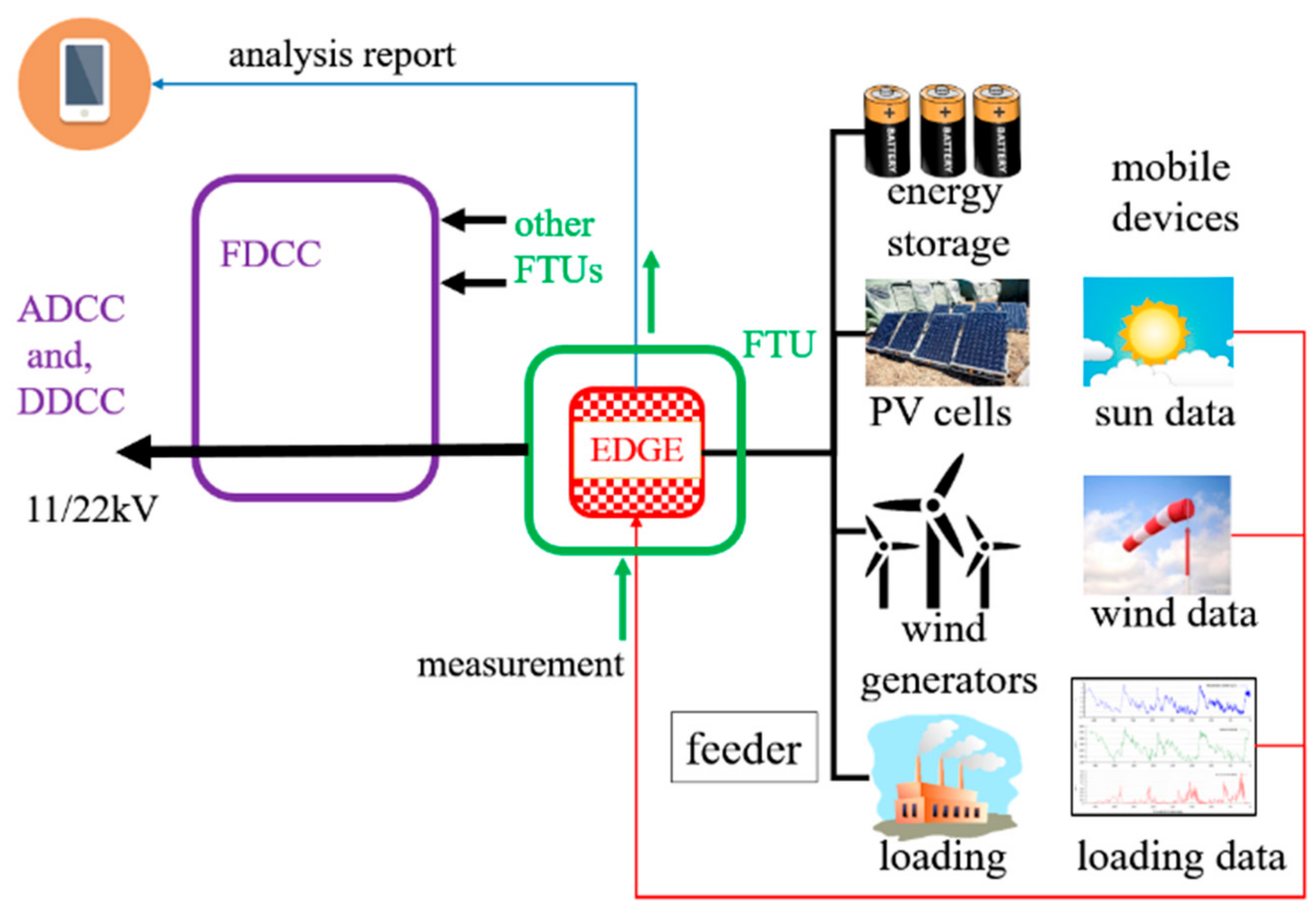
The feeder terminal unit (FTU), which is the distribution automation for smart operations of active distribution networks (ADNs) that are composed of distributed renewable energies and loads, measures the manner of power flow and sends it back to the Feeder Dispatch Control Center (FDCC) without further manipulation. Nowadays, the underlying standard functions of FTU are measurement, control, and fault detection [1]. However, the lack of analysis and computing capability is limited to ADN smart operations. In Figure 1, we present a novel EDGE with functions in a timely feeder status forecast, power flow analysis, important-factor explainer, and secured communication features inside a system-level platform.

The system is named EDGE because it works inside the FTUs, which are next to subscribers. FDCC collects and sends data to the Distribute Dispatch and Control Centre (DDCC) afterward. The results are shown on a mobile phone for localizing monitoring.

Some edge computation platforms of the hybrid renewal energy ADNs are discussed as follows. Kulkarni announced a similar concept, funded by the United States Department of Energy, to establish a situational awareness system [2]. This framework is named Global Asset Monitoring Management and Analytics. It contains functions of the power quality sensor, the Advanced Metering Infrastructure network, and the transformer sensor. After communicating data to a cloud server, mobile phones show their computation results. Its intelligence feature relieves the on-demand connectivity burden to centralized computation. Unfortunately, it is a low-cost platform, costing $4, without sufficient computation resource information.

Another study dispatched the reactive power control of the service-transformer by Moghe and Tholomier [3,4]. They presented the Edge of Network Grid Optimizer (ENGO) platform, attached next to the transformer chassis, that regulates the voltage by switched swarm capacitors. The cost and complexity of collecting all renewal energy utility situations and reporting to the FDCC become a challenge for rapid dispatch. A swarm of ENGO platforms, on the Omega feeder, inject the reactive power from the fixed capacitor bank to regulate the voltage variation.

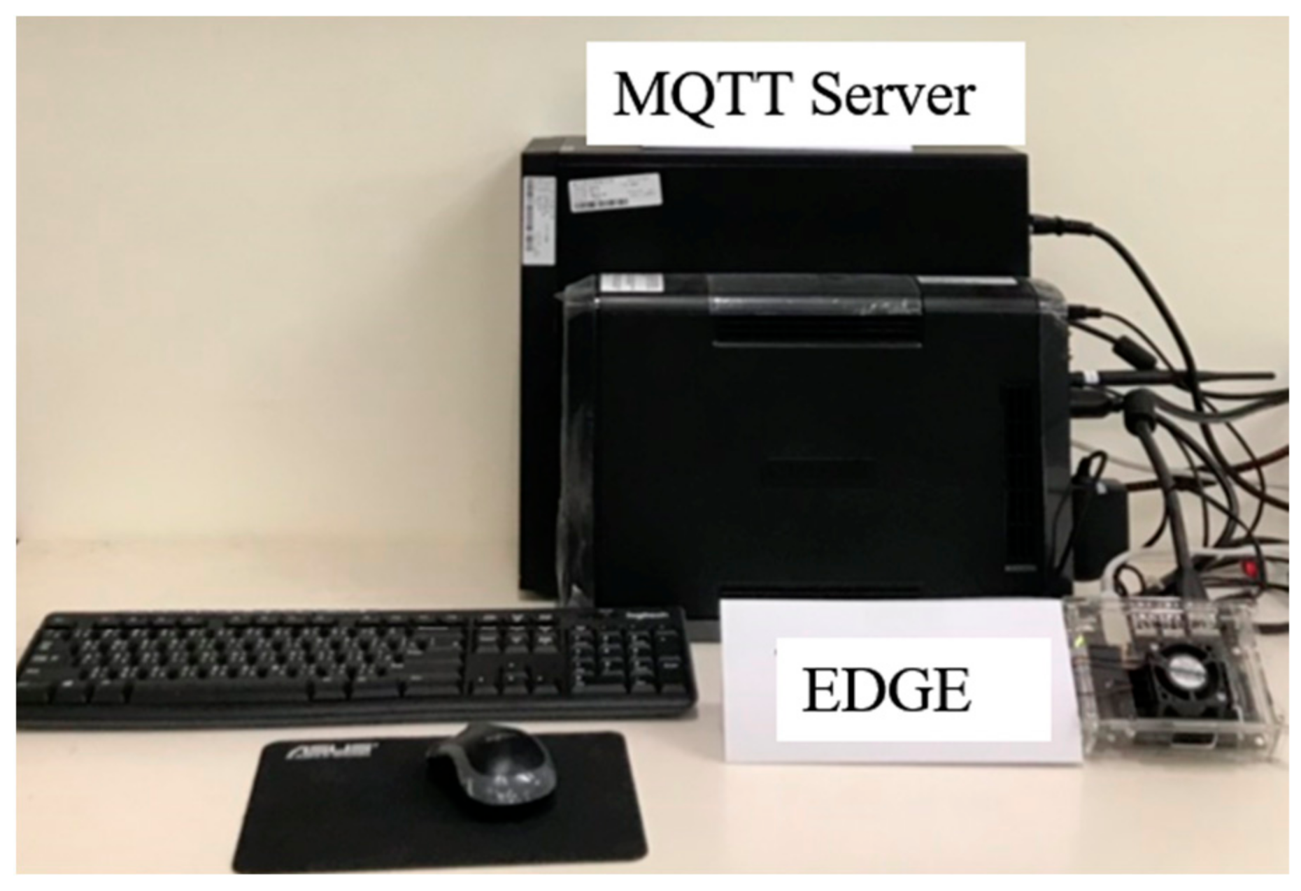
Thus, the proposed EDGE platform improves these features by using the new silicon technology chip and popular machine learning concepts. The platform has enhanced the function of the existing FTU, and offloads the FDCC computation work. Information on raw subscribers limits sharing to power generation and transmission companies by regulations. DDCCs or Area Dispatch and Control Centers may process the subscribers’ forecast work from many FTU terminals. This EDGE platform is designed to be handy in installation, and shares a centralized system risk. This paper presents a lab prototype concept allocated inside the FTU chassis in Figure 2.

Generally, in Taipower, each feeder has three FTUs, one distribution substation burden, and typically more than fifteen feeders. Therefore, more than 45 FTUs may serve in a distribution substation. This is not to mention that more than three distribution substations are in each DDCC or FDCC management district. If all these load data are sent to a local server in DDCC or FDCC to conduct an hour-ahead or 15-min-ahead forecast and compute the factors, the computing load becomes too heavy to complete within the allotted time. Consequently, EDGE is necessary to forecast the FTU [5] load data individually and to merely send the forecast results to FDCC to integrate all the information, and to make the correct or optimal decision. Furthermore, according to IEEE Std 1547.4-, distribution systems can be clustered into a number of microgrids to facilitate powerful control and operation infrastructure. Consequently, each FTU measurement area is planned as a microgrid, a feeder is divided into three microgrids in this paper for additional smart operations during normal operations or contingencies in the near future, and the multi-microgrid operation needs real-time computing without data transmission delay [5]. Accordingly, the development of edge computing in FTU is indispensable. The corresponding research is conducted in this paper.

Compared with a traditional microprocessor-based platform, the newly announced EDGE platform installs the machine learning package in the computer language, Python, and the corresponding acceleration circuit in its silicon chip. The cross-platform strength migrates high-level software stacks from personal computers (PCs) to EDGE without recompiling efforts. Thus, many available open-source software functions and researchers associate the work in different locations and different programming machines.

The long short-term memory (LSTM) method predicts power consumption [6]. Wang [7] proposed an EMD-PCA-RF-LSTM wind power forecasting model to improve the accuracy of wind power forecasting, and the experiment result indicates this model provides the most accurate results. Nevertheless, the trained model has no explanation of its important-factors association. A game-theory-based method, SHAP, parsed the LSTM models and arranged them in the graphical expression in this study. The Ngspice simulator is the power flow analyzer, and runs on EDGE’s distinctive CPU processor architecture [8]. Zhang [9] and Huang [10] investigated the transient analysis of the railway traction application in terms of the integration circuit elements under the personal computer environment. This concept inspires leverage of the Ngspice simulator as the power flow analyzer, and runs on the EDGE’s distinctive CPU processor architecture [8] and Linux operation system.

In communication, the message queuing telemetry transport (MQTT) protocol forms the parties of the EDGE, broker, and mobile phone applications. Finally, the SQLite system is the database archive that manipulates the real-time, historic, forecast, and analyzed data and images during service time. Accordingly, the significant blocks of the EDGE platform, which comprise the feeder forecast, power flow analyzer, important factor explainer, communication protocol, and database archive (SQLite), are proposed and shown in Figure 3.

Section 2 briefly presents the system design concepts with designated modules, including the LSTM model, power flow analyzers, and important-factor explainer functionalities. Section 3 exhibits the detail of each associated function in Section 4. Finally, the discussion and conclusion of each experiment are presented in Section 5.

2. System Design Concepts

This section presents the proposed system’s strengths, design constraints, and performance considerations.

2.1. Platform Introduction

The new Nvidia™ Jetson Nano (Santa Clara, CA, USA) device is chosen because of the low cost, Ubuntu operating system, 4 GB memory, 128 GB secure digital memory card (SD card), machine learning optimization package, and graphics processing unit (GPU) core features. The functions on the EDGE platform, which consist of different Python computer language (Python) packages for associating the five blue blocks, are seen in Figure 4. In this paper, we reconfigured and compiled several source files implemented into the EDGE platform as a computation engine. The complete computation platform software stack is shown in Figure 4.

2.2. Data Assimilation

The data assimilation process arranges the forecast data from the public weather service and power company. A government facility, Central Weather Bureau, offers weather information through the Opendata API mechanism. The operation information is obtained via DNP 3.0 [11,12] and IEC61850 [1] protocol using 4G or fiber media. Unfortunately, data sample time variation or missing content may cause the forecast solver to have trouble. Thus, the data assimilation process plays the role of compensation above practical drawbacks in some manners.

2.3. Forecast Solver

Information on the calendar, weather, and feeder operation act as the forecast solver’s input source and validation target. In contrast, the solver’s output build up the forecast model and the future feeder status, such as the voltage, current, and power. In the platform, the 128 numbers of the Maxwell^® cores host this forecasting work using the TensorFlow package. Under the limited memory space, the solver’s parameters and spending time are the major consideration during the development, which may impact its performance.

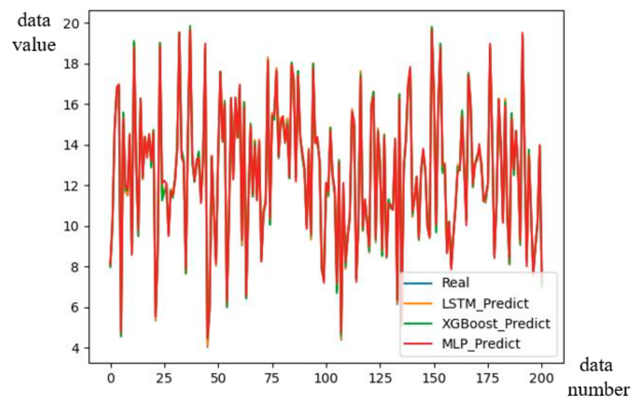
Newly announced time-series forecasting methods, such as the Arima [13], GlunoTS [14], and Fbprophet [15], simplify the forecast work on its merits. However, the method mixes all the time information into one data series, but not in the separated factors view. Two deep learning methods and a decision tree method are the Vanilla LSTM, and Multi-Layer Perceptron Model (MLP), and the eXtreme gradient boosting (XGBoost) as another forecasting approach. The XGBoost method is excellent due to its short model training time. However, it has the drawback of exhibiting slightly poor performance in terms of important-factor explanation accuracy from our test. MLP is good due to its short computation time and weight accuracy. However, the inherent vanishing gradient problem [1] resulted in the LSTM model being selected in this study.

In recent studies, the LSTM model for long-term, system-level load forecast has excellent performance [7,16,17]. In addition, the prediction error is acceptable for system operation. Dong investigated the LSTM and another popular machine learning method for long-term load forecast, demonstrating superior performance and great practicality [18]. Moreover, the LSTM model can be explained and can obtain its important factor. Pal applied the SHAP method for occupancy detection from energy consumption data [19]. The LSTM forecast solver, power flow analyzer, and important-factor explainer background are shown below.

As shown in Figure 5, a Vanilla LSTM network model has three gates: the forget gate, $f_t$; the input gate, $i_t$; and the output gate, $o_t$. The set of weight vectors, $\underset{¯}{w}$, includes the independent weights in the $w_f$, $w_c$, $w_i$, and $w_o$ notation [20,21]. The trained model includes the set of tuned weight vectors, $\underset{¯}{w}$, which the important-factor block investigates afterward.

The mathematical equations for the LSTM model are in Equations (1)–(6). Bias vectors are represented by the b_i, b_f, b_o, and b symbols. The additional memory cell candidate, ${\overline{c}}_t$, is used to add long-term memory via the activation function. The states, $C_{t-1}$ and $H_{t-1}$, refer to the previous state cell memory and the output, respectively.

$$i_t=\sigma \left(w_i{H}_{t-1}+U_i{X}_t+b_i\right)$$

(1)

$$f_t=\sigma \left(w_f{H}_{t-1}+U_f{X}_t+b_f\right)$$

(2)

$$o_t=\sigma \left(w_o{H}_{t-1}+U_o{X}_t+b_o\right)$$

(3)

$${\overline{c}}_t=\tanh \left(w_c{H}_{t-1}+U{X}_t+b\right)$$

(4)

$$C_t=f_t{C}_{t-1}+i_t{\overline{c}}_t$$

(5)

$$H_t=o_t\tanh \left(C_t\right)$$

(6)

2.4. Important-Factor Explainer

The important-factor explainer extracts the input forecast model, and demystifies the impact concerning the calendar and weather factors as the output. For example, the high-loading condition in the industrial area during the off-hours would be a safety issue or something else. A significant amount of computation work evaluates its contribution according to the factors’ permutation on the game theory concept. Hence, the four cores of the ARM CPU are responsible for this work, and deliver it to the next phase.

This feature elucidates the machine learning model into conceptual ideas regarding values for an explanation. Shawi [22] showed that the SHAP method is better than the Local Interpretable Model-agnostic Explanations (LIME) method and the Anchors method, with shorter computation time and proper identity disclosure. Thus, Lundberg [8,9,10] used the SHAP method in explaining the medical LSTM model in a graphical illustration.

From (1)–(6), it is a challenge to explain the important factor in the trained LSTM model. Therefore, a local and simplified model, $f\left(z\right)$, approaches the LSTM model, which tries to explain the factors under the forecast input case. A single unique solution to this explanation, proved by Lundberg [23], requires satisfaction with the three desirable properties in local accuracy, missingness, and consistency. A mapping linear regression model, $g\left(z\prime \right)$, represents to $f\left(z\right)$ by associating ${\varphi }_o$ and all ${\varphi }_i$ factors in (7) [23,24].

$$f\left(z\right)=g\left(z^{\prime }\right)={\varphi }_o+{\displaystyle \sum _{i=1}^k{\varphi }_i{z}_i^{\prime }}$$

(7)

Each factor, ${\varphi }_i$, contributes its individual merits, and satisfies the local accuracy property. In (7), where $z^{\prime }\in {\left\{0,1\right\}}^k$ for the simplified input information, ${\varphi }_i\in ℝ$ is the real numbers, and k equals to the 14 factors in this paper. The symbol, ${\varphi }_o$, denotes the model output when no inputs are available. In this paper, the symbol, ${\varphi }_i$, consists of the hourly important-factors result every 168 h. After normalizing the vector, ${\varphi }_i$, the important-factor value in each factor under the hourly forecast work.

Fair evaluation is a complex problem when the forecast model owns many factors. The Shapley value [25] aims to understand the cost or gain between collaborating factors based on the contribution term in the cooperation action. In other words, the factor with the higher Shapely value dominates the coalition-winning possibility. For example, more gold components inside the same alloy volume would be heavier than others. From the Narahari [26] and Kolker [25] press, the (8) Shapley value, $S{h}_k$, for each factor (not important factor), is shown as the following:

$$S{h}_k={\displaystyle \sum _{s\subset n}\frac{\left(s-1\right)!\left(s-n\right)!}{n!}\left(V\left(s\right)-V\left(s-k\right)\right)}$$

(8)

The symbol, s, denotes the number of a factor in the coalition, s; k denotes the cooperation members in a group. The symbol, n, represents the group number. Multiplying all of the possible coalitions $\left(s-1\right)!\left(s-n\right)!$ and marginal contributions $\left(V\left(s\right)-V\left(s-k\right)\right)$ with a summation of them together, the Shapley value vector is obtained by dividing the permutation number, n!.

Later, the Shapley value vector is transferred into the SHAP format to obtain the important-factor data in the format of the (7) [23]. Further discussion of the properties in terms of local accuracy, missingness, and consistency stands for the intuitive view of the SHAP result.

2.5. Power Flow Analyser

Regardless of the forecast solver accuracy, the result cannot satisfy electrical theory and cover all nodes’ data. Thus, analyzers initially convert equivalent loading parameters from the forecast results, and then compute the feeder behavior with practical parameters. The expected items include line loss, neutral line voltage, and loading status.

Available power flow computation packages are listed in Thurner [27]. After evaluation, the pandapower (2.1.0) and pydgrid (0.5.2) packages cannot complete the test routine in the EDGE environment. The PYPOWER (5.1.4) package runs perfectly, but does not support several scenarios in the transient analysis. Finally, the analyzers’ computation engine is built by ngspyce (0.1), and re-compiled by the Ngspice engine. Python renders the user-interface images from Ngspice’s result in floating number matrices. This tool, Ngspice, is involved in the very large-scale integration clock signaling simulation [28] and the new CPU accelerator design [29] to prove its correctness.

The time-step value settings define the voltage node memory consumption in the transient state simulation. In a 138.89 µs time-step case, each voltage vector occupies 46,144 bytes within an 800 ms simulation period, consisting of the 5768 elements in the float64 data format of Python (92,288 bytes). Thus, a large-scale fault case simulation is not suitable for placing in the EDGE process, but rather the workstation machine.

2.6. Database Archive System and Communication to Remote Device

The important-factor explainer and power flow analyzer blocks generate the numerical data and images from the trained LSTM model. Later, real-time data are saved into the database first and fetched to the forecast solver to update the LSTM model. By moving the time window, it periodically publishes information to the broker. A comprehensive and secure database archiving file system offloads the design effort and supports the encryption function, as shown by Wang [30]. The EDGE uses the open-source SQLite database controller to store the values, strings, and images. During the operation, both the Maxwell^® and ARM core access the SQLite database simultaneously, and leave the low-level control work by the Python package.

Next, we propose quality and low-cost methods for communicating the EDGE, broker, and user’s remote devices. A private MQTT broker on a regular PC, which is a product of HiveMQ^®, handles all the subscribed and published events via the internet. The MQTT method supports Quality of Service to ensure communication integrity [31,32]. The transport layer security (TLS) communication protocol ensures security requirements. The application, MQTT Dash^®, is available for download on Android mobile phones to monitor feeder status anytime and anywhere.

3. Implementation

This section introduces the systematic implementation of the aforementioned blocks on EDGE, MQTT broker server, and mobile users. To inhibit real subscribers’ information, Equation (9) simulated its power factor, $p{f}_{a,b,c}^{*}$, concerning the load current, $i_{load}$, trend in Figure 6:

$$p{f}_{a,b,c}^{*}=0.75-\left(88i_{load}-10.7i_{load}^2+0.075i_{load}^3\right)\times {10}^{-5}$$

(9)

3.1. Forecast Solver

A forecast solver sequentially runs the LSTM network and cascaded processes (Figure 7). The forecast models of the input sources, such as date, atmosphere, and sunshine, are provided in historical and real-time views. From the power company, ten items of historical data predict the feeder voltage, $v_{a,b,c}$; current, $i_{a,b,c,n}$; and assumed power factor, $p{f}_{a,b,c}^{*}$. Thus, the forecast feeder voltage, ${\widehat{v}}_{a,b,c}$; current, ${\widehat{i}}_{a,b,c,n}$; and the power factor, ${\widehat{pf}}_{a,b,c}$, are determined at the end.

The data sources of the identified factors are listed as follows: year (2019–present), month (1–12), day (1–31), weekday (1–7), hour (0–23), station pressure (hPa), temperature (°C), relative humidity (%), wind speed (m/s), wind direction (360°), sunshine hour (h), global radiation (MJ/m²), visibility (km), ultraviolet index (none), and cloud amount (0–10).

The normalized process compresses all data into the range of 0–1 to unify the variables’ inherent magnitudes. After that, the reshape to tensor block packs the 2D data into the tensor format following the batch size setting, and then copies them to the important-factor explainer. A validation process verifies the trained model’s performance in terms of the loss function with the training dataset, which evaluates the batch size, LSTM unit weight, and epoch number setting. The denormalization process obtains the forecast result from the introduced estimation estimated model and external forecast data. Thus, in every epoch routine, the entire dataset is driven forward and backward through the LSTM network to update the weighted vectors. Lastly, the trained models save the files. This LSTM network repetitively updates the trained model in the next forecast slot. Finally, six images of the voltage, current, and power flow estimation are stored in the database archive for the mobile device application.

3.2. Important-Factor Explainer

As the previous section discussed, the SHAP package explains the important factor, ϕ_i., of the LSTM model. This process consumes the most resources, computation time, and memory due to the LSTM input tensor size. If the batch size parameter is 12, then the size of the input tensor is 6,756,480 bytes in this study. Only 40% of the input tensor data is used to meet EDGE memory space limitations in this work.

Temporally, the hourly forecast model contains the updated LSTM model, calendar, and weather information in the 168 h time length. Later, the important-factor explainer elucidates this model and carries on the local survey. For example, the effect of the unregistered and photovoltaic cell facility apparatus may be coherent with the cloud amount factor from the explanation work. Then, EDGE communicates to the feeder dispatch control center for the corresponding strategy.

3.3. Power Flow Analyzers

As shown in Figure 8, the Ngspice program is configured by following the instructions in the user’s manual [33]. Then, to convert the Ngspice as a shared library (.so) file for Linux kernel assertion, a parameter adjustment process computes the load model, Z_load, values and adjusts the SPICE model. By converting the loading’s passive component values from the forecast power, P; reactive power, Q; and currents, transient-state simulation is executed to derive the concerned neutral line voltage and current in vector format. Thereafter, a few trigonometric functions are converted to symmetrical components. Fast Fourier transform analysis is conducted to compute the harmonics of any vector and compose them into images. Another steady-state analysis provides the node voltage or current in the designed frequency point. This analysis saves memory and computation time compared with transient-state analysis. The P and Q values in each hour are computed and presented in the image file format.

The topology of DNs is generally complicated. Therefore, the simplified feeder model, which is composed of an equivalent feeder, is connected with its load. Consequently, a complicated feeder with various types of load and renewable energy can be simplified, as shown in Figure 9.

This was proposed due to the fast calculation of the feeder voltage profiles and losses [34]. Furthermore, three FTU units typically measure phase voltage, $v_{a,b,c}$, and line current, $i_{a,b,c,n}$, in the feeder. The known primitive impedance Z-matrix $\left[Z_{1,2,3}\right]$ of an equivalent feeder section is determined from its operation. Some power system elements are converted into the SPICE model [35,36], and others are converted into the simplified model. The neutral line resistance, $R_{Z3}$, and inductance, $L_{Z3}$, are added to evaluate the concerned current.

Figure 10 shows the single-line diagram of a real distribution feeder of Taiwan Power Company (TPC). The simplified feeder models proposed in [22] represent the end voltage and line loss calculations of each line section. First, the transformers with their loads or distributed renewable energies (DREs) in each lateral were lumped to the bus of a three-phase, four-wire feeder main, and then the transformers and their loads can be integrated and simply represented by their equivalent loads, as shown in Figure 11 [28]. The partial feeder in each FTU measurement area can be represented, as shown in Figure 12. Finally, the equivalent length and loads of the simplified feeder model for the end voltage or line loss calculations can be obtained by the formula derived in [22]. The simplified feeder models have been applied for simplified power flow computing to obtain bus voltage profiles and line losses with negligible error in unbalanced distribution feeders. Therefore, the simplified feeder models are used in this paper to build the circuit model in the simulation program with the integrated circuit emphasis (SPICE) model for fast calculation with a doubtless convergence problem.

3.4. Database and MQTT-Communication

In general, the database stores the number of hours of data (5448) in three dedicated SQLite tables for the different feeder line conditions. The SQLite package handles most low-level work in negotiating the Linux file system. The rich database commands achieve the requirement in the merits of its database characteristic. SQLite can also be updated to the encrypted version using CryptSQLite, as demonstrated by Wang [30].

The MQTT system demonstrates the EDGE features. The interoperability of the SQLite and MQTT packages was implemented by Kodali [37]. The installation guide and software code are available on the HiveMQ^® website. The MQTT protocol features the quality-of-service levels, guaranteeing data transaction integrity. The broker supports the TLS/secure socket layer feature [15] to protect the secret with a private key. In EDGE, a software timer periodically publishes image files to the broker every 30 s.

The MQTT broker setup is straightforward concerning its instructions. The private key to enable TLS security is necessary, but not the central scope of this study. Protecting this broker machine in a secured location is highly recommended. Thereafter, the MQTT-Dash application would provide the landscape view of the important-factor image in Section 4.3.

4. Experiment and Discussion

The associated blocks of the forecast solver and important-factor explainer are examined. These blocks are the cornerstone in conducting a system-level experiment. Thereafter, a running EDGE device, a private MQTT broker server (Figure 13), and a few mobile phone devices from the system are utilized. Software performance indices and hardware operation characteristics present the results in this section.

4.1. Forecast Solver Performance Examination and Comparison

A total of 4704 rows (27 weeks) of historical data are used to predict the result of 168 sets (1 week). Each row and set contain 20 inputs and 10 outputs, respectively. A basic Vanilla LSTM model performs each forecast routine within 236 s with a batch size of 12, an LSTM unit of 64, and epoch times of 15. The mean absolute percentage error (MAPE) value verifies the work in (10):

$$MAPE\left(\%\right)=\frac{1}{168}{\displaystyle \sum _{i=1}^{168}\left|\frac{y_i-{\widehat{y}}_i}{y_i}\right|}$$

(10)

The consumption times and MAPE values are summarized in

Table 1. Forecast solver’s MAPE result in each FTU.

FTU	FTU1			FTU2			FTU3
Phase	A	B	C	A	B	C	A	B	C
voltage	0.4	0.4	0.5	0.4	0.5	0.5	0.5	0.5	0.5
current	17.0	21.3	24.5	12.1	14.6	15.9	13.1	14.3	15.4
P	21.3	26.8	31.6	14.9	18.0	19.6	16.1	17.5	18.9
Q	9.6	13.4	13.3	4.5	5.8	5.3	4.9	5.4	5.8
LSTM training time	495.9			484.4			485.7

Forecast period: 13 h (2184 time-series data), unit: % and sec.

. The consumption time takes an average of 488.6 s in LSTM training. The average MAPE values of voltage; current; real power, P; and reactive power, Q, are 0.46, 16.47, 20.52, and 7.56, respectively.

A forecast waveform in the FTU3 (phase A current) is presented in Figure 14. From the waveform view, the predicted and real are similar in the 168 h. The average MAPE values are 12.81%.

Next, we compare the important-factor performance under the LSTM, XGBoost, and MLP forecast solver. Equation (11) generates data value in every $d$ number following the randomized value, $R_n$, multiplying the preset weight values, $w_n$. From the preset weight, $w_n$, and randomized values, continuous serial data are adopted to examine the important-factor explainers’ performance. The candidate explainers involved two works: predict the data value (Figure 15), and benchmark the computed important factors (

Table 2. Important-factor explainer performance comparison of the LSTM, XGBoost, and MLP.

	$\mathbf{Nominal} \mathbf{Weight} {\mathit{w}}_{\mathit{n}}$	LSTM	MLP	XGBoost
$w_1$	0.02	0.02	0.01	0.00
$w_2$	0.12	0.12	0.10	0.04
$w_3$	0.20	0.18	0.19	0.11
$w_4$	0.29	0.31	0.32	0.26
$w_5$	0.37	0.37	0.38	0.59
run time (sec)	-	46.90	1.22	46.23

Preset weight values, $w_n$ are 0.05, 0.30, 0.50, 0.75, and 0.95.

).

$$f\left(d\right)={\displaystyle \sum _{i=1}^5{R}_n\cdot w_n}$$

(11)

4.2. Important-Factor Explainer in the Polynomial Equation Case

In a trained model, the important-factor explainer identifies the important factors, ${\varphi }_i$, and compresses them into a per-unit level. The parameters of this test LSTM model are identical, to review its settings. As shown in

Table 3. Important-factor explainer performance in the polynomial equation case.

	$\mathbf{Nominal} \mathbf{Weight} {\mathit{w}}_{\mathit{n}}$	LSTM ${\varphi }_i$
$w_1/{\varphi }_1$	0.02	0.02
$w_2/{\varphi }_2$	0.04	0.04
$w_3/{\varphi }_3$	0.05	0.05
$w_4/{\varphi }_4$	0.07	0.08
$w_5/{\varphi }_5$	0.09	0.07
$w_6/{\varphi }_6$	0.11	0.12
$w_7/{\varphi }_7$	0.13	0.12
$w_8/{\varphi }_8$	0.15	0.15
$w_9/{\varphi }_9$	0.16	0.16
$w_{10}/{\varphi }_{10}$	0.18	0.18

, the comparison between the nominal weight, $w_n$, and important factor, ${\varphi }_i$, are shown in the 10 steps in the 4704 input data rate.

4.3. System Manipulation

Table 4. Computation time comparison on EDGE and PC.

Platform (FP16 Performance (TFLOPs))	EDGE Nano Jetson (0.472)	PC i7-5820K CPU P2000 GPU (3.0)
LSTM forecast LSTM networks	1679.6	413.5
LSTM forecast estimation	92.2	22.0
Symmetric component analysis	6.8	1.3
Steady-state analysis—line loss	17.1	3.1
Important-factor explainers	2932.4	530.1
MQTT publish	15.4	3.0
Total (seconds)	4743.5	963.0

The term, FP16, refers to the “16-bit floating point”.

summarizes the computation time in the EDGE and PC environments. The different FP16 performance indices hint at the reasonable computation time in the selection of the new tensor processing unit (TPU) platforms. The proposed EDGE, with a score of 0.472, spends 4743.5 s in one routine. The PC platform is faster with richer resources.

Another result is the communication burden breakdown list in all classifications, as presented in

Table 5. Communication burden review.

Data	Source	Classification	Protocol	Burden
feeder	FTU	historical	database	--
weather/solar	CWB	historical	database	--
weather/solar	CWB	observation	web API	2.58 k/h
feeder	FTU	measurement	database (IEC61850)	--
analysis result	EDGE	forecast	MQTT	467 k/h
weather/solar	CWB	forecast	web API	56 k/day

Unit: bytes; web API: the open weather data service from the Central Weather Bureau in Taiwan.

. Taiwan’s Central Weather Bureau (CWB) offers free weather and solar observation data hourly via the web application programming interface (API) in 2.58 kB. Each analysis result from EDGE converts to the images in 467 kB. The MQTT protocol is divided into many transmission control protocol layer packages in 1494 bytes. The daily CWB forecast data are 56 kB. Historical data and FTU measurement data are still from the TPC and CWB database in this study.

Figure 16 contains 15 importance factor analyses in the FTU3 current mode analysis; the hour and cloud importance factors are dominants. The high cloud, low wind speed, and low wind direction factors prove that the FTU3 feeder connects some PVs, but no wind energy generators are shown in the illustrations in Figure 6. Three-phase loading is almost in balance, except the B-phase is slightly higher.

The forecast result example is illustrated in Figure 17, which contains the PQ power, voltage, current, and transmission line loss manners. The white and gray color areas represent the day and nighttime, respectively. The dual vertical axes, start and end time, and legend form the necessary references from the small mobile phone screen view. A user client refers to a mobile phone and monitors feeder operation. The MQTT-Dash application subscribes to the desired topics and receives the latest images.

A running EDGE, MQTT broker, and mobile phone device form the proposed service. At a room temperature of 20 °C, EDGE and its system on a chip (SOC) consume power at approximately 17.6 and 9.0 W, respectively. The semiconductor’s junction temperature increases to 25 °C from the report on the Linux kernel [38]. Deploying EDGE outdoors may have a suitable thermal design margin during summer at 45 °C, but may not reach the operation limitation of 97 °C.

5. Conclusions

This study demonstrated an FTU-based feeder power forecast using the EDGE platform. This platform consists of data collection, forecast solver, important-factor explainer, power flow calculation, MQTT publisher, MQTT broker, and MQTT-Dash application. Theories were introduced from the algorithm equations to implement strategies to build up the system.

The forecast solver result indicated the waveform comparison between the real and forecast outcomes in approximately 488.6 s. The important-factor explainer examined the design concept, and its normalized factors exhibited a 6.54% error.

In the system experiment, the values of surface temperature, junction temperature, and power consumption performed well within the Jetson Nano SOC IC specification. The user client application displayed EDGE’s published images from the MQTT broker service. All of the images, forecast data, analyzer output, and loss tables were stored in an SQLite format file in an SD card for further application. The developed prototype platform could be implemented in FTU in the laboratory to enhance the intelligence function in smart ADN operations.