Finite Difference Modeling of the Temperature Profile during the Biodrying of Organic Solid Waste

Abstract

Biodrying is a complex process that is very useful in the treatment of solid waste, where variables, such as temperature, thermal conductivity and the moisture content of organic matter, oxygen concentration in the pore space of the waste mass, microbial heat generation, microbial biomass, among others, are involved. Given this complexity, the development of mathematical models that help us to understand this bioprocess is fundamental. In the present work, a mathematical model, based on the finite difference method, was developed to predict the temperature profile at nine recording points, in an organic solid waste pile, during the biodrying process. The bioprocess was carried out under natural convection and solar radiation conditions, inside a greenhouse-type structure. A network of 5³ nodes, distributed in the x, y and z directions, on a rectangular prism, was developed. From this network, 27 base nodes were taken and the energy balance was developed for each node, and with this, the equation was obtained, in explicit form, to calculate the temperature. In these base equations, the microbial heat generation was considered, at between 2 and 140 W/m³; the convective coefficient was between 1 and 5 W/m² °C; and the daily records were taken inside the greenhouse for the solar radiation (0 to 450 W/m²), temperature (15 to 50 °C) and RH% (70 to 30). The modeled temperature profiles of the center (C) and the midpoints of the pile were, on average, 91% close to the experimental values, during the period from 0 to 20 days of biodrying; 70% close, during the period from day 21 to 35, the period when the modeled values were lower, due to the turning of the pile; and 94% close to the experimental values from day 36 to 50, when the modeled values were higher, also due to turning. The modeled temperature profiles of the left, right, upper and lower surfaces were, on average 92% close to the experimental profiles over the 0–35 day period, and the modeled and experimental values were practically identical from day 36 to 50 of the biodrying process.

1. Introduction

Biodrying is used to reduce the moisture content of different types of waste, to produce refuse-derived fuel. Among the wastes that have been tested, are municipal solid waste [1], food waste [2,3], agricultural and agro-industrial waste [4], among others. During biodrying, the successful development of the thermophilic phase is fundamental to achieve a more efficient process where the greatest amount of water in a short time is removed. There is an important relationship between water removal and bioheat generation, a high matrix temperature and air flow, as reported by Xin et al. [3]. For modeling the thermal behavior of a biodrying pile, the different heat transfer mechanisms that take place in this bioprocess must be studied in detail, namely the heat received from the solar radiation, the exothermic heat generated by the metabolic activity of the aerobic microorganisms, and the heat lost or gained through the convection–conduction, added to which the depth and location of the recording point should also be taken into consideration [5,6,7], so that the temperature differences observed in the temperature profiles would be the result of the thermal balance between these phenomena [8].

Mason [9,10] carried out a comparison of the models developed up to that date, in order to show which of them generates better results, compared to the experimental data, but all of the models study the composting process.

In the studies carried out by Vlyssides et al. [11], Guardia et al. [12], Petric and Selimbasic [13] and Zhang et al. [8], the mathematical models used are presented and then the modeled results are compared with the experimental data, obtaining, in most of the composting process, a degree of closeness of 70 to 80% with the experimental data; it should be noted that in none of these works, was a quantification carried out of the microbial growth, which in turn causes internal heat generation.

To date, very little work has been carried out on the modeling of the biodrying process. Díaz Megchún [14] worked on the modeling of the heat transfer in one dimension, to predict the behavior of the temperature, but only in the center of the pile, achieving unsuccessful results. Lawrance et al. [15] developed a mathematical model of the mass balances of the batch biodrying of municipal solid waste. Lawrence et al. [16] also worked on a model and simulation of food waste biodrying, where an attempt was made to develop mass and energy balances, using the first principles to predict the variation of the key variables, namely the concentration of degradable matter, moisture, oxygen concentration, and temperature, based on the process kinetics. Both models [15,16] were developed for reactors.

Orozco et al. [17] worked on the modeling of biodrying. Although this work also focused only on the center of the pile, they reported several interesting conclusions, including their determination that part of the metabolic heat is used to raise the temperature of the pile, and that practically all of the energy for the biodrying of the pile is provided by the ambient convection and solar radiation, but that the drying rate is accelerated by the high values of the wet bulb temperature, caused by the microbial heat. Because of this, the need arose to develop a mathematical model that would be able to predict the temperature profile at any point in a waste pile, with the biodrying carried out under natural convection and solar radiation conditions inside a greenhouse-type structure.

The few articles published on the modeling of biodrying have only focused on the modeling of the center of the pile and in a single direction or dimension (pile height). Therefore, the aim of the present work was to develop a mathematical model, based on the finite difference method, which would allow three-dimensional modeling [18,19,20] in order to predict the temperature profiles during biodrying, at the different recording points of an organic solid waste pile and, therefore, at any x, y, and z coordinate point where the temperature sensors were placed inside the pile.

2. Materials and Methods

2.1. Source of Data

We worked with the same experimental data reported by Díaz Megchún [14] and also used by Orozco et al. [21]. In both studies, the evolution of the thermal behavior of several biodrying piles was described, and particularly the temperature of the pile analyzed in the present work, started at 25 °C and rose to 65–70 °C in ten days, then from day 11 to 35, it slowly dropped from 65 to 30 °C, and from then until day 50 it fell even more slowly, until it equaled the ambient temperature that was between 23–25 °C (Figure 1 and Figure 2).

The overall process can be divided into two stages: (a) the biodrying plus ambient drying stage (with a duration of 36 days), and (b) the ambient drying only stage (with a duration of 14 days). It can be seen that the center and inner layers of each pile (C, Lm, Rm, Bm, Um) recorded the highest temperatures, followed by slightly lower temperatures for the base (B) surface, then for the upper (U) surface with very pronounced temperature extremes (highs and lows), and, finally, with the lowest temperatures recorded on the lateral faces (L and R), which had moderate temperature extremes.

Regarding the environmental conditions inside the greenhouse-type structure, the temperature and relative humidity varied during the day from 47–50 °C and 18–22%, respectively, while at night they ranged from 13–15 °C and 77–80%, respectively.

2.2. Considerations for the Heat Transfer and Microbial Heat Generation

For each heat transfer mechanism and microbial heat generation, which, in addition to the environmental conditions inside the greenhouse (convection) depended on the position of the pile in the greenhouse (solar radiation), their expressions, reported in the specialized literature, were researched and selected. The base differential equation for the heat transfer is presented below, in rectangular coordinates and in the x axis direction [22,23].

$$\frac{1}{\alpha }\frac{\partial T}{\partial t}=\frac{{\partial }^{2}T}{\partial x^2}+\frac{\dot{e}}{k}$$

(1)

The above is the basic unsteady state heat transfer equation, which can easily be extended to three dimensions (by adding the terms $\frac{{\partial }^{2}T}{\partial y^2}+\frac{{\partial }^{2}T}{\partial z^2}$) [24,25]. This basic equation can be expressed in finite differences, for the internal node 1, in a volume element and with nodes 0 and 2 on both sides in the x direction, as follows [26]:

$$\frac{1}{\alpha }\frac{\left(T_1^{i+1}-T_1^i\right)}{\Delta t}=\frac{T_0^1-2T_1^i+T_2^i}{\Delta x^2}+\frac{e_1^i}{k}$$

(2)

This same expression could be obtained by applying an energy balance to the volume element and considering that the heat flow by conduction, is from nodes 0 and 2 to node 1 [27]:

$$\rho A\Delta x cp \frac{\left(T_1{}^{i+1}-T_1^i\right)}{\Delta t}=kA \frac{\left(T_0^i-T_1^i\right)}{\Delta x}+kA \frac{\left(T_2^i-T_1^i\right)}{\Delta x}+e_1^{i}A\Delta$$

(3)

By multiplying by $\frac{1}{A\Delta xk}$ and then substituting $=\frac{\mathrm{k} }{\mathsf{\rho } \mathrm{Cp}}$, the same expression is obtained:

$$\frac{1}{\alpha }\frac{\left(T_1^{i+1}-T_1^i\right)}{\Delta t}=\frac{T_0^1-2T_1^i+T_2^i}{\Delta x^2}+\frac{e_1^i}{k}$$

(4)

From the latter, by rearranging and substituting $\alpha \frac{\Delta t}{\Delta x^2}=\tau$, the explicit expression for determining the temperature for node 1 was obtained:

$$T_1^{i+1}=T_1^i\left(1-2\tau \right)+\tau \left[T_0^i+T_2^i+e_1^i\frac{\Delta x^2}{k}\right]$$

(5)

What has just been shown is that to obtain the temperature expressions at any node, one has to start with an energy balance, where the sum of the heat flows from all directions will be towards the node in question, and then obtain, in explicit form, the temperature equation. Thus, this principle was the foundation of the present work, as it was for Cengel and Ghajar in a study reported in 2011 [28].

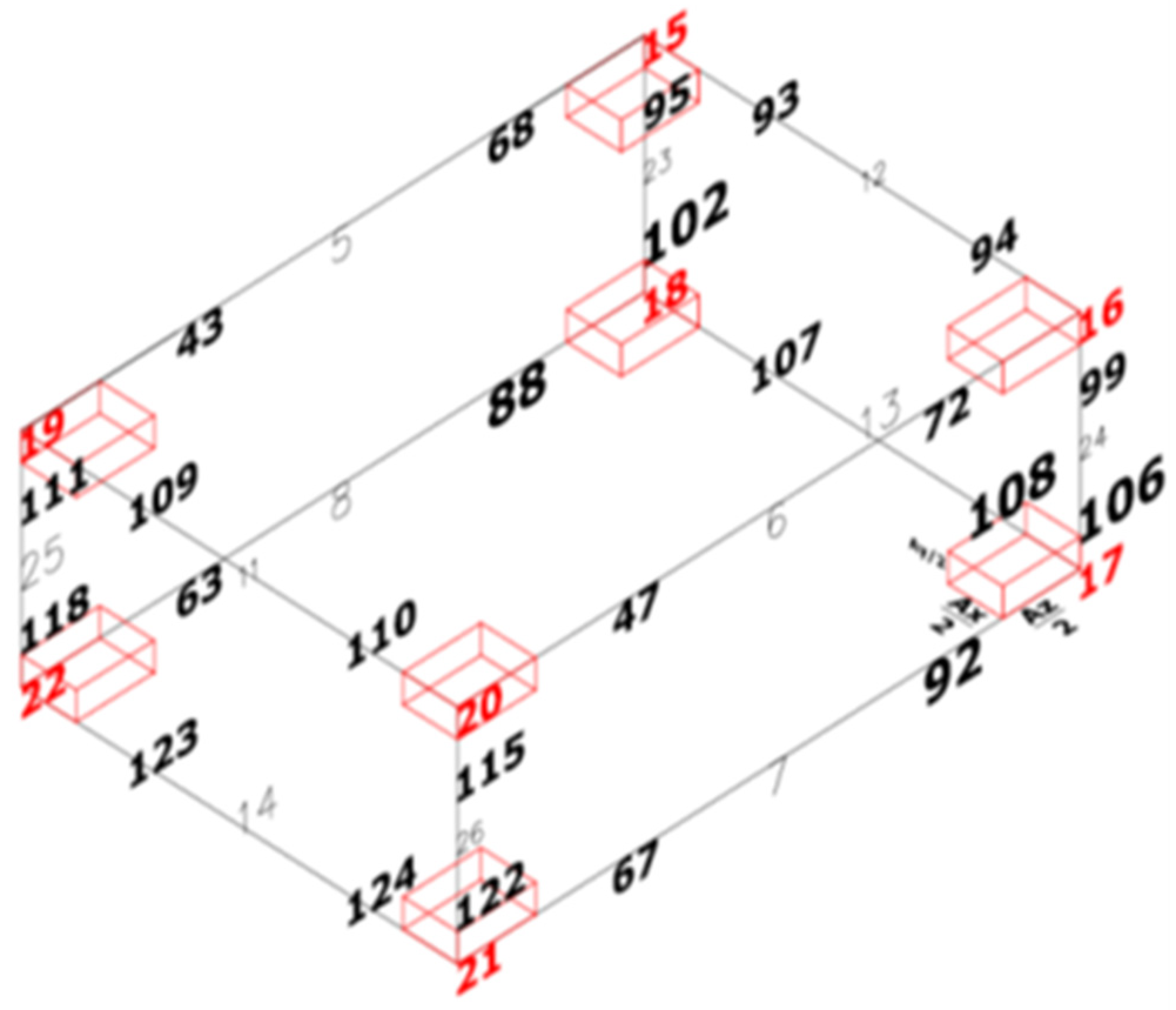
2.3. Distribution of the Node Network

Thus, Figure 3 presents a scheme with the distribution of the 27-node base network on a rectangular prism, as a geometric approach to the pyramidal pile reported in the work of Díaz Megchún [14], since it presents the same volume to surface area ratio. From this figure, the nodes can be classified as an interior node (1), surface nodes (six: 0, 2, 3, 4, 9 and 10), edge nodes (twelve: 5, 6, 7, 8, 11, 12, 13, 14, 23, 24, 25 and 26) and vertex nodes (eight: 15, 16, 17, 18, 19, 20, 21, and 22).

To determine the energy balance at each node, and thus to start the development of the equations, it is necessary to “visualize” the volume element, the node number and the “boundary cut” that the volume element will have at each of the x, y and z axes, resulting from the orientation of each of the faces or surfaces of the pile, which is shown in Figure 4.

In turn,

Table 1. Cuts and perpendicular areas for developing the energy balance for each node type.

Node Type	Node Number	Cut of the Volume Element at the Boundary	Areas Perpendicular to the x, y, z Axes
			x Axis	y Axis	z Axis
Internal	1	None	$\Delta y·\Delta z$	$\Delta x·\Delta z$	$\Delta x·\Delta y$
Surface	0 and 2	$\frac{\Delta x}{2}$	$\Delta y·\Delta z$	$\frac{\Delta x}{2}·\Delta z$	$\frac{\Delta x}{2}·\Delta y$
	3 and 4	$\frac{\Delta y}{2}$	$\frac{\Delta y}{2}·\Delta z$	$\Delta x·\Delta z$	$\Delta x·\frac{\Delta y}{2}$
	9 and 10	$\frac{\Delta z}{2}$	$\Delta y·\frac{\Delta z}{2}$	$\Delta x·\frac{\Delta z}{2}$	$\Delta x·\Delta y$
Edge	5, 6, 7, 8	$\frac{\Delta x}{2}; \frac{\Delta y}{2}$	$\frac{\Delta y}{2}·\Delta z$	$\frac{\Delta x}{2}·\Delta z$	$\frac{\Delta x}{2}·\frac{\Delta y}{2}$
	11, 12, 13, 14	$\frac{\Delta y}{2}; \frac{\Delta z}{2}$	$\frac{\Delta y}{2}·\frac{\Delta z}{2}$	$\Delta x·\frac{\Delta z}{2}$	$\Delta x·\frac{\Delta y}{2}$
	23, 24, 25, 26	$\frac{\Delta x}{2}; \frac{\Delta z}{2}$	$\Delta y·\frac{\Delta z}{2}$	$\frac{\Delta x}{2}·\frac{\Delta z}{2}$	$\frac{\Delta x}{2}·\Delta y$
Vertex	15, 16, 17, 18 19, 20, 21, 22	$\frac{\Delta x}{2}; \frac{\Delta y}{2}; \frac{\Delta z}{2}$	$\frac{\Delta y}{2}·\frac{\Delta z}{2}$	$\frac{\Delta x}{2}·\frac{\Delta z}{2}$	$\frac{\Delta x}{2}·\frac{\Delta y}{2}$

presents the 27 nodes of the basic network with the information about the cut of the volume element at the boundary and the heat transfer areas that must be taken into consideration for the three directions, or the dimensions for each type of node.

3. Results

3.1. Development of the Equations in Explicit form for Determining the Temperature at Each of the Nodes

The development of the equations for the nodes (numbers in Figure 5) of a rectangular prism of average dimensions, h = 0.65 m, BL = 2.0 m and BW = 1.4 m, was established from Figure 5, which corresponded to the location of the temperature sensors (letters) in the pile during the biodrying.

There were five nodes per direction (x, y, z) requiring 5³ = 125 nodes and therefore the same number of equations were developed. The separation between the nodes was calculated as follows:

$$\Delta \mathrm{x}=\frac{\mathrm{BW}}{\left(5-1\right)} ; \Delta \mathrm{y}=\frac{\mathrm{h}}{\left(5-1\right)} ; \Delta \mathrm{z}=\frac{\mathrm{BL}}{\left(5-1\right)} ;$$

(6)

The following relationships were also established to facilitate obtaining the equations: $\mathrm{a}=\frac{\Delta \mathrm{z}}{\Delta \mathrm{y}} ; \mathrm{b}=\frac{\Delta \mathrm{x}}{\Delta \mathrm{y}}$; once the above was established, the development of the model equations began.

Node 1 (sensor C).

As an interior node, it only receives conduction heat transfer [29] through all of the nodes adjacent to it (Figure 6): 34, 35, in x direction; 31, 38, in y direction and; 55, 80, in z direction. Therefore, the corresponding energy balance was:

$$\begin{array}{cc}\hfill \mathrm{k}\Delta \mathrm{y}\Delta \mathrm{z}\frac{\left(T_{34}^i-T_1^i\right)}{\Delta \mathrm{x}}& +\mathrm{k}\Delta \mathrm{y}\Delta \mathrm{z}\frac{\left(T_{35}^i-T_1^i\right)}{\Delta \mathrm{x}}+\mathrm{k}\Delta \mathrm{x}\Delta \mathrm{z}\frac{\left(T_{31}^i-T_1^i\right)}{\Delta \mathrm{y}}\hfill \\ \hfill & +\mathrm{k}\Delta \mathrm{x}\Delta \mathrm{z}\frac{\left(T_{38}^i-T_1^i\right)}{\Delta \mathrm{y}}+\mathrm{k}\Delta \mathrm{x}\Delta \mathrm{y}\frac{\left(T_{55}^i-T_1^i\right)}{\Delta \mathrm{z}}\hfill \\ \hfill & +\mathrm{k}\Delta \mathrm{x}\Delta \mathrm{y}\frac{\left(T_{80}^i-T_1^i\right)}{\Delta \mathrm{z}}+\mathrm{e}\Delta \mathrm{x}\Delta \mathrm{y}\Delta \mathrm{z}\hfill \\ \hfill & =\mathsf{\rho }\Delta \mathrm{x}\Delta \mathrm{y}\Delta \mathrm{z}\mathrm{C}\mathrm{p}\frac{\left({\mathrm{T}}_1^{\mathrm{i+1}}-T_1^i\right)}{\Delta \mathrm{t}}\hfill \end{array}$$

(7)

Substituting$\Delta y=l, \Delta x=bl, \Delta z=al$, then multiplying by $\left(\frac{1}{k a b l}\right)$ and substituting $\tau =\frac{k \Delta t}{\rho Cp l^2}$ allows us to finally obtain, in explicit form:

$${\mathrm{T}}_1{}^{\mathrm{i}+1}=T_1^i\left[1-2 \mathsf{\tau } \left(1+\frac{1}{{\mathrm{a}}^2}+\frac{1}{{\mathrm{b}}^2}\right)\right]+\mathsf{\tau } \left[\frac{\left(T_{34}^i+T_{35}^i\right)}{{\mathrm{b}}^2}+T_{31}^i+T_{38}^i+\frac{\left(T_{55}^i+T_{80}^i\right)}{{\mathrm{a}}^2}+\frac{{\mathrm{el}}^2}{\mathrm{k}}\right].$$

This same equation can be extended to nodes 31 and 38 in the y direction (sensors Um and Bm, respectively, see Figure 5):

$${\mathrm{T}}_{31}{}^{\mathrm{i}+1}={\mathrm{T}}_{31}^{\mathrm{i}}\left[1-2 \mathsf{\tau } \left(1+\frac{1}{{\mathrm{a}}^2}+\frac{1}{{\mathrm{b}}^2}\right)\right]+\mathsf{\tau } \left[\frac{\left(T_{30}^i+T_{32}^i\right)}{{\mathrm{b}}^2}+{\mathrm{T}}_1^{\mathrm{i}}+{\mathrm{T}}_3^{\mathrm{i}}+\frac{\left({\mathrm{T}}_{50}^{\mathrm{i}}+{\mathrm{T}}_{75}^{\mathrm{i}}\right)}{{\mathrm{a}}^2}+\frac{{\mathrm{el}}^2}{\mathrm{k}}\right]$$

(8)

$${\mathrm{T}}_{38}{}^{\mathrm{i}+1}={\mathrm{T}}_{38}^{\mathrm{i}}\left[1-2 \mathsf{\tau } \left(1+\frac{1}{{\mathrm{a}}^2}+\frac{1}{{\mathrm{b}}^2}\right)\right]+\mathsf{\tau } \left[\frac{\left(T_{37}^i+T_{39}^i\right)}{{\mathrm{b}}^2}+{\mathrm{T}}_1^{\mathrm{i}}+{\mathrm{T}}_4^{\mathrm{i}}+\frac{\left({\mathrm{T}}_{60}^{\mathrm{i}}+{\mathrm{T}}_{85}^{\mathrm{i}}\right)}{{\mathrm{a}}^2}+\frac{{\mathrm{el}}^2}{\mathrm{k}}\right]$$

(9)

It can also be extended to nodes 55 and 80 in the z direction (sensors Lm and Rm, respectively):

$${\mathrm{T}}_{55}{}^{\mathrm{i}+1}=T_{55}^i\left[1-2 \mathsf{\tau } \left(1+\frac{1}{{\mathrm{a}}^2}+\frac{1}{{\mathrm{b}}^2}\right)\right]+\mathsf{\tau } \left[\frac{\left(T_{54}^i+T_{56}^i\right)}{{\mathrm{b}}^2}+T_{50}^i+T_{60}^i+\frac{\left(T_1^i+T_9^i\right)}{{\mathrm{a}}^2}+\frac{{\mathrm{el}}^2}{\mathrm{k}}\right]$$

(10)

$${\mathrm{T}}_{80}{}^{\mathrm{i}+1}=T_{80}^i\left[1-2 \mathsf{\tau } \left(1+\frac{1}{{\mathrm{a}}^2}+\frac{1}{{\mathrm{b}}^2}\right)\right]+\mathsf{\tau } \left[\frac{\left(T_{79}^i+T_{81}^i\right)}{{\mathrm{b}}^2}+T_{75}^i+T_{85}^i+\frac{\left(T_1^i+T_{10}^i\right)}{{\mathrm{a}}^2}+\frac{{\mathrm{el}}^2}{\mathrm{k}}\right]$$

(11)

It can be extended for nodes 34 and 35 in the x direction (there were no sensors in the pile):

$${\mathrm{T}}_{34}{}^{\mathrm{i}+1}=T_{34}^i\left[1-2 \mathsf{\tau } \left(1+\frac{1}{{\mathrm{a}}^2}+\frac{1}{{\mathrm{b}}^2}\right)\right]+\mathsf{\tau } \left[\frac{\left(T_0^i+T_1^i\right)}{{\mathrm{b}}^2}+T_{30}^i+T_{37}^i+\frac{\left(T_{54}^i+T_{79}^i\right)}{{\mathrm{a}}^2}+\frac{{\mathrm{el}}^2}{\mathrm{k}}\right]$$

(12)

$${\mathrm{T}}_{35}{}^{\mathrm{i}+1}=T_{35}^i\left[1-2 \mathsf{\tau } \left(1+\frac{1}{{\mathrm{a}}^2}+\frac{1}{{\mathrm{b}}^2}\right)\right]+\mathsf{\tau } \left[\frac{\left(T_1^i+T_2^i\right)}{{\mathrm{b}}^2}+T_{32}^i+T_{39}^i+\frac{\left(T_{56}^i+T_{81}^i\right)}{{\mathrm{a}}^2}+\frac{{\mathrm{el}}^2}{\mathrm{k}}\right]$$

(13)

Nodes 9 and 10 (sensors L and R).

For node 9, the west face of the pile, there is convection heat transfer from the environment, h_wes, T_α and solar radiation q_wes in the z direction, whereas with the rest of the adjacent nodes, there is conduction heat transfer (Figure 7): 55, in z direction; 116, 117, in x direction; 113, 120, in y direction; thus, the energy balance was:

$$\begin{array}{cc}\hfill h_{wes}\Delta x\Delta y\left(T_{\alpha }^i-\right.& \left.T_9{}^i\right)+k\Delta x\Delta y\frac{\left(T_{55}^i-T_{\alpha }^i\right)}{\Delta z}+k\Delta y\frac{\Delta z}{2}\frac{\left(T_{116}^i-T_9{}^i\right)}{\Delta x}+k\Delta y\frac{\Delta z}{2}\frac{\left(T_{117}^i-T_9{}^i\right)}{\Delta x}\hfill \\ \hfill & +k\Delta x\frac{\Delta z}{2}\frac{\left(T_{113}^i-T_9{}^i\right)}{\Delta y}+\mathrm{k}\Delta \mathrm{x}\frac{\Delta \mathrm{z}}{2}\frac{\left(T_{120}^i-{\mathrm{T}}_9{}^{\mathrm{i}}\right)}{\Delta \mathrm{y}}+\epsilon {\mathrm{q}}_{\mathrm{w}\mathrm{e}\mathrm{s}}\Delta \mathrm{x}\Delta \mathrm{y}+\mathrm{e}\Delta \mathrm{x}\Delta \mathrm{y}\frac{\Delta \mathrm{z}}{2}\hfill \\ \hfill & =\mathsf{\rho }\Delta \mathrm{x}\Delta \mathrm{y}\frac{\Delta \mathrm{z}}{2}\mathrm{C}\mathrm{p}\frac{\left({\mathrm{T}}_9{}^{\mathrm{i}+1}-{\mathrm{T}}_9{}^{\mathrm{i}}\right)}{\Delta \mathrm{t}}\hfill \end{array}$$

(14)

Substituting $\Delta x=bl; \Delta y=l; \Delta z=al$, then multiplying by $\left(\frac{2}{k a b l}\right)$ and substituting $\tau =\frac{k \Delta t}{\rho Cp l^2}$ allows us to finally obtain:

$$\begin{array}{cc}\hfill T_9{}^{i+1}=T_9{}^i[1-2& \tau \left.\left(1+\frac{1}{a^2}+\frac{1}{b^2}\right)-\frac{2l\tau h_{\mathit{w}\mathit{e}\mathit{s}}}{ak}\right]\hfill \\ \hfill & +\tau \left[\frac{2}{a^2}{T}_{55}^i+T_{113}^i+T_{120}^i+\frac{\left(T_{116}^i+T_{117}^i\right)}{b^2}+\frac{2l{h}_{\mathit{w}\mathit{e}\mathit{s}}}{ak}{T}_{\alpha }^i+\frac{2l\epsilon q_{\mathit{wes}}}{ak}+\frac{e{l}^2}{k}\right]\hfill \end{array}$$

(15)

This same equation can be extended for node 10:

$$\begin{array}{cc}\hfill T_{10}{}^{i+1}=T_{10}{}^i[1-2& \left.\tau \left(1+\frac{1}{a^2}+\frac{1}{b^2}\right)-\frac{2l\tau h_{eas}}{ak}\right]\hfill \\ \hfill & +\tau \left[\frac{2}{a^2}{T}_{80}^i+T_{97}^i+T_{104}^i+\frac{\left(T_{100}^i+T_{101}^i\right)}{b^2}+\frac{2l{h}_{eas}}{ak}{T}_{\alpha }^i+\frac{2l\epsilon q_{eas}}{ak}+\frac{e{l}^2}{k}\right]\hfill \end{array}$$

(16)

The equations for nodes 0 and 2, where no sensors were placed, are shown in Appendix A, as well as for nodes 5 to 26.

Node 3 (sensor S).

For node 3 (upper horizontal face of the pile), there is convection heat transfer from the environment (h_hor, T_α) in the y direction, as well as receiving solar radiation q_hor, whereas with the rest of the adjacent nodes, there is conduction heat transfer (Figure 8): 31, in the y direction; 27, 28, in the x direction; 45, 70, in the z direction; thus, the energy balance was:

$$\begin{array}{cc}\hfill h_{hor}\Delta \mathrm{x}\Delta \mathrm{z}\left(T_{\alpha }^i-\right.& \left.T_3^i\right)+\mathrm{k}\Delta \mathrm{x}\Delta \mathrm{z}\frac{\left(T_{31}^i-T_3^i\right)}{\Delta \mathrm{y}}+\mathrm{k}\frac{\Delta \mathrm{y}}{2}\Delta \mathrm{z}\frac{\left(T_{27}^i-T_3^i\right)}{\Delta \mathrm{x}}+\mathrm{k}\frac{\Delta \mathrm{y}}{2}\Delta \mathrm{z}\frac{\left(T_{28}^i-T_3^i\right)}{\Delta \mathrm{x}}+\mathrm{k}\Delta \mathrm{x}\frac{\Delta \mathrm{y}}{2}\frac{\left(T_{45}^i-T_3^i\right)}{\Delta \mathrm{z}}\hfill \\ \hfill & +\mathrm{k}\Delta \mathrm{x}\frac{\Delta \mathrm{y}}{2}\frac{\left(T_{70}^i-T_3^i\right)}{\Delta \mathrm{z}}+\epsilon {\mathrm{q}}_{\mathrm{hor}}\Delta \mathrm{x}\Delta \mathrm{z}+\mathrm{e}\Delta \mathrm{x}\frac{\Delta \mathrm{y}}{2}\Delta \mathrm{z}=\mathsf{\rho }\Delta \mathrm{x}\frac{\Delta \mathrm{y}}{2}\Delta \mathrm{z}\mathrm{Cp}\frac{\left({\mathrm{T}}_3{}^{i+1}-T_3^i\right)}{\Delta \mathrm{t}}\hfill \end{array}$$

(17)

Substituting by$\Delta x=bl, \Delta y=l, \Delta z=al$, then multiplying by $\left(\frac{2}{k a b l}\right)$ and substituting $\tau =\frac{k \Delta t}{\rho Cp l^2}$ allows us to finally obtain:

$$\begin{array}{cc}\hfill {\mathrm{T}}_3{}^{\mathrm{i}+1}=T_3^i[1-2& \left.\mathsf{\tau }\left(1+\frac{1}{{\mathrm{a}}^2}+\frac{1}{{\mathrm{b}}^2}\right)-\frac{2\mathrm{l}\mathsf{\tau }{h}_{hor}}{\mathrm{k}}\right]\hfill \\ \hfill +\mathsf{\tau }[& \left.2T_{31}^i+\frac{\left(T_{27}^i+T_{28}^i\right)}{{\mathrm{b}}^2}+\frac{\left(T_{45}^i+T_{70}^i\right)}{{\mathrm{a}}^2}+\frac{21h_{hor}}{\mathrm{k}}{T}_{\alpha }^i+\frac{2\mathrm{l}\epsilon {\mathrm{q}}_{\mathrm{hor}}}{\mathrm{k}}+\frac{{\mathrm{el}}^2}{\mathrm{k}}\right]\hfill \end{array}$$

(18)

Node 4 (sensor B)

For node 4, which represents the horizontal base face of the pile, which has direct contact with the greenhouse soil, this meant that this face had no convection or solar radiation, but did have conduction heat transfer with the soil. Thus, the energy balance was (Figure 8):

$$\begin{array}{c}\mathrm{k}\Delta \mathrm{x}\Delta \mathrm{z}\frac{\left(T_{38}^i-T_4^i\right)}{\Delta \mathrm{y}}+k_{\mathit{soil}}\Delta \mathrm{x}\Delta \mathrm{z}\frac{\left(T_{\mathit{soil}}^i-T_4^i\right)}{\Delta \mathrm{y}}+\mathrm{k}\frac{\Delta \mathrm{y}}{2}\Delta \mathrm{z}\frac{\left(T_{41}^i-T_4^i\right)}{\Delta \mathrm{x}}+\mathrm{k}\frac{\Delta \mathrm{y}}{2}\Delta \mathrm{z}\frac{\left(T_{42}^i-T_4^i\right)}{\Delta \mathrm{x}}+\mathrm{k}\Delta \mathrm{x}\frac{\Delta \mathrm{y}}{2}\frac{\left(T_{65}^i-T_4^i\right)}{\Delta \mathrm{z}}\\ +\mathrm{k}\Delta \mathrm{x}\frac{\Delta \mathrm{y}}{2}\frac{\left(T_{90}^i-T_4^i\right)}{\Delta \mathrm{z}}+\mathrm{e}\Delta \mathrm{x}\frac{\Delta \mathrm{y}}{2}\Delta \mathrm{z}=\mathsf{\rho }\Delta \mathrm{x}\frac{\Delta \mathrm{y}}{2}\Delta \mathrm{z}\mathrm{Cp}\frac{\left({\mathrm{T}}_4{}^{\mathrm{i}+1}-T_4^i\right)}{\Delta \mathrm{t}}\end{array}$$

(19)

Substituting by $\Delta x=bl, \Delta y=l, \Delta z=al$, then multiplying $\left(\frac{2}{k a b l}\right)$ and substituting $\tau =\frac{k \Delta t}{\rho Cp l^2} ; z=\frac{k_{soil}}{k}$ allows us to finally obtain:

$${\mathrm{T}}_4{}^{\mathrm{i}+1}=T_4^i\left[1-2 \mathsf{\tau } \left(1+\mathrm{z}+\frac{1}{{\mathrm{a}}^2}+\frac{1}{{\mathrm{b}}^2}\right)\right]+\mathsf{\tau } \left[2 T_{38}^i+2 \mathrm{z} T_{soil}^i+\frac{\left(T_{41}^i+T_{42}^i\right)}{{\mathrm{b}}^2}+\frac{\left(T_{65}^i+T_{90}^i\right)}{{\mathrm{a}}^2}+\frac{{\mathrm{el}}^2}{\mathrm{k}}\right]$$

(20)

3.1.1. Conduction Heat Transfer and Microbial Heat Generation

Below is the determination of the terms that have to do with heat conduction and generation, due to the microbial growth in the pile.

$\mathsf{\tau }$is the Fourier modulus $\mathsf{\tau }=\frac{\mathrm{k} \Delta \mathrm{t}}{{\mathsf{\rho } \mathrm{Cp} \mathrm{l}}^2}$that depends on the k, ρ and Cp properties of the waste pile, which varied as the pile dried; in this work, an average value was taken between the beginning and end of the drying period [29]: k = 0.42 W/m °C; ρ = 250 kg/m³; Cp = 2200 J/kg °C.

The term $\Delta \mathrm{t}$is the time period in which the temperatures of all of the nodes were determined until covering the total drying time (50 days); in this work, a value of 2 h was taken to coincide with the experimentally recorded values. The term (l²) was already defined and only depends on the height of the pile (h = 0.65 m), $\mathrm{l}=\Delta \mathrm{y}=\frac{\mathrm{h}}{\left(5-1\right)}$.

E represents the generation of the microbial heat inside the pile, due to the growth of the different microbial populations typical of solid waste, which will vary as the pile dries. For its estimation, Equations (21)–(26) [30,31] was used:

$$e=\rho \left(\frac{\mu x}{Y_{xk}}\right);\frac{W}{m^3}$$

(21)

The logistic model [30] was used to calculate the microbial growth:

$$\mu ={\mu }_{max}\left(1-\frac{x}{x_{max}}\right); d^{-1}$$

(22)

µ, specific growth rate (day⁻¹); µmax: maximum specific growth rate, 0.135 day⁻¹, result obtained from the treatment of the biomass values are reported in

Table 2. Experimental results of the microbial growth and organic matter during the biodrying.

Time (Days)	Biomass (kg/kg Dry Pile)	Substrate (kg/kg Dry Pile)
0	0.0120	0.94
7	0.0239	0.92
14	0.0340	0.91
21	0.0453	0.84
28	0.0470	0.86
35	0.0465	0.82
42	0.0480	0.83
49	0.0460	0.82

; x: biomass concentration over time (kg/kg dry weight); x_max: maximum biomass obtained experimentally (0.046 kg biomass/kg dry weight); x_o = initial experimental biomass (0.012 kg biomass/kg dry weight); in turn, (x) was calculated with Equation (23):

$$x=\left[\frac{ x_{max}}{1+\left[\left(\frac{x_{max}}{x_o}-1\right)exp\left(\mu \Delta t\right)\right]}\right] ; \frac{kg biomass}{kg dry weight}$$

(23)

The caloric yield was calculated using Equations (24)–(29):

$$Y_{xk}=\frac{Y_{xs}}{\Delta H_s-\left(Y_{xs}\ast \Delta H_c\right)} ; \frac{kg biomass}{kJ}$$

(24)

where ∆H_s: substrate combustion heat, 1.5466 × 10⁴ kJ/kg; ∆H_c: biomass combustion heat, 2.3826 × 10⁴ kJ/kg. The following results were also obtained from Table 2: s_o = 0.94 kg substrate/kg dry weight; s_f = 0.82 kg substrate/kg dry weight, and with these values the biological yield was calculated using Equation (25):

$$Y_{xs}=\frac{\left(x_{max}-x_o\right)}{\left(s_o-s_f\right)} ; \frac{kg biomass}{kg substrate}$$

(25)

For node 4, which corresponds to the base of the pile, and which is in contact with the greenhouse soil, the following terms apply:

k_soil is the thermal conductivity of the greenhouse soil and in this work, has a value of 0.2 W/m °C was used for the dry soil [28].

T_soil is the greenhouse soil temperature, measured at a depth of Δy = 0.16 m, resulting in a daily average value of 22 °C.

3.1.2. Convection Heat Transfer

Next, the determination of the terms that have to do with convection heat transfer on the different faces or surfaces of the cell, is presented.

$h$ is the convective heat coefficient on the upper horizontal, north, east, west and south faces of the pile ($h_{hor}, h_{nor}, h_{eas}, h_{wes}, h_{sou},$respectively), which was determined through Equation (26):

$$h=\frac{Nu k_a}{L_c}; \frac{W}{m^2 °C};$$

(26)

Lc is the vertical length of the north, east, west and south faces of the pile, and in this work it was 0.65 m. For the upper horizontal face, it was calculated as the ratio of the area to the perimeter, obtaining a value of 0.412 m.

Ka is the thermal conductivity of the air and was calculated with Equation (27) [17], using the mean temperature ™ between the ambient temperature ($T_{\alpha }^i$; recorded every two hours inside the greenhouse, Figure 9) and the temperature of the respective nodes ($T_0{}^i, T_{10}{}^i, T_9{}^i, T_2{}^i$; calculated every two hours in solving all of the equations).

$$k_a=k_{dry air}+W_a(k_{water vapor}); \frac{W}{m °C};$$

(27)

$$k_{dry air}=-2\times {10}^{-8}\left(T_m^2\right)+8\times {10}^{-5}\left(T_m\right)+0.0263; \frac{W}{m °C}$$

(28)

$$k_{water vapor}=8\times {10}^{-5}\left(T_m\right)+0.0167; \frac{W}{m °C};$$

(29)

$$W_a=-5.5\times {10}^{-4}sen\left(5.5 \Delta t\right)+0.0111; \frac{kg water}{kg dry air};$$

(30)

Nu is the Nusselt number that was calculated with the following expressions for the natural convection:

$$Nu=0.59 {\left(Gr Pr\right)}^{0.25} ; natural c., \left(Gr Pr\right) between {10}^4-{10}^9;$$

(31)

$$Nu=0.10 {\left(Gr Pr\right)}^{0.33} ; natural c., \left(Gr Pr\right) between {10}^{10}-{10}^{13};$$

(32)

$$Gr=g {\beta }_a{L}_c^3\left[\frac{T_0^i-T_{\alpha }^i}{{\left({\mu }_a/{\rho }_a\right)}^2}\right];$$

(33)

$$Pr=c{p}_a\frac{{\mu }_a}{k_a};$$

(34)

g is gravity acceleration 9.81 m/s².

β_a, volumetric expansion coefficient of air, 1/K, (β = 1/T_m, for ideal gases)

$T_0^i, T_{10}^i,T_9^i,T_2^i,$node temperatures calculated every two hours in solving all of the equations.

The cp_a, µ_a, and ρ_a properties of the air were determined at the average temperature (T_m), using the following Equation (17):

$$c{p}_a=c{p}_{dry air}+1.88 W_a ; \frac{kJ}{kg °C} ;$$

(35)

$$c{p}_{dry air}=3\times {10}^{-5}{T}_m+1.006; \frac{kJ}{kg °C} ;$$

(36)

$${\rho }_a=\frac{1}{\left(0.082T_m+22.4\right)\left[\frac{1}{29}+\frac{W_a}{18}\right]} ; \frac{kg}{m^3} ;$$

(37)

$${\mu }_a={\mu }_{dry air}+W_a{\mu }_{water vapor}; \frac{kg}{m s};$$

(38)

$${\mu }_{dry air}=-3\times {10}^{-11}x\left(T_m^2\right)+5\times {10}^{-8}\left(T_m\right)+1.729\times {10}^{-5};$$

(39)

$${\mu }_{water vapor}=4\times {10}^{-8}{T}_m+9\times {10}^{-6}; \frac{kg}{m.s};$$

(40)

3.1.3. Incident Solar Radiation

Finally, the determination of the terms that have to do with the incident solar radiation on the different faces or surfaces of the pile, is presented.

$\epsilon$ is the degree of solar radiation absorptivity by the faces of the waste pile, and a value of 0.45 was considered in this work for inside the greenhouse [28],

$q$ is the solar radiation received by the upper horizontal, north, east, west and south faces of the pile in W/m² ($q_{hor}, q_{nor},q_{eas},$ $q_{wes},$ $q_{sou},$ respectively). It should be noted that solar radiation was only recorded directly every two hours inside the greenhouse, from 8:00 to 20:00 h, during the waste pile drying period (Figure 10). Furthermore, the data reported by ASHRAE [32] and shown in

Table 3. Solar radiation that falls on the various surfaces; October-December at 40° latitude.

Date	Surface Direction	Average Incident Solar Radiation on the Surface (W/m2)
		6:00	8:00	10:00	12:00	14:00	16:00	18:00	20:00
October–December	N	0	40	77	90	77	40	0	0
	E	0	626	505	97	87	40	0	0
	S	0	321	711	847	711	321	0	0
	W	0	40	87	97	505	626	0	0
	Horizontal	0	156	509	640	509	156	0	0
	Direct	0	643	884	927	884	643	0	0

were considered.

With these values, the R factor was calculated as the ratio of solar radiation on each surface or face of the pile (q_nor, for example) to the direct solar radiation, because the latter was measured in the greenhouse, obtaining the values presented in

Table 4. Calculation of the R factor.

Date	Surface Direction	R = Ratio of the Solar Radiation on the Surface to the Direct Solar Radiation
		6:00	8:00	10:00	12:00	14:00	16:00	18:00	20:00
October–December	nor	0	0.06	0.09	0.10	0.09	0.06	0	0
	eas	0	0.97	0.57	0.10	0.10	0.06	0	0
	wes	0	0.50	0.80	0.91	0.80	0.50	0	0
	sou	0	0.06	0.10	0.10	0.57	0.97	0	0
	Upper horizontal	0	0.24	0.69	0.69	0.58	0.24	0	0
	Direct	0	1	1	1	1	1	1	1

. Thus, to estimate the solar radiation that fell on the north face of the pile q_nor (and for each face of the pile), the value of the direct solar radiation, recorded every two hours, was multiplied by the R factor, according to Table 4.

3.1.4. Calculation Procedure

The 5³ temperature equations obtained explicitly, are solved in ExcelTD as follows: (a) for time zero, the initial temperature value of 23 °C is written in row 0 and in 125 “cells” ($T_0^i to T_{124}^i$); (b) then the 125 equations obtained ($T_0^{i+1} to T_{124}^{i+1}$) are written in row 1 and “linked” with ($T_0^i to T_{124}^i$), as appropriate, and the new temperature values for a time of 2 h are calculated; (c) continuing in the same way, the new temperatures are calculated for every 2-h period, until completing 50 days of pile drying time. The term $\tau =\frac{k \Delta t}{\rho Cp l^2}$must be calculated with Δt = 2 h and must remain constant throughout the whole calculation period.

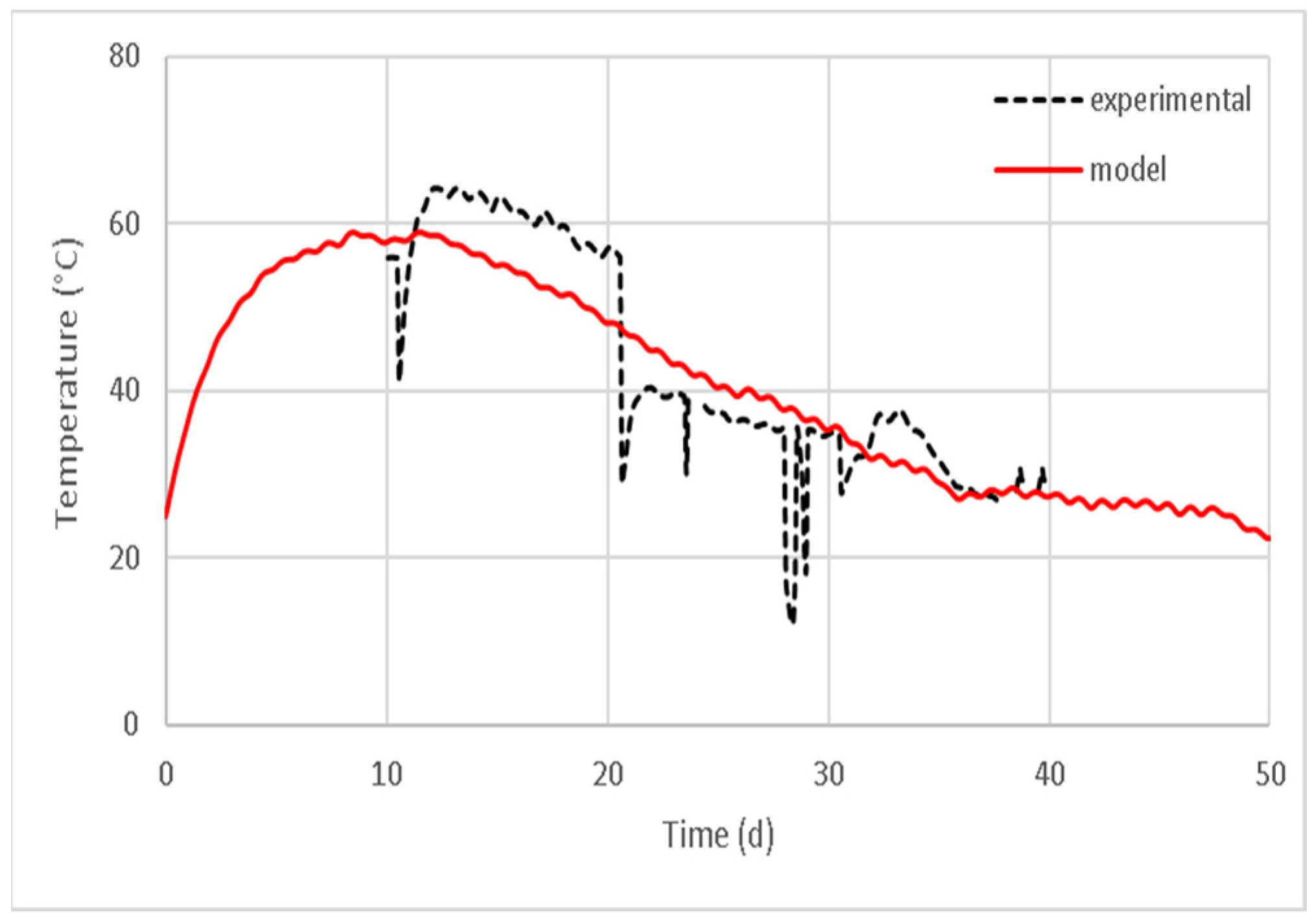
3.2. Comparison between the Modeling and the Experimental Results

3.2.1. Cell Growth

Figure 11 presents the modeled and experimental results for the biomass and temperature in the center of the pile [21]. Starting with the modeled biomass (Equation (23)), it achieved its maximum cell growth in 30–35 days, reaching a value of 0.046 kg/kg dry weight (Table 2), a result that was 4% below that of the biomass obtained experimentally. These results showed that the microbial population reached its stationary phase in 30–35 days. This meant the end of the biodrying stage, and that from day 35 to 50, the pile dried only through the ambient drying in the greenhouse.

Based on the experimental results for the microbial growth and residual substrate (Table 2), a biological yield of 0.3 kg biomass/kg substrate was determined, which meant that from the degradation of the organic matter, only 30% was converted into biomass and that the rest was transformed into CO₂, H₂O, heat and metabolites that alkalized the medium, raising the pH from 5 to 9 [4,33]. Moreover, the net biomass grown was 0.0356 kg biomass/kg dry pile; therefore, there was a substrate consumption of 0.12 kg substrate/kg dry pile, which indicated that the microbial growth consumed approximately 12% of the organic matter. This result is one of the advantages of biodrying, since the organic matter undergoes little degradation, so the dried organic residue would still retain a high calorific value to be used as biofuel [34].

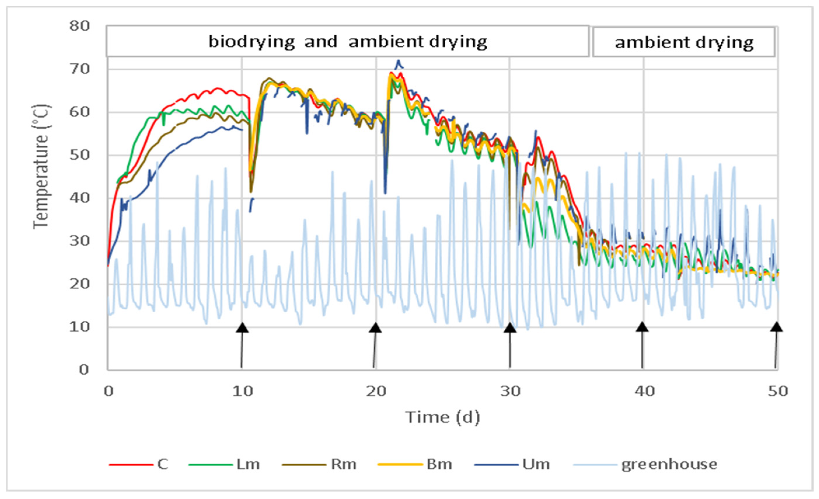
3.2.2. Temperatures at the Center, C, and Midpoints of the pile Lm, Rm, Bm, Um

Period 0 to 10 days. The first phase lasted ten days (Figure 11) and consisted of the rapid growth of the microbial population, which caused the heat generation to exceed its output; therefore, the temperature rose from the initial reading (25 °C). Following this increase, a maximum was reached because the convection heat output balanced the generation: 65 °C in the center, 60 °C in the left and right midpoints and 58 °C in the upper midpoint [21]. It should be noted that [1] reported that the center of the pile was the hottest point, while the surfaces had the lowest temperature.

Figure 11 shows that the profile of the modeled temperature in the center of the pile was very similar to the data obtained experimentally, during the period from 0 to 10 days; the modeled results were, on average 4% below the experimental ones.

Figure 12 and Figure 13 show that the modeled profiles are very similar to those recorded experimentally in the left and right midpoints: 10% below the experimental ones from 0 to 5 days, but identical from 6 to 10 days for the left face, while for the right face they were identical from 0 to 8 days and only 4% higher from 9 to 10 days.

Figure 14 shows the temperature profiles for the base midpoint; however, due to a technical failure, the experimental values were not recorded during the first 10 days, but the modeled profile is very similar to the experimental profile of the center of the pile, because it is a deeper point than the center.

Figure 15 shows the profiles for the upper midpoint: the modeled results were clearly higher by an average of 8% (5 °C difference), and the extremes were more pronounced than the experimental ones, indicating that the model should consider a more accurate calculation for the solar radiation received by this face of the pile.

Period 10 to 20 days. When the first turning was applied (day 10), the experimental temperature in the center dropped rapidly from 65 to 45 °C, due to the heat transfer to the environment (Figure 11); the left and right midpoints cooled from 60 to 42 °C (Figure 12 and Figure 13), there was no record for the base midpoint, and the upper midpoint dropped from 57 to 40 °C (Figure 14 and Figure 15). Then, the temperature rose again rapidly (within a day) to the maximum value, 65–67 °C, for the center and midpoints, due to the microbial activity of a larger population that was oxygenated by turning (a similar behavior was reported by Zambra et al. [5]). The rapid decrease in the temperature during the turning and then the rapid rise, due to the microbial metabolism, could not be modeled, so the modeled results from day 10 to 20 did not consider the pile turning process.

Moreover, the turning also caused moisture loss, and the oxygen supplied was rapidly consumed, so the reduction in moisture started to limit the microbial activity [4]; this limitation caused the microbial growth rate to begin its decline (according to the modeled biomass results in Figure 11), and as a consequence, the heat generation was no longer as intense as at the beginning, and as it was counteracted by the convective heat output, it was observed that the temperature of the center and midpoints slowly decreased from 67 to 60 °C from day 10 to 20.

The modeled and experimental temperature profiles were virtually identical for the center of the pile (Figure 11), while for the left and right midpoints, the modeled results were 13% lower than the experimental ones, due to what was explained above about the turning of the pile, but the model did obtain practically the same cooling rate during this period, as can be seen in the same cooling slope in both the modeled temperature profiles and the experimental results in Figure 12 and Figure 13. The modeled temperature profile for the base midpoint (Figure 14) was 8% lower than the experimental profile but the modeled and experimental cooling slopes are the same. For the upper midpoint of the pile (Figure 15), the modeled results were 10% lower than the experimentally recorded values and with the same cooling slope, between the experimental and modeled values.

Period 20 to 30 days. On the second turning, day 20, exactly the same thing occurred, as was previously described for the first turning: this time the temperature of the center and midpoints (Figure 11, Figure 12, Figure 13, Figure 14 and Figure 15) dropped rapidly from 60 to 50 °C, due to the convection cooling, and the microbial population was oxygenated, thereby increasing the heat generation [4,8] which again caused a rapid rise (in one day) in the temperature, to 70 °C (higher than that reached in the first turning, 65 °C, due to a larger microbial population, although growing at a slower rate, according to the modeled biomass results in Figure 11).

This period, from day 20 to 30, is governed by the decrease in the moisture content, which causes a limitation in the microbial activity, and this limitation increases because the moisture continues to decrease, as a result of the biodrying of the piles (it fell from 60 to 40%, as can be seen in Figure 11). As a result, the heat generation is now less intense, causing the temperature to decrease faster than in the first turning. Thus, the temperature of the center and midpoint layers dropped after the turning, from 70 to 53 °C, during this period (Figure 11, Figure 12, Figure 13, Figure 14 and Figure 15).

From day 20 to 30, the modeled temperature of the center and midpoints of the pile was on average, 25% lower than the experimental temperature. This difference was due to the turning, which was not modeled, as mentioned above, but the modeled results presented in Figure 11, Figure 12, Figure 13, Figure 14 and Figure 15 showed the same cooling slope as the experimental slope, but as a result of the turning (rapid cooling, oxygenation and rapid temperature rise), the experimental temperature values were 25% higher than the modeled values. That is, if no turning had been carried out, the experimental temperature would not have risen to 70 °C and would then have decreased from 55–53 °C to 40–42 °C, as predicted by the model.

It should be noted that the modeled temperature profiles of the center and midpoints of the pile quite accurately represented the temperature extremes of the experimental recorded temperature values, and that these extremes (product of the periods of sunshine and darkness) were more pronounced for the upper midpoint (Figure 15), because it is the one that directly received the solar radiation, with a depth of 16 cm from the upper surface. The temperature extremes were less pronounced for the left and right midpoints because they received the solar radiation obliquely (Figure 12 and Figure 13), they were slightly pronounced for the center because it was twice as deep as the previous ones (Figure 11), and they were very little pronounced for the middle of the soil, because it is the deepest point of the pile, 48 cm (Figure 14).

On the third turning (day 30) the same trend occurred, as previously described, but this time the temperature of the center and midpoints (Figure 11, Figure 12, Figure 13, Figure 14 and Figure 15) dropped rapidly from 54 to 38–35 °C, due to the cooling, and the microbial population oxygenated, increasing the heat generation but to a lesser degree, which caused a less rapid increase in temperature (2 days), rising only to 55 °C (except for points Lm and Bm, where it only rose to 40 and 48 °C, respectively).

The moisture content from day 30 to 35 (which decreased from 40 to 30%, Figure 11) further limited the microbial activity (which was already ending, according to the biomass modeling, Figure 11) of a slightly larger population than on day 20, causing the rate of the heat generation to be the lowest of the entire process and, consequently, the decrease in temperature, in the center and midpoints of the pile, to be more pronounced than in the previous two stages, now from 55 to 32 °C, in only three days; for example, the first temperature decrease was from 67 to 57 °C in 10 days, with a moisture reduction from 68 to 60%, and the second decrease was from 67 to 50 °C, also in 10 days, with a moisture reduction from 60 to 40%.

The modeling of the temperature profile in the center and midpoints (Figure 11, Figure 12, Figure 13, Figure 14 and Figure 15) did not represent these experimental results, due to the turning carried out on day 30, and since this could not be modeled, the modeled results were 35–38% below the experimental ones, and the experimental cooling slope was three times higher than that of the modeled slope; however, the model served as a support to explain all of this behavior.

Period 30 to 50 days. This period was controlled by the environmental conditions inside the greenhouse, because there was no longer a significant metabolic heat generation, since the cell growth had ended, according to the previous modeling performed by Orozco et al. [17]. In this last period, the moisture decreased from 30 to 19%, the values that were insufficient to maintain the water activity (a_w) necessary for the enzymatic reactions of the microorganisms (Figure 11).

From the period 35 to 42 days, the nighttime greenhouse temperature was 15 °C (Figure 9) and the experimental temperature of the center and midpoints tended to decrease from 30 to 28 °C. During the day the greenhouse temperature was 50 °C (Figure 9), so the center and midpoints tended to warm up, but only increased from 28 to 30 °C, because the penetration of the heat by the solar radiation was very slow, due to the low absorptivity of the pile (0.45), resulting from the distance it had to penetrate (16 to 32 cm) during the sunlight period from 8:00 to 19:00 h and because of the low thermal diffusivity of the pile (7.63 × 10⁻⁷ m²/s). From days 35 to 42, the experimental temperature values at the center and the midpoints of the pile and the modeled values were practically the same (Figure 11, Figure 12, Figure 13, Figure 14 and Figure 15).

When the turning was performed (day 42), the experimental temperature at the center and midpoints of the pile dropped to 25 °C and remained practically the same until day 50. The temperature no longer rose after the turning because the microbial activity had already ended, due to a lack of moisture (final pile moisture was 19–20%); at night it dropped to 23 °C and during the day it rose again to 25 °C. Thus, the modeled temperature profiles for the center and base midpoint (Figure 11 and Figure 14, respectively) were 12% higher than the experimental profiles in this same period of 42 to 50 days, because the turning could not be modeled and this was responsible for the cooling, thus causing the modeled profile to be higher than the experimental one.

The modeled profiles for the left and right midpoints of the pile (Figure 12 and Figure 13, respectively).

Again, through the modeling, it was possible to observe that the solar radiation penetrated more strongly at point Um (where it directly received the radiation and was at a depth of 16 cm, Figure 5) and therefore presented the most pronounced temperature extremes; then, they were moderately pronounced for points Lm and Rm (they were at twice the depth of Um) because the radiation struck obliquely; and the least pronounced extremes were those at points C and Bm because the radiation practically no longer penetrated to those pile depths (32 and 48 cm, respectively).

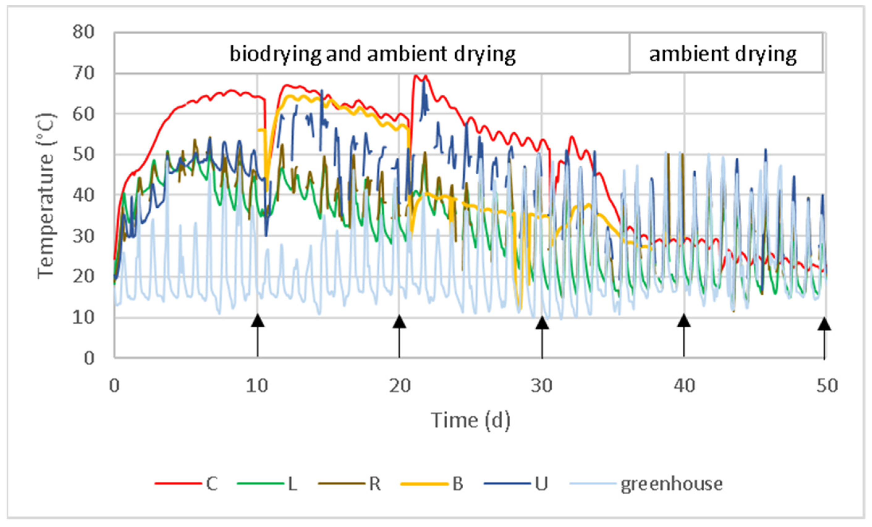
3.2.3. Temperatures on the Surface Faces of the Pile: L, R, B, U

The following paragraphs describe the behavior of the modeled temperature, compared to the experimental results for the points on the surface of the left, right, base and upper faces of the pile (Figure 16, Figure 17, Figure 18 and Figure 19, respectively). The explanations already provided above (the microbial heat generation, moisture, convection and solar radiation) for each of the different biodrying periods are now applied to explain the behavior (experimental and modeled) of the temperature profiles on the surface faces of the pile (L, R, B and U). Thus, these profiles are now discussed, but only globally, so as not to be repetitive, for the period from 0 to 50 days of biodrying.

• Temperature at the base (B) face of the pile

The experimental temperature profile of the base point of the pile in the period 0 to 10 days was not recorded (Figure 18), but the modeled profile shows how it could have been, since as the deepest point (62 cm), it could have presented the same modeled profiles as points Bm and C (due to the depth level), which presented a good agreement with the experimental values.

In the period 10 to 20 days, the modeled temperature values were 15% lower than the experimental values. Then from day 20 to 30, something unexpected occurred because the experimental values of B (40 to 30 °C) were lower than the experimental values (67 to 52 °C) of the base midpoint, Bm (Figure 14), which could be due to an erroneous placement of the temperature sensor after the turning. The experimental values of B were expected to be very similar to those of Bm, since both are located on the same axis, as shown in Figure 5.

For the period 30 to 35 days, the modeled profile was 8% lower than the experimental one for the reasons already given in the corresponding period (low moisture, reduction of microbial heat and natural convection). From day 35 to 50, there was no experimental temperature record, but the model was used, which predicts that the temperature could remain practically at 25 °C.

• Temperatures on the left and right faces of the pile: L and R

The modeled temperature profiles of the left and right surface points of the pile agreed by 95% with the experimental values recorded for days 0 to 7 (Figure 16 and Figure 17). Only for days 7 to 10 did both profiles agree by 85%. On days 10 to 13, both profiles were similar, only in the upper extremes because the turning was carried out on day 10. For the period from day 13 to 20, the modeled and experimental profiles were 90–95% similar. Again, the profiles only agree in the upper extremes (high temperature values during the day) for days 20 to 23, because the turning took place on day 20, and from days 23 to 50, practically both temperature profiles (modeled and experimental) of the left and right surfaces agreed on average by 97%.

It should be noted that the daytime extremes of the modeled and experimental profiles of the left and right surfaces of the pile, during the 0–30 day biodrying period, were lower values (maximum 50 and thereafter dropped to 40 °C for the left surface; for the right surface they dropped from the maximum of 57 to 53 °C) than the experimental values of the center or Bm (65–70 °C to 55 °C), because the sensors were on the surface and therefore the microbial heat was easily dissipated from the pile.

From day 30 to 50, the daytime extremes of both temperature profiles (modeled and experimental) of the right surface were similar to the maximum greenhouse temperature, during the day (48–50 °C), while the values of the left surface only reached 38–40 °C, because this face of the pile was oriented towards the west and therefore the solar radiation fell towards the horizon, and, aside from this, this face was close to the open door of the greenhouse entrance where there was greater convection, hence its lower values.

The same happened at night when the greenhouse temperature was 15–17 °C: the lower extremes (low temperature values during the night), both modeled and experimental, on the left surface, reached minimum values of 16–17 °C, while the values on the right surface were 18–19 °C, due to less convection on this face of the pile (opposite side to the greenhouse entrance).

• Temperature at the upper face of the pile: U

The modeled temperature profile of the upper surface point of the pile agreed by 95% with the experimental values recorded for days 0 to 3 (Figure 19). There was an 80% agreement between the two for days 4 to 10. For days 10 to 13, the two profiles were 97% similar only in the upper extremes, because the turning was conducted on day 10. For the period from day 13 to 20, the modeled and experimental profiles were 90–95% similar. For days 20 to 23, again the profiles only agreed on the upper extremes, because the turning was carried out on day 20; the modeled lower extremes were 22% lower than the experimental values. From day 23 to 50, the modeled and experimental upper surface temperature profiles had, on average a 95% agreement.

The upper extremes of the modeled and experimental profiles of point U during the 13–50 day biodrying period, were values 3–5 °C higher (maximum of 62 °C and from there down to 50 °C), with respect to point R (they fell from the maximum of 57 to 53 °C; Figure 17), because the sensors received the solar radiation directly and the right surface of the pile received it obliquely.

From day 30 to 50, the upper extremes of both temperature profiles (modeled and experimental) of the upper surface in the daytime resembled the maximum greenhouse temperature (48–50 °C), while at night, when the greenhouse temperature was 15–17 °C, the lower extremes, both modeled and experimental, were 18–19 °C, due to less convection on this face of the pile, relative to the large greenhouse space.

Thus, after having addressed in detail the entire biodrying process of the waste pile, a comparative summary of the experimental and modeled results is provided in

Table 5. Percentage difference between the modeled and experimental temperature profiles.

	Time Period (Days)	Center and Midpoints of the Pile					Pile Surfaces or Faces
		Node 1 Center (C)	Node 55 Left Midpoint (Lm)	Node 80 Right Midpoint (Rm)	Node 31 Upper Midpoint (Um)	Node 38 Base Midpoint (Bm)	Node 9 Left (L)	Node 10 Right (R)	Node 3 Upper (U)	Node 4 Base (B)
Biodrying: Microbial activity and Ambient drying	0 to 10	−4	−10	+4	+8	no record	−10	−10	−15	no record
	11 to 20 Turning at 10	0	−13	−13	−10	−8	−7	−7	−7	−15
	21 to 30 Turning at 20	−25	−25	−25	−25	−25	−2	−2	−10	Recoding error
	31 to 35 Turning at 30	−36	−36	−36	−36	−36	−3	−3	−5	−8
Ambient drying	36 to 42 No Turning	0	0	0	0	0	−3	−3	−5	no record
	43 to 50 Turning at 42	+10	+2	+2	0	+10	−3	−3	−5	no record

, which globally and comprehensively shows the primary objective of this work.

The temperature profiles shown by the nine sensors placed in the pile were the result of the balance between the degree of microbial activity and the phenomena of convection, solar radiation and the low thermal diffusivity of the pile.

Thus, during the period of the different levels of the microbial activity (0 to 35 days), it strongly governed the temperature profiles of the center, midpoints and base of the pile, because the heat generated is better “stored”, due to the depth and low thermal diffusivity of the pile; and, these profiles are very little affected by the solar radiation (“high” daytime extremes) and by the convection (“low” nighttime extremes).

While the profiles of the pile surfaces were the product of an “intense” equilibrium, the microbial activity also governed the high temperature values but in conjunction with the solar radiation, but now, the heat generated was easily dissipated by the convection at zero depth, so that during the day there were “high” extremes (but lower than in the center), and at night there were “low” extremes (but of lower value, compared to the center).

During the period of no microbial activity (35 to 50 days), the temperature profiles of the surface faces were governed by the ambient temperature inside the greenhouse: in the daytime, the temperature values tended towards high values (50 °C), mainly due to the solar radiation, and at night the values tended towards low values (15 °C), due to the convection. Temperature profiles of the center, midpoints and base of the pile were only very weakly affected by the ambient temperature variations in the greenhouse, due to the different depth levels of the sensors, 32, 16 and 64 cm, respectively, and the low thermal diffusivity of the pile (7.63 × 10⁻⁷ m²/s): during the day the temperature only rose from 23 to 25 °C, due to the solar radiation, and at night the temperature only dropped from 25 to 23 °C, due to the convection.

3.3. Suggestions for Future Research

In order to improve the model presented in this paper, three different points could be considered:

(a) The microbial growth model requires the incorporation of the effect of moisture in the pile and the effect of pH because the moisture reduction during biodrying stops the growth of the microorganisms when the water activity is less than 0.30. An increase in pH during the biodrying also limits the microbial growth by causing an aqueous environment that is less suitable to the microbial metabolism.

(b) The heat transfer equations need to incorporate the effect of porosity, as it changes along the biodrying process. At the beginning, the porosity is low, but at the end, during the cooling stage of the pile, more free spaces are created, as a result of moisture loss, causing the heat transfer rate to be affected by this variable.

(c) The model requires a drying rate equation to predict the moisture reduction during the biodrying. This equation should consider the effect of the changing porosity and tortuosity of the pile that would affect the effective diffusivity of the evaporated water. Furthermore, it should be kept in mind that the condensation level of the evaporated water is a phenomenon that occurs during the turning of the pile caused by sudden cooling. Finally, the equation also should take into account the effect of the high temperatures of the pile during the thermophilic stage on the drying rate.

4. Conclusions

For the biodrying start-up and maximum microbial activity period (0 to 10 days), the modeled temperature profiles of the center, midpoints and base of the pile showed a high correspondence with the experimental profiles, with a difference of just 4 to 8%, while this correspondence was good for the modeled profiles of the surface faces of the pile with a difference of 10 to 15%.

For the period of maximum microbial activity and its subsequent decline until the cessation of its activity (10 to 35 days), the modeled profiles of the center, midpoints and base of the pile presented a low correspondence with the experimental profiles, with the largest difference of 10 to 36% attributed to the pile turning on days 10, 20 and 30. The turning process could not be modeled, so the modeled temperature profile values were 20 to 30% lower than the experimental ones. However, the temperature reduction slope, obtained for the nine modeled profiles, was identical to the experimental cooling slope of the corresponding monitoring points (except for the period from day 30 to 35 ), showing that the modeling was adequate for this pile biodrying period, despite the large difference between the modeled and experimental values.

During days 2 to 35, when the thermophilic stage of the biodrying was taking place, the most significant changes in the temperature occurred, due to microbial development, ranging between 40 and 64 °C in the center of the pile. The highest rates of water removal occurred causing a significant decrease in moisture (from 75 to 32%) in the center of the pile. The growth of the microbial population completely ceased on day 35 when the moisture of the pile reached values of 33–31%, probably due to the fact that the water activity of the solid waste was already insufficient to maintain the cellular metabolic activity.

For the period when the microbial activity had completely ceased (from day 35 to 50), there was a high correspondence between the nine modeled temperature profiles and the experimental ones with a difference of only 3 to 5%, showing an adequate modeling of the solar radiation and convection phenomena, together with the different depth levels of the sensors and the low thermal diffusivity of the pile waste. In this cooling stage, the microbial growth was null, causing the temperature in the center of the pile to drop from 40 to 23–25 °C, and the drying rate (only solar radiation and convection) was low, causing the humidity to drop slowly from 32 to 18%

Finally, the finite differences the modeling allows to deal with the convection and solar radiation for each face of the pile, separately, so that each surface can have the same or different convective index, and in the case of radiation, it falls on each face of the pile differently due to the “changing” position of the sun during the day.

References

1. Rada, E.C.; Franzinelli, A.; Taiss, M.; Ragazzi, M.; Panaitescu, V.; Apostol, T. Lower heating value dynamics during municipal solid waste bio-drying. Environ. Technol. 2007, 28, 463–469. [Google Scholar] [CrossRef] [PubMed]
2. Ma, J.; Zhang, L.; Mu, L.; Zhu, K.; Li, A. Thermally assisted bio-drying of food waste: Synergistic enhancement and energetic evaluation. Waste Manag. 2018, 80, 327–338. [Google Scholar] [CrossRef] [PubMed]
3. Xin, L.; Li, X.; Bi, F.; Yan, X.; Wang, H.; Wu, W. Accelerating food waste composting course with biodrying and maturity process: A pilot study. ACS Sustain. Chem. Eng. 2021, 9, 224–235. [Google Scholar] [CrossRef]
4. Contreras-Cisneros, R.M.; Orozco-Álvarez, C.; Piña-Guzmán, A.B.; Ballesteros-Vásquez, L.C.; Molina-Escobar, L.; Alcántara-García, S.S.; Robles-Martínez, F. The relationship of moisture and temperature to the concentration of O2 and CO2 during biodrying in semi-static piles. Processes 2021, 9, 520. [Google Scholar] [CrossRef]
5. Zambra, C.; Rosales, C.; Moraga, N.; Ragazzi, M. Self-heating in bioreactor: Coupling of heat and mass transfer with turbulent convection. Int. J. Heat. Mass. Transfer. 2011, 54, 5077–5086. [Google Scholar] [CrossRef]
6. Zambra, C.; Moraga, N.; Escudey, M. Heat and mass transfer in unsaturated porous media: Moisture effects in compost pile self-heating. Int. J. Heat. Mass. Transfer. 2011, 54, 2801–2810. [Google Scholar] [CrossRef]
7. Zambra, C.E.; Moraga, N.O.; Rosales, C.; Lictevout, E. Unsteady 3D heat and mass transfer diffusion coupled with turbulent forced convection for compost piles with chemical and biological reactions. Int. J. Heat. Mass. Transfer. 2012, 55, 6695–6704. [Google Scholar] [CrossRef]
8. Zhang, Y.; Lashermes, G.; Houot, S.; Doublet, J.; Steyer, J.; Zhu, Y.; Barriuso, E.; Garnier, P. Modelling of organic matter dynamics during the composting process. Waste Manag. 2012, 32, 19–30. [Google Scholar] [CrossRef] [PubMed]
9. Mason, I.; Milke, M. Physical modelling of the composting environment: A review. Part 1: Reactor systems. Waste Manag. 2005, 25, 481–500. [Google Scholar] [CrossRef] [PubMed]
10. Mason, I. Mathematical modelling of the composting process: A review. Waste Manag. 2006, 26, 3–21. [Google Scholar] [CrossRef] [PubMed]
11. Vlyssides, A.; Mai, S.; Barampouti, E. An integrated mathematical model for composting of agricultural solid wastes and industrial wastewater. Bioresour. Technol. 2009, 100, 4797–4806. [Google Scholar] [CrossRef] [PubMed]
12. Guardia, A.; Petiot, C.; Benoist, J.; Druilhe, C. Characterization and Modeling of the Heat Transfers in a Pilot-Scale Reactor During Composting Under Forced Aeration. Waste Manag. 2012, 32, 1091–1105. [Google Scholar] [CrossRef] [PubMed]
13. Petric, I.; Selimbasic, V. Development and validation of mathematical model for aerobic composting process. Chem. Eng. J. 2008, 139, 304–317. [Google Scholar] [CrossRef]
14. Díaz-Megchún, J. Análisis del Proceso Térmico Durante el Biosecado de Residuos Sólidos Orgánicos. Master Thesis, Instituto Politécnico Nacional, Mexico City, México, 2014. [Google Scholar]
15. Lawrance, A.; Haridas, A.; Savithri, S.; Arunagiri, A. Development of mathematical model and experimental validation for batch bio-drying of municipal solid waste: Mass balances. Chemosphere 2022, 287, 132272. [Google Scholar] [CrossRef] [PubMed]
16. Lawrance, A.; Santhoshi-Gollapalli, M.V.; Savithri, S.; Haridas, A.; Arunagiri, A. Modelling and simulation of food waste bio-drying. Chemosphere 2022, 294, 133711. [Google Scholar] [CrossRef] [PubMed]
17. Orozco-Álvarez, C.; Molina-Carbajal, E.; Díaz-Megchún, J.; Osorio-Mirón, A.; Robles-Martínez, F. Desarrollo de un modelo matemático para el biosecado de residuos sólidos orgánicos en pilas. Rev. Int. Contam. Ambient. 2019, 35, 79–90. [Google Scholar] [CrossRef]
18. Brebbia, C. The Boundary Element Method for Engineers, 1st ed.; Halsted Press: New York, NY, USA, 1978. [Google Scholar]
19. Zienkiewicz, O.C.; Taylor, R.L.; Zhu, J.Z. The Finite Element Method: Its Basis and Fundamentals, 6th ed.; Elsevier: Oxford, UK, 2005; Chapter 5; pp. 138–178. [Google Scholar]
20. Leveque-Randall, J. Finite Difference Methods for Differential Equations. In Draft Version for Use in the Course AMath; University of Washington: Seattle, WA, USA, 2005; Chapters 1 and 2; pp. 585–586. [Google Scholar]
21. Orozco Alvarez, C.; Díaz-Megchún, J.; Macías-Hernández, M.J.; Robles-Martínez, F. Efecto de la frecuencia de volteo en el biosecado de residuos sólidos orgánicos. Rev. Int. Contam. Ambient. 2019, 35, 979–989. [Google Scholar] [CrossRef]
22. Cerna, E.M.; Stanciu, D. Thermal Coupling Numerical Models for Boundary Layer Flows over a Finite Thickness Plate Exposed to a Time-Dependent Temperature. In Series on Mathematical Modelling of Environmental and Life Sciences Problems, Proceedings of the Fourth Workshop, Constanta, Romania, September 2005; Ion, S., Marinoschi, G., Popa, C., Eds.; Editura Academiei Române: Bucharest, Romania, 2005; pp. 55–68. [Google Scholar]
23. Beers, K.J. Numerical Methods for Chemical Engineering; Cambridge University Press: New York, NY, USA, 2007; Chapter 2. [Google Scholar]
24. Forsythe, G.; Wasow, W. Finite Difference Methods for Partial Differential Equations; John Wiley & Sons: Hoboken, NJ, USA, 1960. [Google Scholar]
25. Zwillinger, D. Handbook of Diferential Equations; Academic Press: Cambridge, MA, USA, 1996; Chapter 6. [Google Scholar]
26. Minkowycz, J.; Sparrow, E.; Schneider, G.; Pletcher, R. Handbook of Numerical Heat Transfer; John Wiley & Sons: Hoboken, NJ, USA, 1988. [Google Scholar]
27. Lapidus, L.; Pinder, G.F. Numerical Solution of Partial Differential Equations in Science and Engineering; John Wiley & Sons: Hoboken, NJ, USA, 1999; Chapter 2. [Google Scholar]
28. Cengel, Y.; Ghajar, A. Transferencia de Calor y Masa, 3rd ed.; McGraw-Hill: México City, México, 2011; Chapter 5. [Google Scholar]
29. Myers, G. Analytical Methods in Conduction Heat Transfer; McGraw-Hill: New York, NY, USA, 1971. [Google Scholar]
30. Bailey, J.E.; Ollis, D.F. Metabolic Stoichiometry and Energetics. In Biochemical Engineering Fundamentals; McGraw-Hill: Dunfermline, UK, 1986; pp. 228–306. [Google Scholar]
31. Moraga, N.; Corvalán, F.; Escudey, M.; Arias, A.; Zambra, C. Unsteady 2D coupled heat and mass transfer in porous media with biological and chemical heat generation. Int. J. Heat. Mass. Transfer. 2009, 52, 5841–5848. [Google Scholar] [CrossRef]
32. ASHRAE. Manual de Radiación Solar; McGraw Hill: New York, NY, USA, 2015. [Google Scholar]
33. Oviedo-Ocaña, E.R.; Marmolejo-Rebellón, L.F.; Torres-Lozada, P. Influencia de la frecuencia de volteo para el control de la humedad de los sustratos en el compostaje de biorresiduos de origen municipal. Rev. Int. Contam. Ambient. 2014, 30, 91–100. [Google Scholar]
34. Robles Martínez, F.; Gerardo Nieto, O.; Piña Guzmán, A.B.; Montiel Frausto, L.; Colomer Mendoza, F.; Orozco Álvarez, C. Obtención de un combustible alterno a partir del biosecado de residuos hortofrutícolas. Rev. Int. Contam. Ambient. 2013, 29, 79–88. [Google Scholar]
Figure 1. Temperature profile of the center (C) and inner layers (Lm, Rm, Bm, Um) of the pile during biodrying. (↑) turning point (Modified after [21]).
Sustainability 14 14705 g001
Figure 2. Temperature profile of the center (C) and lateral faces (L, R, B, U) of the pile during biodrying. (↑) turning point (Modified after [21]).
Sustainability 14 14705 g002
Figure 3. Distribution of the 27 nodes in the rectangular prism.
Sustainability 14 14705 g003
Figure 4. Examples of the volume elements with their nodes and the “cut” at the boundary of the rectangular prism (where Ax = ∆x, Ay = ∆y and Az = ∆z).
Sustainability 14 14705 g004
Figure 5. Correspondence of the thermocouples in the pile with the nodes of the model to be developed. 1: center (C); 3: upper (U); 4: base (B); 31: upper midpoint (Um); 38: base midpoint (Bm); 9: left (L); 10: right (R); 55: left midpoint (Lm); 80: right midpoint (Rm); there were no thermocouples at nodes 0, 2, 34 and 35. Greenhouse temperature: Tα. Convection and solar radiation, h and q, respectively, on the different faces or surfaces of the pile: north, south, east and west; where Ax = ∆x, Ay = ∆y and Az = ∆z.
Sustainability 14 14705 g005
Figure 6. Volume element (in red) of node 1 and the nodes to which it is linked in the three directions.
Sustainability 14 14705 g006
Figure 7. Volume element of nodes 9 and 10 and the nodes to which they are linked in the three directions.
Sustainability 14 14705 g007
Figure 8. Volume element of nodes 3 and 4 and the nodes to which they link in all three directions; cut at ∆y.
Sustainability 14 14705 g008
Figure 9. Temperature record inside the greenhouse ( T α i ) during the biodrying [14].
Sustainability 14 14705 g009
Figure 10. Record of the direct solar radiation inside the greenhouse during the biodrying [14].
Sustainability 14 14705 g010
Figure 11. Experimental [14] and modeled results during the waste pile biodrying.
Sustainability 14 14705 g011
Figure 12. Temperature profile at the left midpoint of the pile: sensor Lm = node 55.
Sustainability 14 14705 g012
Figure 13. Temperature profile at the right midpoint of the pile: sensor Rm = node 80.
Sustainability 14 14705 g013
Figure 14. Temperature profile at the base midpoint of the pile: sensor Bm = node 38.
Sustainability 14 14705 g014
Figure 15. Temperature profile at the upper midpoint of the pile: sensor Um = node 31.
Sustainability 14 14705 g015
Figure 16. Temperature profile of the surface point of the left face of the pile: sensor L = node 9.
Sustainability 14 14705 g016
Figure 17. Temperature profile of the surface point of the right face of the pile: sensor R = node 10.
Sustainability 14 14705 g017
Figure 18. Temperature profile of the surface point of the base face of the pile: sensor B = node 4.
Sustainability 14 14705 g018
Figure 19. Temperature profile of the surface point of the upper face of the pile: sensor U = node 3.
Sustainability 14 14705 g019