Techno-Economic-Environmental Energy Management of a Micro-Grid: A Mixed-Integer Linear Programming Approach

Abstract

In recent years, owing to the effect of fossil fuels on global warming, the exhaustion of oil fields, and the lucrative impacts of renewable energy resources (RESs), the penetration of RESs has been increasing significantly in power systems. An effective way to benefit from all RESs advantages is by applying them in microgrid systems (MGS). Furthermore, MGS can ease the way for utilizing a large amount of RESs, if its economic-environmental-technical aspects of it are taken into account. In this regard, this paper proposes an optimal solution for the energy management of a microgrid by considering a comprehensive study. In the proposed methodology, different distributed energy resources such as wind turbines generator (WTG), energy storage (ES), combined heat and power (CHP), rubbish burning agent (RBA), and diesel generators (DG) are modeled. In addition, electric vehicles (EVs) are considered a load with uncertainty. The objective function of the proposed method is to minimize the microgrid’s total cost by considering the microgrid’s emission cost and technical constraints. In this study, the microgrid’s technical, environmental, and economic aspects are investigated. In addition, the optimization problem is converted into a mixed-integer linear programming method by using the proper linearization method. In this paper, the increasing effect of wind energy penetration rate on the total price also has been studied. The simulation results show that by increasing the wind energy penetration rate by up to 30% of total power, the total cost will decrease by up to 30.9%.

1. Introduction

Due to the increasing electrical energy consumption worldwide, it is necessary to expand electrical energy production centers. There are two main approaches to generating electrical power: The first approach is to produce electrical energy at limited points such as a central network and transfer it throughout the network. Most of such power plants use fossil fuels for energy conversion. The second approach is to use renewable energy. The main problem of fossil fuel power plants is environmental pollution and the emission of greenhouse gases, which causes global warming; furthermore, centralized transmission by large power plants increases loss [1]. Renewable energies such as wind and solar energy significantly mitigate environmental issues. However, due to the intermittent and fluctuating nature of renewable sources, the stability and security of the system are affected [2]. One of the practical ways to make better use of renewable energy sources is microgrid technology. The microgrid can be used in grid-connected or island mode. Energy management will help islanded microgrids achieve sustainability. In addition, when the microgrid connects to the network, it provides exchanging possibility with the distribution network. One of the challenges facing microgrid energy management systems (MG-EMS) is finding an optimal schedule to use the available resources. In the literature, two methods have been implemented for EM in MGs. The first method includes the use of meta-heuristic methods, and the second method is based on mathematical programming (MP) methods such as mixed integer linear programing (MILP) and mixed integer non-linear programing (MINLP) [3]. In meta-heuristic methods (such as QTLBO in [4] and GA in [5]), there is no guarantee of reaching the global point, and it is possible to stock in local optimal points. In addition, different results may be obtained based on the initial conditions and various iterations. In methods based on MP, it is possible to reach the global optimal point. To find the global optimal point in a non-linear system, the model must be converted to linear by approximation. Then the optimal point is obtained from linear optimization methods (such as [6]). Of course, it is possible to obtain the optimal point in non-linear systems using MP methods, and many non-linear techniques have been presented in the literature from the classic genetics algorithms to its novel Mendelian variants [7]. Recently, heuristic nature-inspired nonlinear techniques have been successfully used in a wide range of applications from AI model design [8] to self-organized control [9]. However, there is no guarantee that the optimal point will be global (such as MINLP in [10]). In [11], an EMS issue with MATLAB’s Fmincon function has been studied; due to the nonlinearity of the fuel consumption cost, there is no possibility of reaching the global point. In [12], the focus is on reducing the degradation cost of energy storage. In addition, to make better decisions based on the predicted data, the CCP method has been used. Ref [13] reports a practical approach for optimal management of a MEMG performance by considering the uncertainties associated with demand prediction. In this article, the connection with an upstream network is considered; however, the supposed model for linearization is not accurate. Ref [14] has been regarded as a multi-objective optimal scheduling model that includes operational economy and satisfaction of electricity consumption on the demand side. The sparrow search algorithm is used to solve the MINLP problem. In [15], the impact of EVs in isolated hybrid microgrids with WT, PV, ES, and DG has been studied. In this article, there is no connection with the upstream network, and the constraints related to the network elements are very few, which makes the optimization far from reality. Ref [15] has used a virtual power plant (VPP), considering a pumped storage plant (PSP) and electrical vehicles (EVs) as energy storage. The presence of EVs in the network has been considered through a parking lot, but the variety and numbers of energy production sources in this article are few. Ref [16] provides an optimal energy consumption for apartments; in this article, there is a possibility of energy exchange between apartments. However, this study has not considered renewable energy sources, and in addition, the microgrid’s uncertainties are not discussed. Ref [17] examines the efficient power exchange by Cuckoo Search Algorithm (CSA). This paper proves that CSA enables flexible and compatible electricity exchange between microgrids and the commercial grid. Nevertheless, CHP, EVs, and uncertainties related to the network are not considered, and there is no connection with the upstream network. Ref [18] surveys the methods of microgrid element selection, such as a diesel generator and energy storage, using a hybrid optimization model for electric renewables (HOMER) software. This article investigated the network in island mode and only used solar cells as a source of renewable energy production. The type of cost function, methodology, and type of energy production resources considered for each article are shown in

Table 1. Comparison of EMS in the literature review.

Ref	DG	CHP	WT	EV	ES	Methodology	Objective Function
[11]	✓	✗	✓	✗	✓	Fmincon	Multi-Objective
[6]	✓	✗	✓	✓	✓	MILP	Minimizing distribution grid losses
[4]	✓	✗	✓	✗	✓	QTLBO	Optimizing energy flow in microgrids
[1]	✗	✗	✓	✗	✓	ABC	Minimizing cost
[13]	✗	✓	✓	✗	✓	MILP	Minimizing cost
[17]	✓	✗	✓	✓	✓	MILP	Maximizing profit
[14]	✗	✓	✓	✗	✓	MILP	Multi-Objective
[12]	✓	✗	✓	✗	✓	CCP	Minimizing cost
[18]	✓	✗	✓	✗	✓	MILP	Minimizing cost
[19]	✓	✗	✗	✗	✓	MILP	Minimizing cost
[20]	✓	✗	✓	✗	✓	DNN/RL	Maximizing profit
[21]	✗	✗	✗	✓	✓	LSTM-DL	Multi-Objective
[22]	✗	✗	✓	✗	✓	Cooperative game	Multi-Objective
This paper	✓	✓	✓	✓	✓	MILP	Minimizing total cost

.

Most of the studies have focused on minimizing the cost of energy production and have not paid attention to the resource constraints and complexities of the microgrid. In addition, several articles have considered the simultaneous investigation of environmental effects and uncertainties related to load, weather conditions, and the presence of electric vehicles. In addition, reaching the global optimal point requires linearization of the system, and some articles use non-linear models to achieve the optimal point. Therefore, the main contributions of this work are summarized as follows:

• Due to the nonlinearity of the relationships governing the elements of energy production in the microgrid (such as the diesel generator fuel relationship), it is impossible to achieve the global optimal point with non-linear methods. The best solution is to use an exact linear model to reach the global optimal point. Therefore, an accurate linear model based on the piecewise linear approximation method for microgrid energy management is presented in this paper.
• In order to have closer simulation results to reality, all network costs and limitations should be considered, which have been given less attention in recent studies. Therefore, in this article, the costs related to the emission, the cost of battery degradation, the cost of providing thermal load, the connection with the upstream network, the restrictions associated with the presence of electric vehicles, interruptible load, etc., are considered.
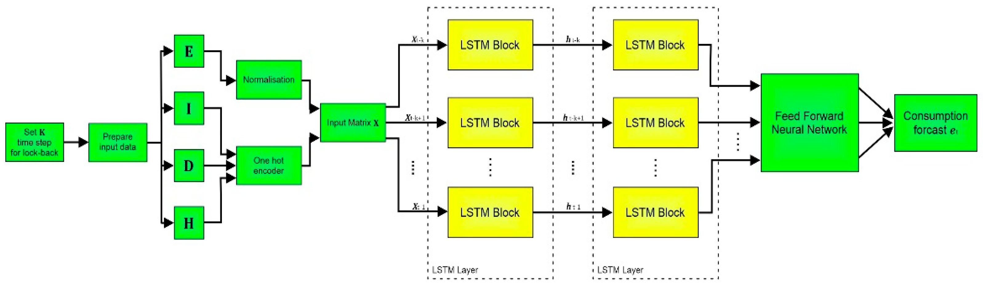
• With the increasing penetration of RESs and the crucial role of stochastic parameters such as load demand, and electricity price in the energy management of MGs, the accuracy of forecasting these parameters has a decisive impact on the total cost of MGs. In this regard, a method based on deep long-short term memory (LSTM) networks is utilized to model these parameters.

The rest of this paper is organized as follows: the mathematical model is presented in Section 2. Section 3 shows the simulation result and sensitivity analysis. Finally, the conclusion is provided in Section 4.

2. Mathematical Model

In this paper, the objective of EMS is to minimize the day ahead energy cost. The cost function of the system is shown in Equation (1).

$$\begin{gathered} Cost Function=\underset{\left(1\right)}{\underbrace{{\displaystyle \sum }_t(T{C}_t^{buy}+T{C}_t^{IL})}}+\underset{\left(2\right)}{\underbrace{{\displaystyle \sum }_t({\displaystyle \sum }_{h}T{C}_{h,t}^{CHP}+{\displaystyle \sum }_{r}T{C}_{h,t}^{RBA}}}) \\ \hspace{1em}\hspace{1em}\hspace{1em}+\underset{\left(3\right)}{\underbrace{{\displaystyle \sum }_t{\displaystyle \sum }_{d}T{C}_{d,t}^{DG}}}+\underset{\left(4\right)}{\underbrace{{\displaystyle \sum }_t({\displaystyle \sum }_{w}T{C}_{w,t}^W{\displaystyle \sum }_{e}T{C}_{e,t}^{Batt})}} \end{gathered}$$

(1)

The first part of Equation (1) represents the change of cost and interruptible load. The amount $T{C}_t^{buy}$ can be positive or negative depending on the amount of buying or selling from the network. $T{C}_t^{IL}$ indicates the amount of cost paid by the consumer; in the form of a contract, it is paid for by disconnecting the load at certain hours. The second part shows the cost of Combined Heat and Power (CHP) and Rubbish Burning Agent (RBA). The third part shows the cost of diesel generators, and the fourth part shows the costs of wind turbine maintenance and degradation cost of energy storage.

2.1. Upstream Network

Connection with the global electricity grid allows excess electrical energy to be sold. In addition, when renewable energy production is low, or consumption is high, the grid will purchase the required energy. Equation (2) shows the cost paid or received from the network for the exchange power, and Equation (3) shows the minimum and maximum of exchanged power [13].

$$T{C}_t^{buy}=P_t^{buy}\times C_t^{buy}\times \Delta t$$

(2)

$$P_{min}^{buy}\le P_t^{buy}\le P_{max}^{buy}$$

(3)

2.2. Interruptible Load

Interruptible Load (IL) is an optional contract for consumption reduction between the consumer and the producer to provide power during peak hours. The total cost of the interruptible load is shown in Equations (4) and (5) [22].

$$T{C}_t^{IL}=a^{RBA}\times P_t^{IL}$$

(4)

$$0\le P_t^{IL}\le P_t^{Inflex}$$

(5)

2.3. Combined Heat and Power

In the proposed structure, the CHP is responsible for supplying the thermal load and part of the electrical power; the heat exchanger is considered a gas turbine that converts the chemical energy of natural gas into electricity by using a generator. The calorific value released by fuel combustion can be used to provide thermal load. The boiler is also used as an auxiliary power source to supply excess thermal energy. Moreover, to increase system flexibility, thermal storage is considered. Equations (6)–(8) represent fuel, emission, and total cost of CHP. Moreover, Equations (9)–(12) indicate the constraints related to thermal power provision and Equations (14)–(17) show the admissible range for the heat variables [17].

$$T{C}_{h,t}^{CHP}=F{C}_{h,t}^{CHP}+E{C}_{h,t}^{CHP}$$

(6)

$$F{C}_{h,t}^{CHP}=(f_{h,t}^{Boiler}+f_{h,t}^{CHP}){\rho }_{ }^{NG}$$

(7)

$$E{C}_{h,t}^{CHP}={\displaystyle \sum }_p{\mathrm{Ex}}_{p,\mathrm{h}}\times { \mathrm{EF}}_{p,\mathrm{h}}\times (f_{h,t}^{Boiler}+f_{h,t}^{CHP})$$

(8)

$$H_{h,t}^{Boiler}=f_{h,t}^{Boiler}{\eta }_h^{Boiler}$$

(9)

$$H_{h,t}^{CHP}=\frac{f_{h,t}^{CHP}{\alpha }_h^{CHP}}{1+{\alpha }_h^{CHP}}$$

(10)

$$P_{h,t}^{CHP}=\frac{f_{h,t}^{CHP}}{1+{\alpha }_h^{CHP}}$$

(11)

$$H_t^D={\displaystyle \sum }_h{H}_{h,t}^{Boiler}+H_{h,t}^{CHP}+H_{h,t}^f$$

(12)

$$H_{h,t}^s-H_{h,t}^f=H_{h,t+1}^s$$

(13)

$$H_{h,t}^s\le H_h^{\mathrm{S},\mathrm{MAX}}$$

(14)

$$H_{h,0}^s=H_{h,24}^s$$

(15)

$$f_{h,t}^{Boiler}\le f_h^{Boiler,\mathrm{MAX}}$$

(16)

$$f_{h,t}^{CHP}\le f_h^{CHP,\mathrm{MAX}}$$

(17)

2.4. Rubbish Burning Agent

RBA is an electrical power generation unit based on burning urban solid waste. Equations (18)–(20) demonstrate the fuel, emission, and total cost of RBA, and Equation (21) defines the value of generated power by RBA [13].

$$T{C}_{r,t}^{RBA}=F{C}_{r,t}^{RBA}+E{C}_{r,t}^{RBA}$$

(18)

$$F{C}_{r,t}^{RBA}=P_{r,t}^{RBA}\times {\rho }^{RBA}\times \Delta t$$

(19)

$$E{C}_{r,t}^{RBA}={\displaystyle \sum }_p{\mathrm{Ex}}_{\mathrm{p},\mathrm{r}}\times { \mathrm{EF}}_{\mathrm{p},\mathrm{r}}\times \left(P_{r,t}^{RBA}\right)$$

(20)

$$P_{r,t}^{RBA}=\frac{{\propto }_{\mathrm{T}}^{\mathrm{RBA}}h{v}^{RBA}{f}_{r,t}^{RBA}}{\Delta t}$$

(21)

2.5. Diesel Generator

Diesel generators are typically used when batteries are discharged, and renewable resources are not available. In other words, diesel generators can be used in emergencies to compensate the energy shortage due to their durability, low initial cost, and quick start-up. The start-up, fuel, and maintenance costs could be considered in the diesel generator model. Equation (22) indicates the total cost of diesel generator usage, which consists of three parts: fuel, start-up, and emission costs, shown in Equations (23)–(25). The constraints of ramp-up and ramp-down rates are represented in Equations (27) and (28). In addition, Equations (29)–(33) show the constraints of diesel generator up and down minimum time. In addition, the relationships in [23] have been used to linearize the fuel consumption cost.

$$T{C}_{d,t}^{DG}=F{C}_{d,t}^{DG}+S{C}_{d,t}^{DG}+E{C}_{d,t}^{DG}$$

(22)

$$F{C}_{d,t}^{DG}=(a_d^{DG}{(P_{d,t}^{DG})}^2+b_d^{DG}{(P_{d,t}^{DG})}^{ }+c_d^{DG})u_{d,t}$$

(23)

$$S{C}_{d,t}^{DG}=SU{C}_d(u_{d,t}-u_{d,t}^{\prime })$$

(24)

$$E{C}_{d,t}^{DG}={\displaystyle \sum }_p({\mathrm{Ex}}_{\mathrm{p},\mathrm{d}}\times { \mathrm{EF}}_{\mathrm{p},\mathrm{d}})\times P_{d,t}^{DG}$$

(25)

$$P_d^{DG,MIN} u_{d,t}\le P_{d,t}^{DG}\le P_d^{DG,MAX} u_{d,t}$$

(26)

$$P_{d,t}^{DG}-P_{d,t-1}^{DG}\le (u_{d,t}-u_{d,t}^{\prime })P_d^{DG,MIN}+(1-u_{d,t}+u_{d,t}^{\prime })RU{R}_d$$

(27)

$$P_{d,t-1}^{DG}-P_{d,t}^{DG}\le (u_{d,t-1}-u_{d,t-1}^{\prime })P_d^{DG,MIN}+(1-u_{d,t-1}+u_{d,t-1}^{\prime })RD{R}_d$$

(28)

$${\mathrm{N}}_{\mathrm{d},\mathrm{t}-1}^{\mathrm{DG},\mathrm{on}}+{\mathrm{u}}_{\mathrm{d},\mathrm{t}}-(1-{\mathrm{u}}_{\mathrm{d},\mathrm{t}})\mathrm{M}\le {\mathrm{N}}_{\mathrm{d},\mathrm{t}}^{\mathrm{DG},\mathrm{on}}\le {\mathrm{N}}_{\mathrm{d},\mathrm{t}-1}^{\mathrm{DG},\mathrm{on}}+{\mathrm{u}}_{\mathrm{d},\mathrm{t}}$$

(29)

$${\mathrm{N}}_{\mathrm{d},\mathrm{t}}^{\mathrm{DG},\mathrm{on}}\le {\mathrm{u}}_{\mathrm{d},\mathrm{t}} \mathrm{M}$$

(30)

$$N_{d,t-1}^{DG,on}\ge T_d^{DG,on}\left(u_{d,t-1}-u_{d,t}\right)$$

(31)

$${\mathrm{N}}_{\mathrm{d},\mathrm{t}-1}^{\mathrm{DG},\mathrm{off}}+1-{\mathrm{u}}_{\mathrm{d},\mathrm{t}}-{\mathrm{u}}_{\mathrm{d},\mathrm{t}} \mathrm{M}\le {\mathrm{N}}_{\mathrm{d},\mathrm{t}}^{\mathrm{DG},\mathrm{off}}\le {\mathrm{N}}_{\mathrm{d},\mathrm{t}-1}^{\mathrm{DG},\mathrm{off}}+1-{\mathrm{u}}_{\mathrm{d},\mathrm{t}}$$

(32)

$${\mathrm{N}}_{\mathrm{d},\mathrm{t}}^{\mathrm{DG},\mathrm{off}}\le (1-{\mathrm{u}}_{\mathrm{d},\mathrm{t}})\mathrm{M}$$

(33)

2.6. Wind Turbine

A wind turbine is used to convert kinetic energy to electrical energy. Therefore, it is considered a source of electrical energy production. The gearbox is an essential part of most wind turbines. The gears convert slow rotation of rotor blades into high-speed shaft rotation, and electrical power is produced. Equation (34) defines the cost of wind turbine maintenance. Equation (35) is the wind turbine’s amount of power, depending on the wind speed.

$$T{C}_{w,t}^W=(O\&M_w)\times P_{w,t}^W$$

(34)

$$P_{w,t}^W=\left\{\begin{array}{c}{\mathrm{Pw}}_{\mathrm{w}}^{\max } { \mathrm{v}}_{\mathrm{w}}^{\mathrm{R}}<{\mathrm{v}}_{\mathrm{t}}<{ \mathrm{v}}_{\mathrm{w}}^{\mathrm{COUT}}\\ \frac{{\mathrm{Pw}}_{\mathrm{w}}^{\max }\left({\mathrm{v}}_{\mathrm{t}}-{ \mathrm{v}}_{\mathrm{w}}^{\mathrm{CIN}}\right)}{{ \mathrm{v}}_{\mathrm{w}}^{\mathrm{R}}-{ \mathrm{v}}_{\mathrm{w}}^{\mathrm{CIN}}} { \mathrm{v}}_{\mathrm{w}}^{\mathrm{CIN}}<{\mathrm{v}}_{\mathrm{t}}<{\mathrm{v}}_{\mathrm{w}}^{\mathrm{R}}\\ 0 {\mathrm{v}}_{\mathrm{t}}<{ \mathrm{v}}_{\mathrm{w}}^{\mathrm{CIN}}, {\mathrm{v}}_{\mathrm{t}}>{ \mathrm{v}}_{\mathrm{w}}^{\mathrm{COUT}}\end{array}\right.$$

(35)

2.7. Energy Storage

In a MG, a battery is used for energy storage due to the unpredictability and intermittent nature of renewable energy sources. In this condition, the battery acts as a backup during off-peak hours and reduces cost during peak hours. The energy storage can be charged or discharged at any time. In modeling a battery, minimum and maximum power, charge, and discharge level can be considered. The ES replacement and degradation costs are shown in Equation (36); constraints of charge and discharge levels are defined in Equations (37)–(39). The ES’s State Of Charge (SOC) is indicated in Equation (41) per hour, and Equation (42) shows the acceptable range of SOC [22].

$$T{C}_{e,t}^{ }=a_e^{ES}\left(P_{e,t}^{CH}+P_{e,t}^{DCH}\right)+b_e^{ES}$$

(36)

$$P_{e,t}^{State}=P_{e,t}^{DCH}-P_{e,t}^{CH}$$

(37)

$$0\le P_{e,t}^{CH}\le P_e^{MAX,CH} u_{e,t}^{ES,CH}$$

(38)

$$0\le {\mathrm{P}}_{\mathrm{e},\mathrm{t}}^{\mathrm{DCH}}\le {\mathrm{P}}_{\mathrm{e}}^{\mathrm{MAX},\mathrm{DCH}}{ \mathrm{u}}_{\mathrm{e},\mathrm{t}}^{\mathrm{ES},\mathrm{DCH}}$$

(39)

$${\mathrm{u}}_{\mathrm{e},\mathrm{t}}^{\mathrm{ES},\mathrm{DCH}}+{\mathrm{u}}_{\mathrm{e},\mathrm{t}}^{\mathrm{ES},\mathrm{CH}}\le 1$$

(40)

$$SO{C}_{e,t}^{ES}=SO{C}_{e,t-1}^{ES}+(P_{e,t}^{CH}{\eta }_e^{ES,CH}-P_{e,t}^{ES,DCH}/{\eta }_e^{Es,DCH})\Delta t$$

(41)

$$SO{C}_e^{ES,MIN}\le SO{C}_{e,t}^{ES}\le SO{C}_e^{ES,MAX}$$

(42)

2.8. Electrical Vehicle

With the worldwide spread of electrical vehicles, the amount of power consumed by EVs has increased significantly. Equations (43) and (44) present the SOC of the EVs and the charge of EVs at the departure time, and Equation (45) shows the maximum of EV’s SOC per hour. The charging rate of EVs should be limited, and Equation (46) shows the maximum amount of power absorbed by electrical vehicles [24].

$$SO{C}_{v,t}^{EV}=SO{C}_{v,t-1}^{EV}+(P_{v,t}^{EV}{\eta }_v^{EV,CH})\Delta t$$

(43)

$$SO{C}_v^{EV,initial}+{{\displaystyle \sum }}_{t\in A_v}{P}_{v,t}^{EV}{\eta }_v^{EV,CH}\ge 0.9 B{C}_v^{ } \forall v$$

(44)

$$SO{C}_{v,t}^{EV}\le B{C}_v^{ }$$

(45)

$$0\le P_{v,t}^{EV}\le C{R}_v t\in A_v$$

(46)

2.9. Power Balanced Constraint

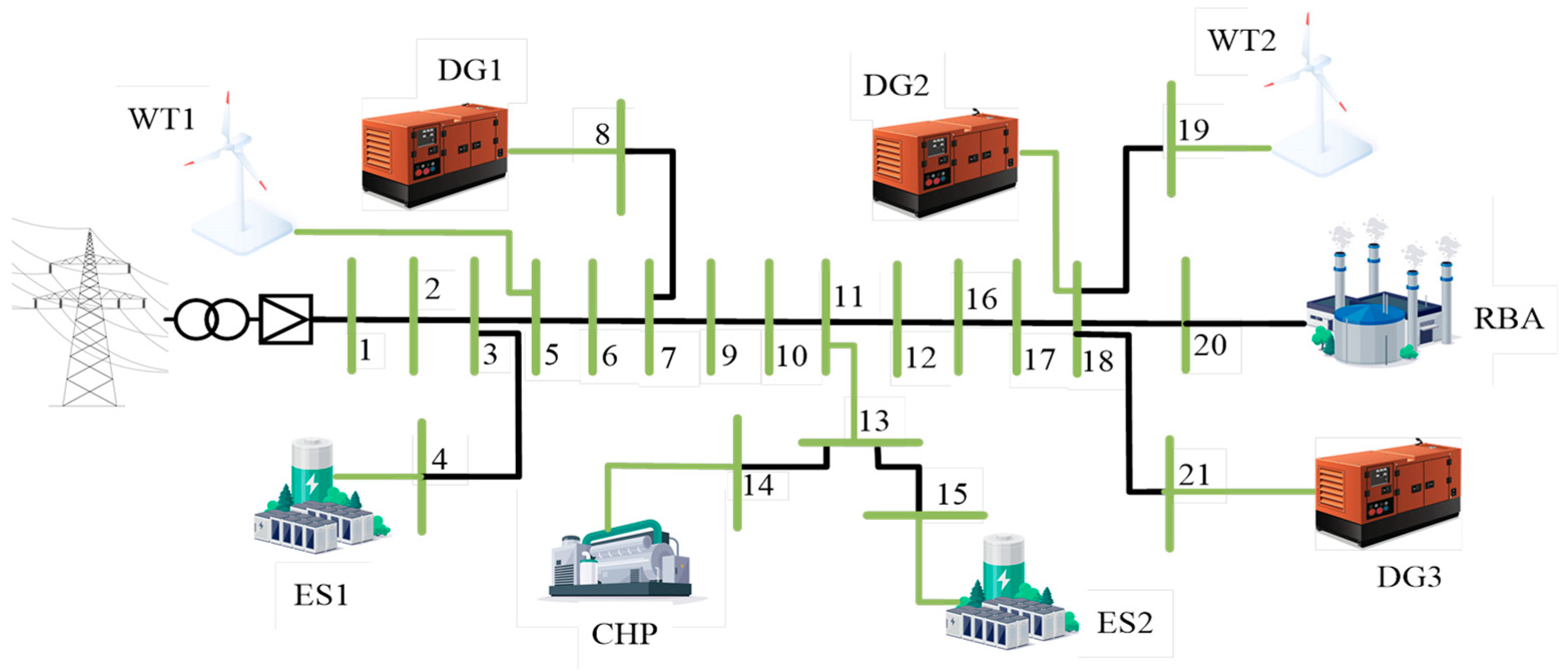
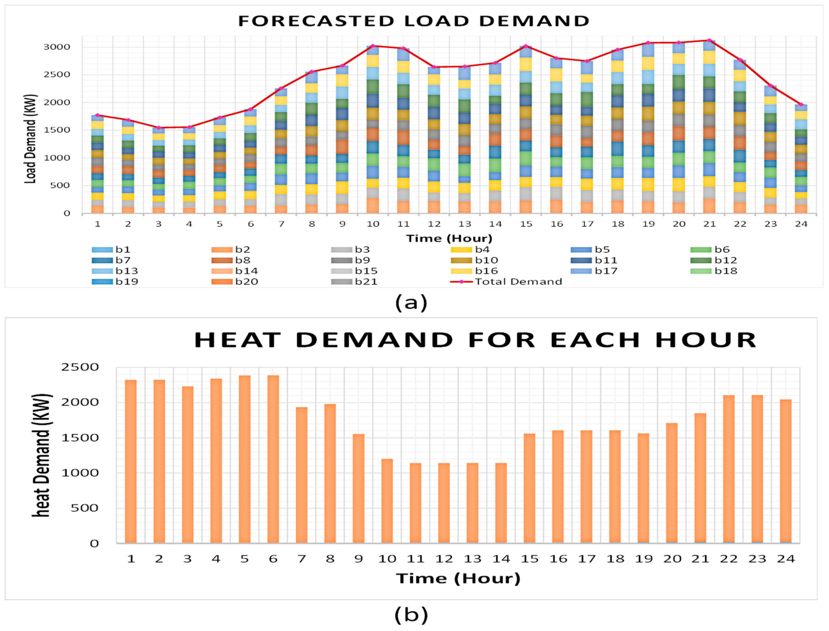
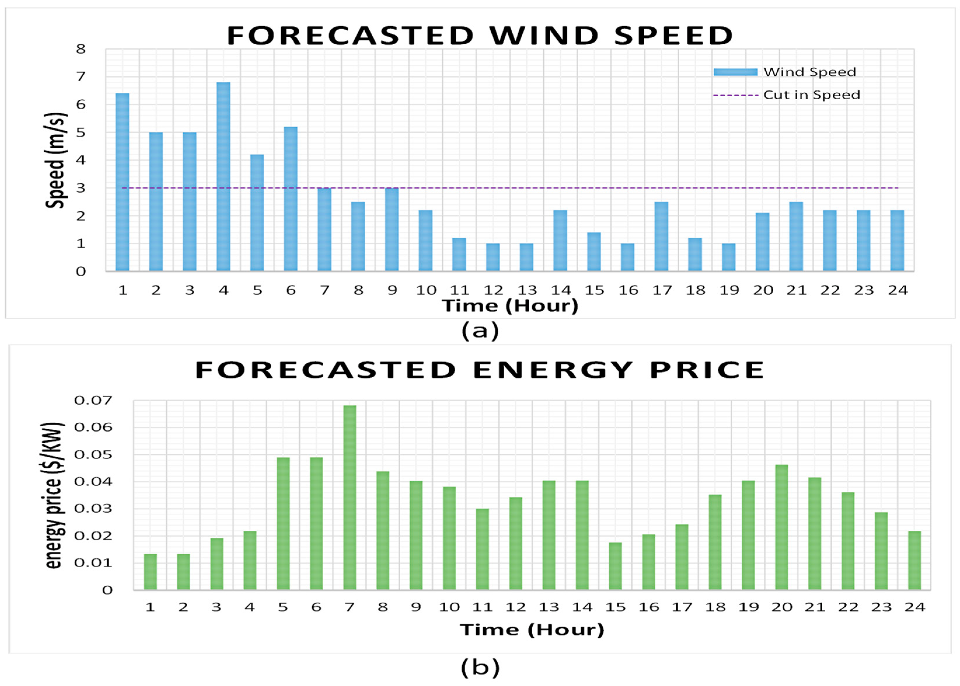
The total electrical power production must supply the load demand and power consumption of electrical vehicles each hour of the day. On the other hand, according to interruptible load, the delivery power can be less in some hours than the amount of demand.

$$\begin{gathered} {{\displaystyle \sum }}_d{P}_{d,t}^{DG}+{{\displaystyle \sum }}_h{P}_{h,t}^{CHP}+{{\displaystyle \sum }}_w{P}_{w,t}^w+{{\displaystyle \sum }}_r{P}_{r,t}^{RBA}+{{\displaystyle \sum }}_e{P}_{e,t}^{ES,DCH}-{{\displaystyle \sum }}_r{P}_{e,t}^{ES,CH}+P_t^{buy}= \\ (P_t^{load}-P_t^{IL})+{{\displaystyle \sum }}_v{P}_{v,t}^{EV} \end{gathered}$$

(47)

3. Simulation

3.1. Case Study Definition

To find the minimum value for the cost function, a network with three DG, two ES, one CHP, one RBA, and two WT is considered as shown in Figure 1. The proposed network is connected with the upstream network. Two hundred and ten electrical vehicles are located with PQ buses, and the information related to arrival, EV trade information, departure EV time, and initial charge is obtained from article 43. In addition, the main grid elements information is in

Table 2. DGs and CHP data.

DGs Data
Bus. No	$a_d^{DG}\left(\$/{\mathrm{KWh}}^2\right)$	$b_d^{DG}\left(\$/KWh\right)$	$c_d^{DG}\left(\$/h\right)$	$P_d^{DG,Max}\left(\mathrm{Kw}\right)$	$P_d^{DG,Min}\left(\mathrm{KW}\right)$	$SU{C}_d\left(\$\right)$
B8	2.4 $\times {10}^{-5}$	4.7 $\times {10}^{-5}$	1.9 $\times {10}^{-5}$	500	50	45
B18	2.4 $\times {10}^{-5}$	4.8 $\times {10}^{-5}$	2 $\times {10}^{-5}$	700	65	45
B21	2.6 $\times {10}^{-5}$	5 $\times {10}^{-5}$	2.3 $\times {10}^{-5}$	900	90	15
CHP Data
Bus. No	${\alpha }_h^{CHP}$	${\eta }_h^{Boiler}$	$f_h^{Boiler,\mathrm{MAX}}$	$f_h^{CHP,\mathrm{MAX}}$	$H_h^{\mathrm{S},\mathrm{MAX}}$	$H_{h,0}^{\mathrm{S}}$
B14	2	0.8	2000	2000	800	257

and

Table 3. ESs, RBA, and WTs data.

ES Data
Bus. No	${\mathsf{\eta }}_{\mathrm{e}}^{\mathrm{ES},\mathrm{CH}}$	${\mathsf{\eta }}_{\mathrm{e}}^{\mathrm{ES},\mathrm{DCH}}$	${\mathrm{P}}_{\mathrm{e}}^{\mathrm{MAX},\mathrm{CH}}$	${\mathrm{P}}_{\mathrm{e}}^{\mathrm{MAX},\mathrm{DCH}}$	${\mathrm{SOC}}_{\mathrm{e}}^{\mathrm{ES},\mathrm{MIN}}$	${\mathrm{SOC}}_{\mathrm{e}}^{\mathrm{ES},\mathrm{MIN}}$
B4	0.86	0.86	50	50	250	10
B15	0.86	0.86	150	150	750	50
RBA Data
Bus. No	${\propto }_{\mathrm{T}}^{\mathrm{RBA}}$	${\rho }^{RBA}$	$h{v}^{RBA}$	${\mathrm{P}}_{\mathrm{e}}^{\mathrm{RBA},\mathrm{Max}}$	${\mathrm{P}}_{\mathrm{e}}^{\mathrm{RBA},\mathrm{Min}}$	o
B20	0.3	0.02	0.51	50	6
WT Data
Bus. No	O&Mw	${\mathrm{Pw}}_{\mathrm{w}}^{\max }$	${ \mathrm{v}}_{\mathrm{w}}^{\mathrm{CIN}}$	${ \mathrm{v}}_{\mathrm{w}}^{\mathrm{R}}$	${ \mathrm{v}}_{\mathrm{w}}^{\mathrm{COUT}}$
B19	0.01	500	3	9	25
B5	0.01	500	3	9	25

. To solve the optimization problem, GAMS software version 28.2 and Cplex Solver have been used.

3.2. Uncertainty Modeling

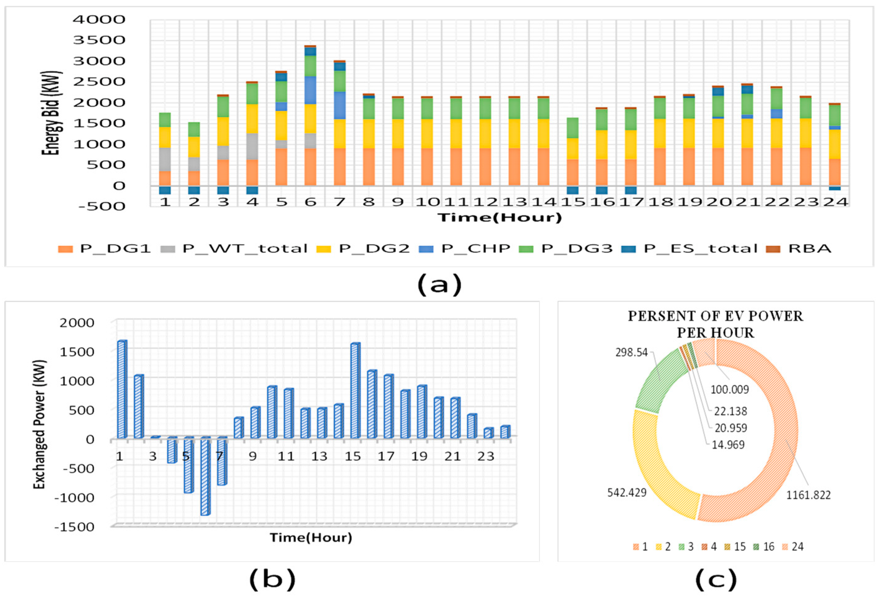
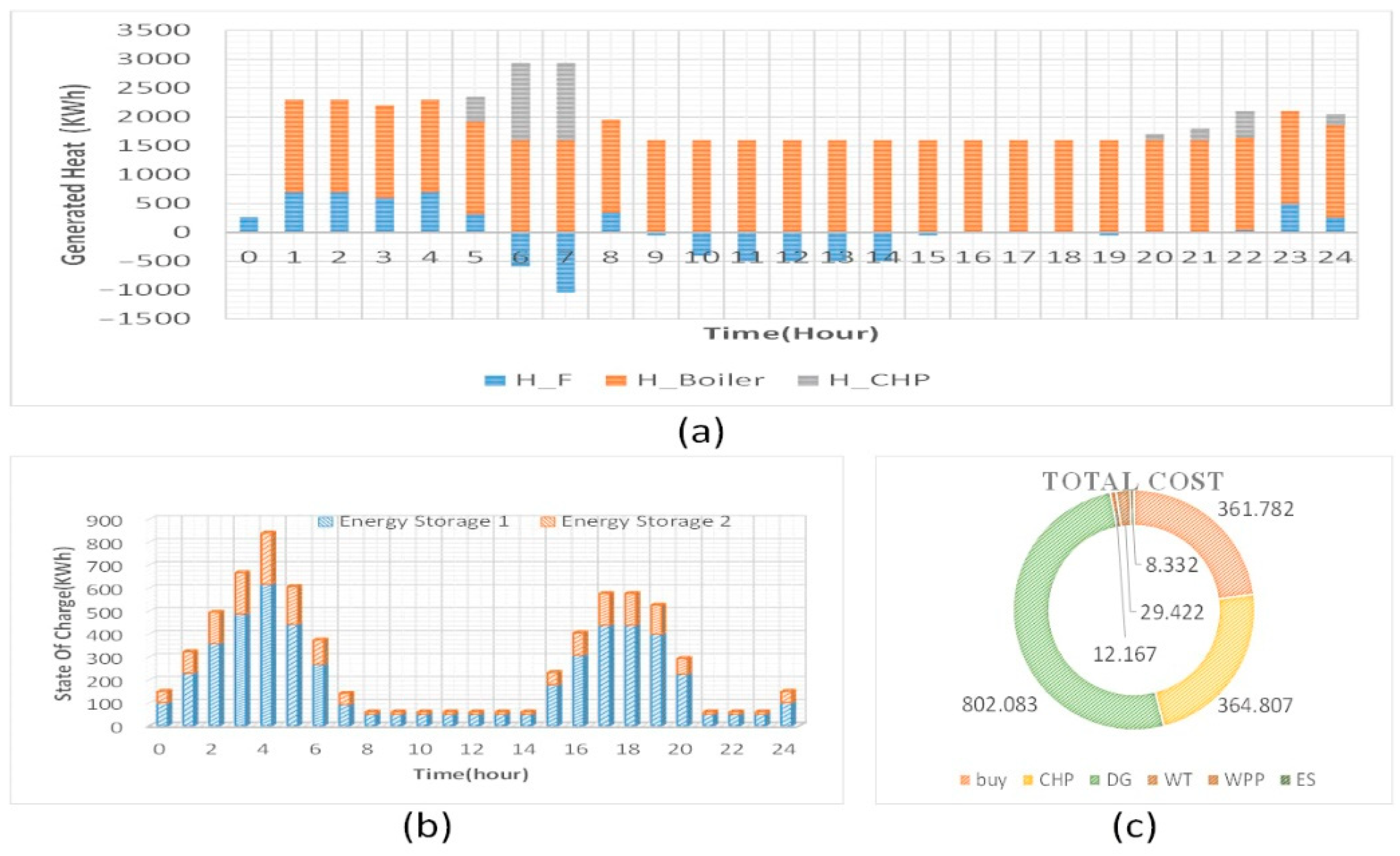
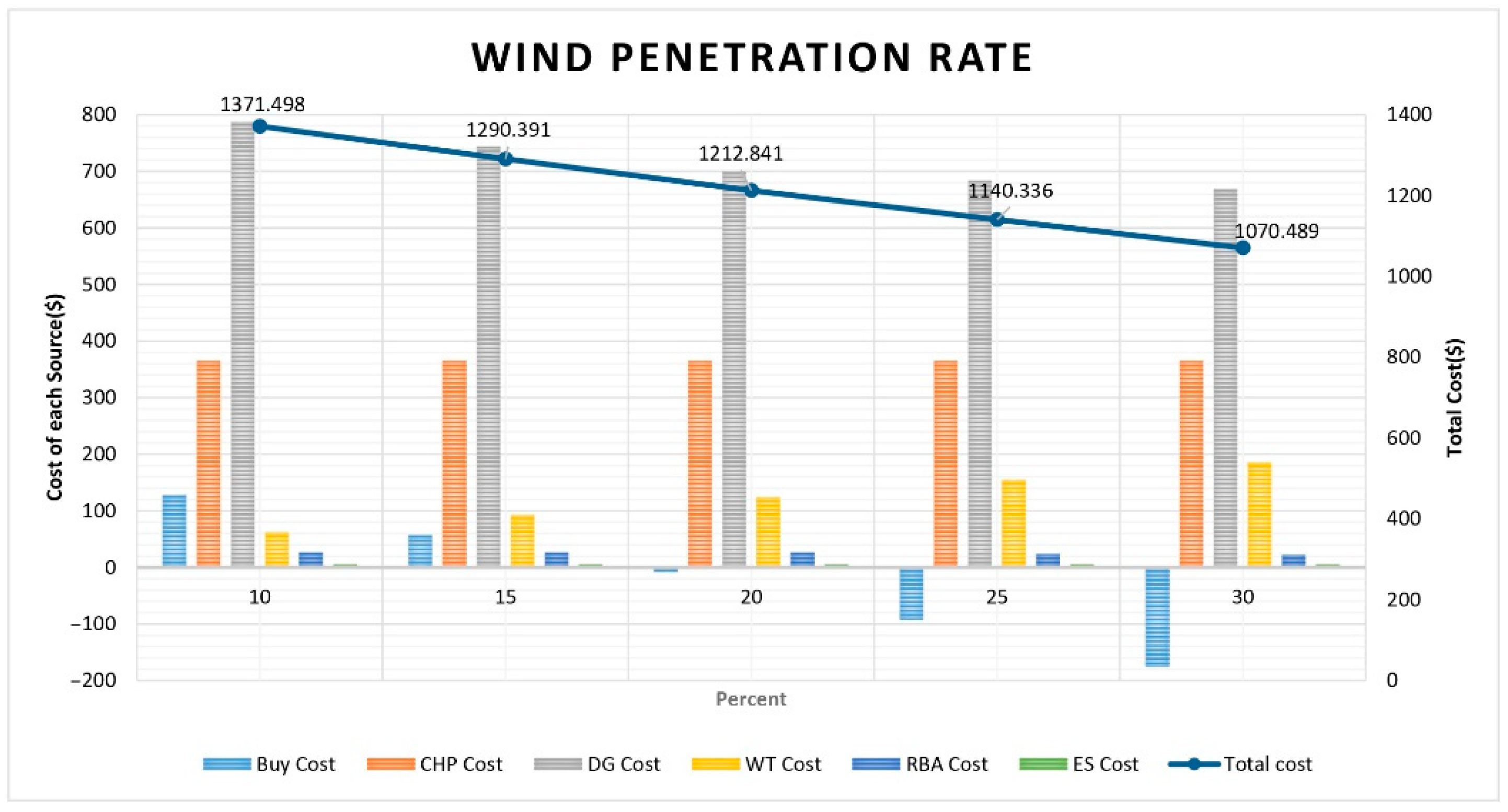
Recurrent neural networks (RNNs) are different from conventional neural networks in terms of functionality. This difference is that the information from the last moment affects the decision made in the current moment, so recurrent neural networks are used as one of the best options for predicting time data. Considering that the current consumption of the residential load is affected by the data of the last moment, the use of recurrent neural networks is a desirable solution. Because of the efficient nature of recurrent neural networks, there are vanishing limits and gradient explosions for long-term learning. The meaning of the disappearance of the gradient is the reduction of the soft gradient with the increase of the time interval, which leads to the convergence of the gradient towards zero. In addition, due to not normalizing the gradient in the learning process, it is possible to increase the gradient too much. To overcome these problems, Long-Short Term Memory (LSTM) neural networks have been created.

LSTM neural networks consist of three gates: forgetting, input, and output, which allow studying time series with a larger horizon. The forgetting gate and the input gate respectively determine the importance of the previous processing and the current input in the current processing, while the output gate will determine the result of the current processing. With reducing the size of system modeling, different stochastic parameters are becoming more important. It is not surprising that this issue is more crucial in MGs, which are also designed to operate in islanding mode. Consequently, in this paper the LSTM network, a promising tool in time series forecasting tasks, is utilized [25]. The general formulation of deep LSTM networks is presented in reference [24]. In this paper, the hourly data of Ontario province for electricity price, load demand, and wind speed for three years (1 January 2019, to 30 December 2021) are used as a dataset [26]. The previous 48-hour data are utilized to forecast each stochastic parameter. For the training, validation, and testing, the total dataset is divided into 80%, 10%, and 10%, respectively. The whole process of implementing LSTM networks is done in MATLAB software version 2019a by Deep Network Designer Toolbox [27]. The LSTM based forecasting framework shown is in Figure 2.

The day ahead forecasted electricity demand and heat demand are presented in Figure 3. In addition, the predicted electricity price and wind speed are shown in Figure 4.

3.3. Results

Figure 5a shows the components of the proposed microgrid, which includes the active production power of RBA, WT, DG, CHP, and the active power transmission of ES. Figure 5b shows the exchange of power between the upstream network and microgrid. Figure 5c shows the amount of accumulated energy absorbed by electrical vehicles. Due to low electricity price and low consumption load in the time period of 00.00 to 04.00, and availability of electrical vehicles and renewable energy production, charging and energy storage operations are carried out in ES. According to Figure 6b, SOC related to ES reaches its maximum value at the end of the period. From 00.00 to 02.00, the microgrid purchases energy from the upstream network to charge electrical vehicles. However, from 03.00 to 07.00, due to an increase in supply-to-demand ratio, the microgrid sells energy to the upstream network. With the rise in demand on the one hand and the decrease in wind turbine production, on the other hand, electricity is purchased from the upstream network from 08:00 to 00.00, and considering the high electricity price in the time above frame, electrical vehicles will not be charged.

Based on Figure 6b, the amount of SOC related to IS will reach its minimum value from 06.00 to 07.00 because the selling price is high in this period. Electrical vehicle charge and storage operations will be stopped before 15.00. In the time from 15.00 to 17.00, due to demand and price reduction of electricity, the energy storage process will be done in ES. In addition, the electrical vehicles which did not get charged in time period of 16.00 to 00.00, will be charged. The reasons for increase in electricity purchasing in time period of 15.00 to 17.00 are the charging of electrical vehicles and energy storage. In the time frame between 18.00 and 23.00, a load increase is observed, and by 22.00, consumption will have a downward trend. Figure 6a shows the amount of energy in the thermal storage and the boiler’s production power and CHP. The sum of energies in the three units mentioned above should supply the heat demand of the network. In addition, the CHP unit will produce electric power every hour along with thermal power supply, as shown in Figure 6a. Figure 6c shows the cumulative cost of energy storage and energy production sources. The suitable wind speed for generating electrical power (according to the shape of the wind speed) exists only in the period of 01.00 to 06.00. During the remaining hours of the day, DG will be in the network, so DG will include a large share of the final cost.

Examining the sensitivity of electricity prices to the penetration rate of renewable energy sources is vital due to the desire to replace fossil fuels. The sensitivity of the production cost of each energy production source and the total cost of energy production in the microgrid to the penetration rate of renewable energy sources is shown in Figure 7. The proposed optimal model has been implemented each time to manage different operational strategies with different input parameters. According to Figure 7, changing the wind energy penetration coefficient has been used to check the sustainability of the proposed network. The cost associated with generating energy from distributed generation sources and energy purchased from the upstream grid will decrease with increasing penetration. On the other hand, the maintenance cost of the wind turbine will clearly increase with the increase in production. In addition, the cost of production by other energy sources will change little. The reason for this is the increase in the sale of electrical energy to the upstream network and the decrease in the need for energy production by scattered production sources. Therefore, the total cost of energy production will decrease almost linearly.

4. Conclusions

This study presented an energy management system (EMS) for a microgrid consisting of DG, ES, wind turbine, EVs, RBA, and CHP. To obtain a suitable model for estimating the amount of wind turbine production based on meteorological data, the amount of the day ahead load, and electricity price, the LSTM network has been employed.

To achieve the global optimal point, the model must be linearized with the help of the piecewise linear method. The final cost of energy production in the state of connection to the grid is $1549.35. The share of the highest cost among energy production sources (with 51% of the total cost) is related to the diesel generator. In addition, the effect of increasing the penetration rate of renewable energies on the total Cost has been investigated. By increasing the penetration coefficient of wind energy up to 30% of the total power, the total cost will be reduced by 30.9%.

References

1. Kamarposhti, M.A.; Colak, I.; Eguchi, K. Optimal energy management of distributed generation in micro-grids using artificial bee colony algorithm. Math. Biosci. Eng. 2021, 18, 7402–7418. [Google Scholar] [CrossRef] [PubMed]
2. Fan, S.; He, G.; Zhou, X.; Cui, M. Online Optimization for Networked Distributed Energy Resources with Time-Coupling Constraints. IEEE Trans. Smart Grid 2020, 12, 251–267. [Google Scholar] [CrossRef]
3. Guo, C.; Wang, X.; Zheng, Y.; Zhang, F. Real-time optimal energy management of microgrid with uncertainties based on deep reinforcement learning. Energy 2021, 238, 121873. [Google Scholar] [CrossRef]
4. Raghav, L.P.; Kumar, R.S.; Raju, D.K.; Singh, A.R. Optimal Energy Management of Microgrids Using Quantum Teaching Learning Based Algorithm. IEEE Trans. Smart Grid 2021, 12, 4834–4842. [Google Scholar] [CrossRef]
5. Javed, M.S.; Song, A.; Ma, T. Techno-economic assessment of a stand-alone hybrid solar-wind-battery system for a remote island using genetic algorithm. Energy 2019, 176, 704–717. [Google Scholar] [CrossRef]
6. Erenoğlu, A.K.; Şengör, I.; Erdinç, O.; Taşcıkaraoğlu, A.; Catalão, J.P. Optimal energy management system for microgrids considering energy storage, demand response and renewable power generation. Int. J. Electr. Power Energy Syst. 2021, 136, 107714. [Google Scholar] [CrossRef]
7. Gupta, N.; Khosravy, M.; Patel, N.; Dey, N.; Mahela, O.P. Mendelian evolutionary theory optimization algorithm. Soft Comput. 2020, 24, 14345–14390. [Google Scholar] [CrossRef]
8. Gupta, N.; Khosravy, M.; Gupta, S.; Dey, N.; Crespo, R.G. Lightweight Artificial Intelligence Technology for Health Diagnosis of Agriculture Vehicles: Parallel Evolving Artificial Neural Networks by Genetic Algorithm. Int. J. Parallel Program. 2020, 50, 1–26. [Google Scholar] [CrossRef]
9. Variengien, A.; Pontes-Filho, S.; Glover, T.E.; Nichele, S. Towards Self-organized Control: Using Neural Cellular Automata to Robustly Control a Cart-Pole Agent. Innov. Mach. Intell. 2021, 1, 1–14. [Google Scholar] [CrossRef]
10. Dashtdar, M.; Bajaj, M.; Hosseinimoghadam, S.M.S. Design of Optimal Energy Management System in a Residential Microgrid Based on Smart Control. Smart Sci. 2021, 10, 25–39. [Google Scholar] [CrossRef]
11. Adefarati, T.; Bansal, R.; Bettayeb, M.; Naidoo, R. Optimal energy management of a PV-WTG-BSS-DG microgrid system. Energy 2020, 217, 119358. [Google Scholar] [CrossRef]
12. Aghdam, F.H.; Kalantari, N.T.; Mohammadi-Ivatloo, B. A chance-constrained energy management in multi-microgrid systems considering degradation cost of energy storage elements. J. Energy Storage 2020, 29, 101416. [Google Scholar] [CrossRef]
13. Faghiri, M.; Samizadeh, S.; Nikoofard, A.; Khosravy, M.; Senjyu, T. Mixed-Integer Linear Programming for Decentralized Multi-Carrier Optimal Energy Management of a Micro-Grid. Appl. Sci. 2022, 12, 3262. [Google Scholar] [CrossRef]
14. Jia, S.; Kang, X. Multi-Objective Optimal Scheduling of CHP Microgrid Considering Conditional Value-at-Risk. Energies 2022, 15, 3394. [Google Scholar] [CrossRef]
15. Shayegan-Rad, A.; Badri, A.; Zangeneh, A. Day-ahead scheduling of virtual power plant in joint energy and regulation reserve markets under uncertainties. Energy 2017, 121, 114–125. [Google Scholar] [CrossRef]
16. Najafi-Ghalelou, A.; Zare, K.; Nojavan, S. Optimal scheduling of multi-smart buildings energy consumption considering power exchange capability. Sustain. Cities Soc. 2018, 41, 73–85. [Google Scholar] [CrossRef]
17. Gougheri, S.S.; Jahangir, H.; Golkar, M.A.; Ahmadian, A.; Golkar, M.A. Optimal participation of a virtual power plant in electricity market considering renewable energy: A deep learning-based approach. Sustain. Energy Grids Netw. 2021, 26, 100448. [Google Scholar] [CrossRef]
18. Bahmani, R.; Karimi, H.; Jadid, S. Stochastic electricity market model in networked microgrids considering demand response programs and renewable energy sources. Int. J. Electr. Power Energy Syst. 2019, 117, 105606. [Google Scholar] [CrossRef]
19. Mazidi, M.; Rezaei, N.; Ardakani, F.J.; Mohiti, M.; Guerrero, J.M. A hierarchical energy management system for islanded multi-microgrid clusters considering frequency security constraints. Int. J. Electr. Power Energy Syst. 2020, 121, 106134. [Google Scholar] [CrossRef]
20. Du, Y.; Li, F. Intelligent Multi-Microgrid Energy Management Based on Deep Neural Network and Model-Free Reinforcement Learning. IEEE Trans. Smart Grid 2019, 11, 1066–1076. [Google Scholar] [CrossRef]
21. Tan, B.; Chen, H. Multi-objective energy management of multiple microgrids under random electric vehicle charging. Energy 2020, 208, 118360. [Google Scholar] [CrossRef]
22. Jani, A.; Karimi, H.; Jadid, S. Multi-time scale energy management of multi-microgrid systems considering energy storage systems: A multi-objective two-stage optimization framework. J. Energy Storage 2022, 51, 104554. [Google Scholar] [CrossRef]
23. Gougheri, S.S.; Jahangir, H.; Golkar, M.A.; Moshari, A. Unit Commitment with Price Demand Response based on Game Theory Approach. In Proceedings of the 2019 International Power System Conference (PSC), Tehran, Iran, 9–11 December 2019; pp. 234–240. [Google Scholar] [CrossRef]
24. Sadeghi, S.; Jahangir, H.; Vatandoust, B.; Golkar, M.A.; Ahmadian, A.; Elkamel, A. Optimal bidding strategy of a virtual power plant in day-ahead energy and frequency regulation markets: A deep learning-based approach. Int. J. Electr. Power Energy Syst. 2020, 127, 106646. [Google Scholar] [CrossRef]
25. Jahangir, H.; Gougheri, S.S.; Vatandoust, B.; Golkar, M.A.; Golkar, M.A.; Ahmadian, A.; Hajizadeh, A. A Novel Cross-Case Electric Vehicle Demand Modeling Based on 3D Convolutional Generative Adversarial Networks. IEEE Trans. Power Syst. 2021, 37, 1173–1183. [Google Scholar] [CrossRef]
26. Power Data. Available online: http://www.ieso.ca/power-data (accessed on 3 November 2022).
27. Little, J.; Moler, C. Statistics and Machine Learning Toolbox; Version 9.6 (R2019a); MathWorks: Natick, MA, USA, 2019. [Google Scholar]
Figure 1. Proposed network diagram.
Sustainability 14 15036 g001
Figure 2. The LSTM based forecasting framework.
Sustainability 14 15036 g002
Figure 3. Electricity and heat demands. (a) Hourly forecasted electricity demand curve. (b) Hourly heat demand curve.
Sustainability 14 15036 g003
Figure 4. Day-ahead prediction of stochastic parameters. (a) Hourly forecasted wind speed curve. (b) Hourly predicted energy price curve.
Sustainability 14 15036 g004
Figure 5. Numerical result of the proposed solution. (a) The amount of production power for each unit of microgrid components. (b) Exchanged power between the microgrid and upstream network. (c) Power is absorbed by electrical vehicles in hours.
Sustainability 14 15036 g005
Figure 6. (a) Heat generation by heat storage, boiler, and CHP to provide heat demand. (b) State of charge for each ES unit. (c) The power production cost of each unit.
Sustainability 14 15036 g006
Figure 7. The sensitivity of the production cost and the total cost of energy production in the microgrid to the penetration rate of RERs.
Sustainability 14 15036 g007