Article

High-Frequency Monitoring to Estimate Loads and Identify Nutrient Transport Dynamics in the Little Auglaize River, Ohio

1
School of Environment and Natural Resources, The Ohio State University, Columbus, OH 43210, USA
2
Department of Evolution, Ecology, and Organismal Biology, The Ohio State University, Columbus, OH 43210, USA
3
Office for Research and Graduate Education, The Ohio State University, Columbus, OH 43210, USA
4
Ohio State University Extension, The Ohio State University, Columbus, OH 43210, USA
*
Author to whom correspondence should be addressed.
Sustainability 2022, 14(24), 16848; https://0-doi-org.brum.beds.ac.uk/10.3390/su142416848
Submission received: 16 November 2022 / Revised: 9 December 2022 / Accepted: 10 December 2022 / Published: 15 December 2022
(This article belongs to the Special Issue Prospects in Sustainable Water Management)

Abstract

:
New technologies allow for the in situ monitoring of nutrients, specifically nitrogen and phosphorus, in water systems at increasingly higher temporal frequencies. These technologies allow for the near-continuous monitoring of water quality, which can potentially provide new perspectives on temporal variations in nutrient concentrations and transport dynamics, ultimately supporting more targeted and sustainable water management. The current study investigated the utility of monitoring nitrate-N and soluble reactive phosphorus (SRP) in situ using wet analytical chemistry for one year at 2-h intervals in a small agricultural watershed located in northwestern Ohio. While we saw large variability in the estimated nutrient loads due to daily variations in the high-temporal resolution nutrient concentrations, the nutrient loads were fundamentally driven by high-flow events for this agricultural watershed. Concentration–discharge relations were then developed to help identify how nutrients are stored and released over time scales ranging from low-flow seasonal responses to event-driven high-flow storms. The patterns in the concentration–discharge relations indicated a potential shift in the timing of the mobilization responses for SRP at the event scale over the course of the year. These results suggest that SRP-targeted management practices would need to intercept the dominant delivery pathways of phosphorus in the watershed, such as the tile drainage runoff, to help reduce phosphorus loading. For nitrate-N, patterns in the concentration–discharge relations revealed an increased mobilization response, which was seen during the growing season with low-flow conditions, indicating the potential role of biological uptake instreams across the lowest flows and concentrations of the year. Collectively, high-frequency temporal nutrient data monitored over individual events and across seasons offer guidance for management decisions while allowing us to track progress toward water quality goals.

1. Introduction

Water quality in agricultural landscapes, particularly in response to excess nutrient inputs of nitrogen and phosphorus, has become an increasing focus of concern for water resource management. Excess nutrients in runoff from agricultural systems ultimately drain into waterbodies, such as the surrounding streams and rivers, expediting eutrophication, harmful algal blooms (HABs), and general impairment in downstream waterbodies [1,2]. Water quality monitoring is typically conducted within freshwater systems with the goals of better understanding the impact of agricultural and other activities in watersheds and informing the management of nutrients in agricultural runoffs across scales. Despite the clear need for monitoring, collecting water samples to characterize nutrient concentrations can be expensive, time-consuming, and, especially in high-flow events, not always possible. Watershed managers, thus, need to make decisions as to what sampling methods and frequencies will give the most representative information with the least amount of observational error and ambiguity.
Research has demonstrated that the choices made around sampling methods and frequencies—whether the choice is about the sampling location, the collection process, the discharge measurements, the overall sampling frequency throughout time, the calculations used, or the laboratory analysis selected [2,3,4]—can have a clear impact on how we characterize water quality and prescribe subsequent management strategies. For example, the sampling methods and frequencies have significant impacts on how we characterize nutrient loads in watersheds. Nutrient loads are calculated as the products of discharge measurements and nutrient concentrations. Watershed managers continue to look for the most efficient, cost-effective, and accurate ways to characterize nutrient loads [5]. In the long term, lower frequency records are often used to characterize nutrient loads [6]. Load estimations can vary based on the length of a study [7], the underlying geology of a study site [8], the high-flow or storm response rates [5], the size of a watershed [3], or the focus nutrient type [2]. With all that said, calculating nutrient loads that are as accurate and precise as possible remains crucial for understanding and implementing the best management practices (BMPs) and decisions [9].
To that end, new technologies are constantly being developed to support the continuous and in situ monitoring of nutrient concentrations in freshwater systems [10]. These technologies often rely on either optical sensors or in-field wet analytical chemistry to measure nutrient concentrations [11]. For nitrate-N, optical sensors for monitoring high-frequency concentrations are becoming more common; however, optical sensor technology does not exist for the high-frequency monitoring of phosphorus concentrations. Monitoring phosphorus conditions currently requires wet-chemistry techniques, whether in the laboratory or in situ, which can be considered an impediment for monitoring phosphorus over a range of flow conditions. Regardless of the technology that is being utilized, there is an inherent need to compare new technologies to traditional monitoring schemes and laboratory-derived concentrations. Further, as new technologies become available that make it possible to observe both nitrogen and phosphorus concentrations in situ in near real-time over extended durations, there is a continued need to assess what high-frequency data reveal about the transport dynamics of nitrogen and phosphorus.
Technological advancements in water monitoring and increased access to high-resolution chemistry data have also promoted renewed interest in water quality assessment tools, such as establishing concentration–discharge (C–Q) relations and, subsequently, assessing their value in characterizing catchment storages, time lags, and legacy effects when comparing between event and seasonal responses [12]. For example, to distinguish between seasonal C–Q relations and event-based C–Q relations for phosphorus and nitrate-N, 219 French catchments were used to characterize the nutrient dynamics for systems covering a wide range of soils, climates, and land use characteristics [13]. Often, the differences between long-term and event-based C–Q responses indicate different controls on solute transport and storage processes on different temporal scales [6]. At the daily scale, for example, Welikhe et al. [14] saw that C–Q patterns could be linked to the soil P status because a chemostatic response was observed for streams that drain soils that serve as a P source and a dilution behavior was observed for areas that drain primarily P sink soils. Such linkages can be informative as managers seek to implement practices across a watershed to support nutrient retention in the landscape and reduce downstream loading.
From a sustainable water management perspective, understanding the processes that control nutrient losses from agricultural landscapes is essential to better define critical source areas and inform conservation practice recommendations [14]. Welikhe et al. [14] further highlighted the need for higher temporal resolution monitoring data to increase the understanding of nutrient loss patterns (explicitly phosphorus) and to better inform/guide water resource managers, who are tasked with improving the water quality conditions. The recent advances in in situ water quality monitoring with optical sensors and wet chemistry analyzers [1,11,15,16] can help to bridge this gap in high-temporal resolution nutrient data. To this end, the objective of this current study is to demonstrate the potential use of high-frequency (here, sampling every 2 h) in situ wet-chemistry analysis for the determination of nitrate-N and soluble reactive phosphorus (SRP) concentrations. Specifically, we used one year of monitoring from the GreenEyes NuLab autonomous nutrient analyzer (NuLab) to characterize both high-flow storm event and low-flow seasonal nutrient responses for a small agricultural watershed facing severe water quality problems through the lens of load estimations and concentration–discharge (C–Q) relations. We hypothesize that comparing individual storm and seasonal low-flow period nutrient loads and C–Q relations will allow for the targeting of the best management strategies for reducing nutrient loads. Our study is novel as we are among the first to explore the value that is added through high-temporal resolution nitrate-N and SRP observations over seasonal variations with regards to understanding water quality variations with implications for sustainable water management. This exploration is important as it can helphi water resource managers decide if the investment in high-temporal resolution observations is relevant for their needs, while at the same time familiarizing researchers with what these types of data can offer with regards to analyses in real-world settings.

2. Materials and Methods

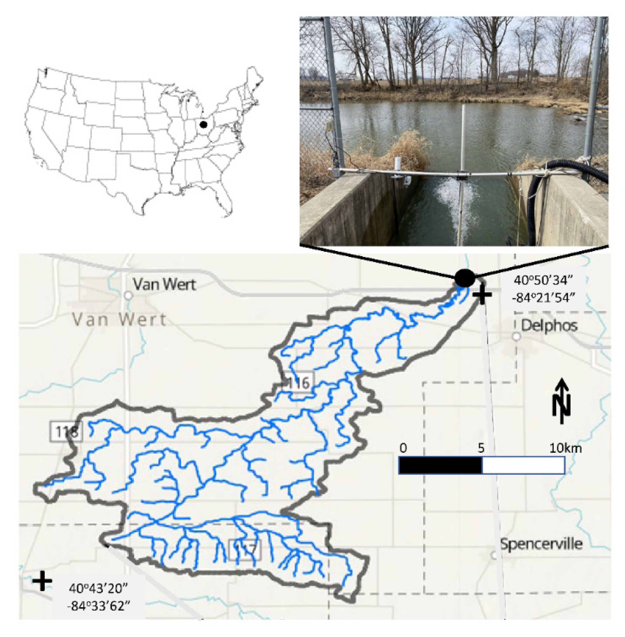
2.1. Site Description

The Little Auglaize River, located in northwestern Ohio, has a watershed covering 197 km2 with land use that consists of 88.5% agriculture (cultivated crops), 4.6% forest, and 6.9% developed land (Figure 1). The long-term mean annual precipitation is 99 cm for this watershed, according to the National Land Cover Database from the U.S. Geological Survey. As with most of the region, agriculture is the primary land use in the watershed and consists primarily of corn and soy production. Corn and soy are planted early, around mid-May, and harvested by mid-October. Tile drainage structures are common throughout the area due to the underlying geology (predominantly glacial tills) and poorly draining soils [17].
The Little Auglaize River provides water to the Delphos Gillmor reservoir, which serves as the sole source of drinking water passing through traditional water treatment facilities for the city of Delphos, Ohio, and more than 7000 people. At the location of the water intake for the Delphos Gillmor reservoir (40°52′51.9″ N, 84°22′05.9″ W), the Little Auglaize River is currently classified as impaired by the U.S. Environmental Protection Agency for nitrate-N, algae, and Escherichia coli. In addition, the Dry Fork tributary of the Little Auglaize River is the only hydrologic unit code (HUC) 12 watershed, ranging in size from about 4 to 16 hectares, in Ohio with both nitrate-N and cyanotoxin drinking water impairments (at Delphos) and was one of the highest ranked Maumee River HUC 12 watersheds on the Ohio EPA’s 305(d) list of impaired watersheds. The source water nitrate-N concentrations have been as high as 16 mg/L (the drinking water standard is 10 mg/L) and have impacted the Delphos water system’s ability to fill their reservoir and maintain an adequate supply. Ohio’s 2020 Domestic Action Plan also estimates that a phosphorus reduction of 28,600 pounds is needed annually in the Little Auglaize watershed to help meet the current Lake Erie phosphorus targets to achieve a 40% reduction in the spring total and soluble reactive phosphorus loads to Lake Erie [18].

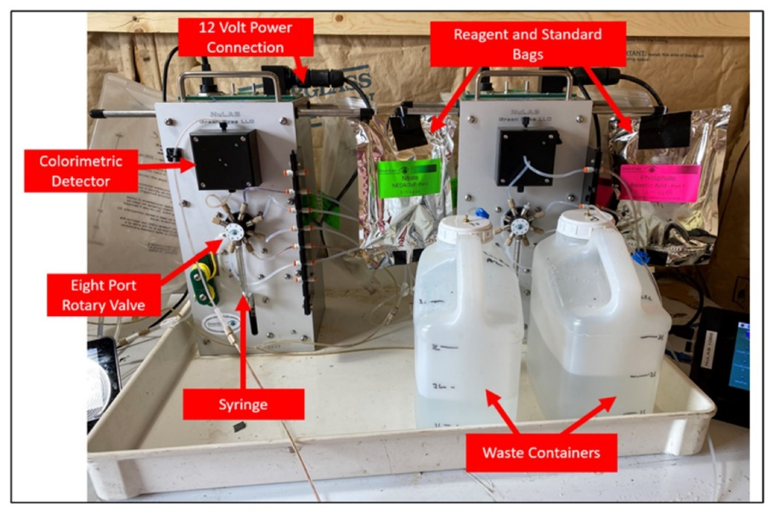
2.2. In Situ Nutrient Monitoring

The Greeneyes NuLab autonomous nutrient analyzer (NuLab) (Figure 2) was installed at the reservoir intake to characterize the nutrient loads to the Delphos reservoir and help determine when the Gillmor reservoir can safely be filled. The Ohio State University Water Quality Extension was responsible for the operation and maintenance of the NuLab for the period between February 2021 and January 2022 to complete one full year of high-frequency nutrient data collection. The NuLab is an automated wet-chemistry, multi-constituent analyzer that has the capability to analyze water samples for dissolved nutrient concentrations, including nitrate-N plus nitrite, nitrite, soluble reactive phosphorus (SRP), ammonia, and silicate. The NuLab is controlled by a Raspberry Pi Linux-based computer that can be programmed at a sampling frequency as low as one sample every two hours. The NuLab utilizes a colorimetric detector that shines filtered light through flow cells, allowing for concentration quantifications by a photodiode aligned with the available standard methods. The NuLab for our study was set up with remote communication for real-time data transmission and was powered by a 120 V power supply. For our monitoring, two nutrient analyzers were installed with detectors for specifically SRP (0.005 mg/L detection limit) and nitrate-N plus nitrite (0.01 mg/L detection limit).
The water sampling consisted of water collection from the reservoir intake via an automated submersible pump that was drawing and filtering water for the subsequent analyses. Prior to processing each water sample, the NuLab processes a nutrient-specific on-board standard, which serves as a system performance indicator. Each NuLab analysis had a designated protocol to process and run the on-board standard and nutrient-specific reagents (NEDA/sulfa and imidazole for nitrate-N; molybdic acid and ascorbic acid for SRP). The inlet channel was flushed prior to running each sample. The values produced by the onboard standards and reagents were then used to calibrate the subsequent sample concentrations. For our study, the nitrate-N on-board standard had a mean of 0.167 mg/L and a standard deviation of 0.130 mg/L. The phosphate on-board standard had a mean of 0.084 mg/L with a standard deviation of 0.037 mg/L.

2.3. Nutrient Data Quality Control

Over the course of our one-year study, the NuLab collected and analyzed a total of 4380 samples each for SRP and nitrate-N. However, equipment malfunctions reduced these useable results to 3736 (85% of the total possible) and 3624 (83% of the total possible) for nitrate-N and SRP, respectively. These remaining data were subjected to a relatively simple data quality assessment and control to identify suspected low and high values. Here, we opted for a simple approach based on absolute values to avoid potential overprocessing or over smoothing of the initial raw data that was returned from the NuLab. For the low values, we used a lower threshold for the data quality control, which was set at zero to remove any erroneous negative concentrations for nitrate-N and SRP. Based on this low threshold, 1.7% and 10.0% of the total NuLab reported data were removed for nitrate-N and SRP, respectively. High thresholds were set for both the nitrate-N and SRP data at three standard deviations from the mean for each dataset, namely 16.9 mg/L for nitrate-N and 1.0 mg/l for SRP. Based on these high thresholds, 2.0% and 0.5% of the total NuLab data were removed for nitrate-N and SRP, respectively. A total of 3.7% and 10.5% of the total possible nitrate-N and SRP data were removed because of equipment malfunctions or violations of the data quality thresholds and were not made available for subsequent analyses.

2.4. Rainfall and Discharge Monitoring

Daily precipitation data were collected from the Community Collaborative Rain, Hail and Snow Network (CoCoRaHS) station OH-AL-8, which is approximately 7 km from the reservoir intake [19]. A pressure transducer was deployed at the reservoir intake to record the stream stage (H), which was subsequently converted to discharge (Q) using a rating curve that was developed for the site (Q = 24.8H2 − 3.9H + 0.2; R2 = 0.99; p < 0.05; n = 8). The discharge was estimated at the same temporal resolution (e.g., 2 h) as the NuLab data by averaging 15-min discharge estimates. A double mass curve of the cumulative daily precipitation and the cumulative daily discharge was used to assess the consistency between the rainfall–runoff relations for the watershed throughout the study period.

2.5. Nutrient Load Estimations

The nutrient loads were calculated on a two-hour frequency using Equation (1) as follows:
L i = C i Q i
where Li is the instantaneous load for the sample interval i, Ci is the instantaneous concentration measured by the NuLab, and Qi is the instantaneous discharge [2]. The cumulative nutrient loads were calculated by multiplying Li by the designated time interval (two hours for the high-frequency data) and cumulatively summing the loads throughout the record period. Of course, some data gaps existed in the high-frequency datasets, where measurements were not collected by the NuLab instrument or where the data points were removed by the quality control thresholds. The gaps in the estimated nutrient load timeseries were filled using the applicable monthly averages for nitrate-N and SRP to allow for continuous load estimations over the entire period. While other gap-filling approaches exist, the monthly averages were selected as a simple method that would have minimal impact on subsequent results and interpretation.
The high-frequency nutrient load estimation was then assumed to represent the “true” annual nutrient load for the Little Auglaize River. To test the impact of the temporal data frequency, or sampling interval, the maximum and minimum daily and weekly instantaneous concentrations were extracted for nitrate-N and SRP and used to represent sampling occurring once daily or once weekly, respectively. These concentration values were paired with the two-hour frequency discharge, and the load calculations were completed using Equation (1). The cumulative loads were calculated for the daily and weekly values by multiplying the instantaneous load by the necessary period and summing the load values throughout the record period. As the maximum and minimum concentrations were selected, these cumulative load estimates can be thought of as the highest and lowest possible values for the Little Auglaize River as a function of the daily or weekly sampling.

2.6. Concentration–Discharge Relations

Concentration–discharge (C–Q) plots were used to assess the potential for chemostatic versus diluting or mobilizing responses, collectively known as the export pattern, of nitrogen and phosphorus across the high-flow events and low-flow periods for the watershed. C–Q plots were developed in the log–log space for the two-hour interval nitrate-N and SRP concentrations plotted against the associated discharge. The power law relations, which are linear in the log–log space and are frequently used to describe the C–Q relations in smaller watersheds with high-frequency data [20], were determined from the C–Q data using the following equation:
C = a Q b
where C is the concentration, Q is the discharge, and a and b correspond to the intercept and slope of the linear equation in the log–log space. Following the definitions put forward by Godsey et al. [21], the C–Q relations with negative slopes (b < −0.1) indicate a dilution response, with the concentrations decreasing as the discharge increases. The C–Q relations with positive slopes (b > 0.1) indicate a mobilization response, with the concentrations increasing as the discharge increases. The C–Q relations with slopes near zero (−0.1 < b < 0.1) indicate a more chemostatic response, such that the concentration tends to remain stable regardless of the discharge.
The C–Q relations for both nitrate-N and SRP can be highly non-linear over time (e.g., [13,22]); therefore, various subsets of data were defined to isolate potential differences in the C–Q relations under different seasons and conditions. For example, high-flow data subsets were created by selecting periods where the discharge was greater than the 90th percentile for our observation period. These periods corresponded to the largest precipitation-impacted discharge events for the watershed. The high-flow data were then split into individual storm events, where (1) the peak discharge at least doubled from the observed pre-storm discharge and (2) nitrate-N or SRP data were available [6]. The remaining low-flow data (e.g., Q < 90th percentile) were split into two categories: non-growing season (data collected before mid-May or after mid-October) and growing season (data collected between mid-May and mid-October). Here, the growing season was defined based on knowledge of the area and confirmed by the physical pattern in the double-mass curve.
With regards to the statistical analysis, the power law relations (Equation (2)) were fit as linear regressions to the various subsets of the C–Q relations in the log–log space using the lm.r package in R [23]. Standard F-tests were used to assess the significance of the linear regression models, and a p-value of < 0.05 was assumed to be significant. We used the slopes of these linear regressions to characterize the C–Q relations considered.

3. Results

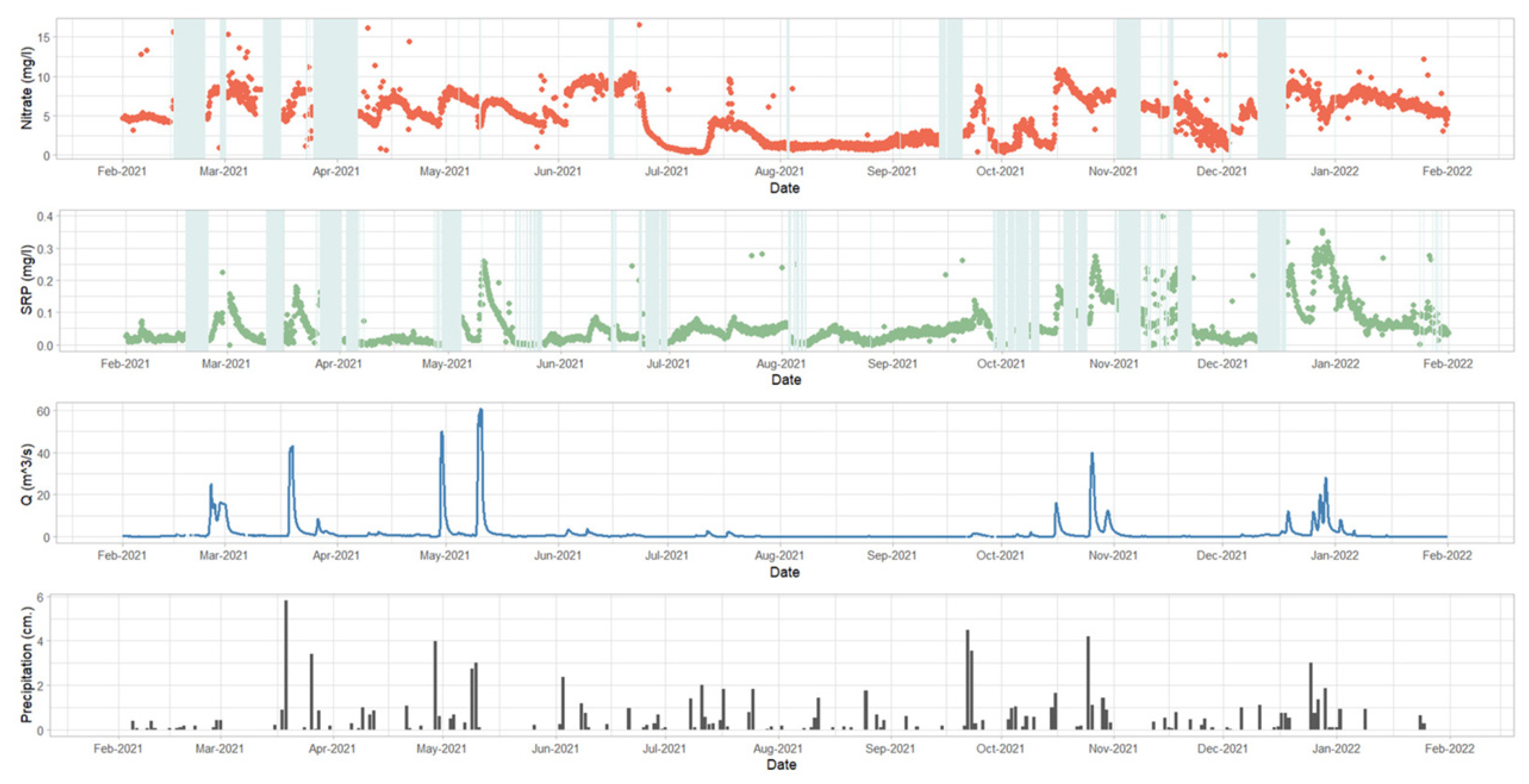
3.1. High-Frequency Nutrient Monitoring

Over the year of monitoring, the nitrate-N values ranged from 0.34 to 16.56 mg/L, with a mean of 4.80 mg/L and a standard deviation of 4.07 mg/L. The nitrate-N values were at their lowest during the late growing season months of July, August, and September, with monthly averages of 2.27, 1.24, and 2.89 mg/L, respectively (Figure 3). The SRP values ranged from 0.005 to 0.398 mg/L, with a mean of 0.030 mg/L and a standard deviation of 0.325 mg/L. The SRP values peaked during storm events and were less than 0.1 mg/L during the lowest discharge periods (Figure 3). Diurnal fluctuations were obvious during lower discharges, especially during the growing season. The diurnal concentration fluctuations ranged up to 1.00 mg/L for nitrate-N and 0.040 mg/L for SRP.

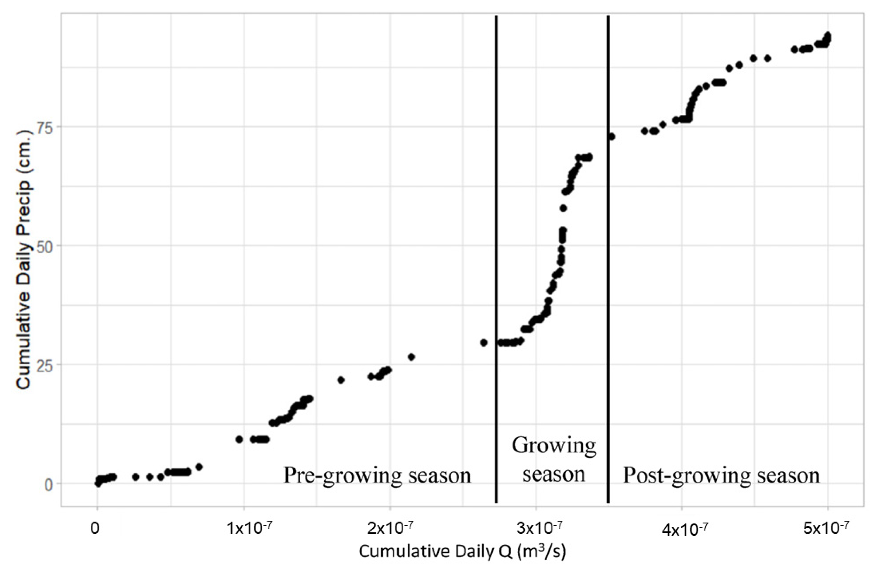
3.2. Rainfall–Runoff Variations

The discharge was largely influenced by the precipitation events during the non-growing season, namely the period before mid-May and after mid-October, as evidenced by the shift in slope seen in the double mass curve (Figure 4). During the non-growing season, the precipitation totaled 58.1 cm, with 23.8 cm of runoff (runoff is defined as the discharge volume divided by the watershed area), for a ratio of 41%. Contrary to that period, the precipitation events during the growing season from mid-May to mid-October minimally influenced the discharge, with the precipitation totaling 36.2 cm while the runoff totaled 2.3 cm for a ratio of 6%. The high-flow storm-separated data resulted in 12 storm events throughout the record period (Table 1). Finally, because the discharge was minimally impacted by the precipitation events during the growing season (Figure 4), it should be noted that there were no major discharge events during the growing season.

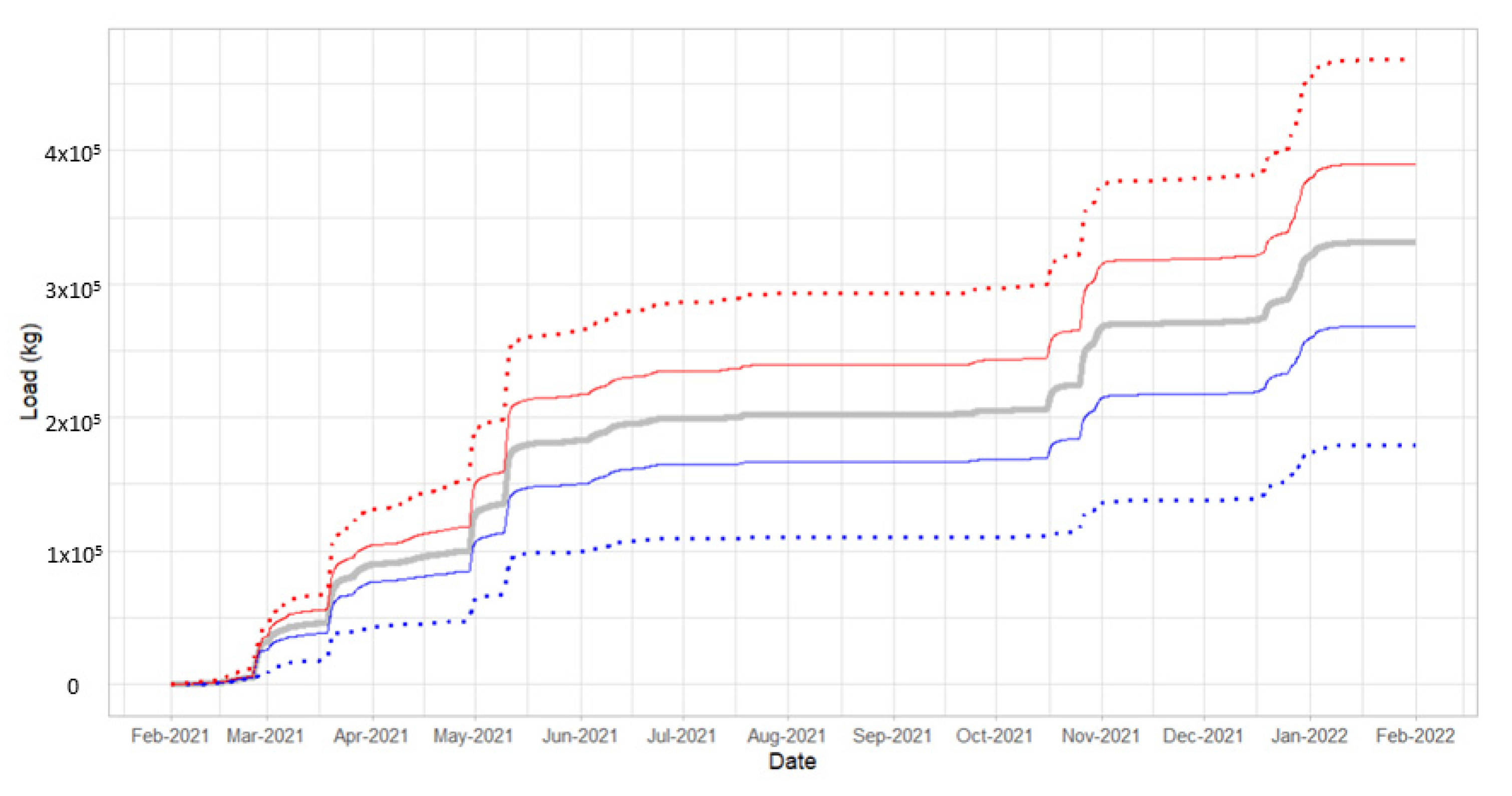
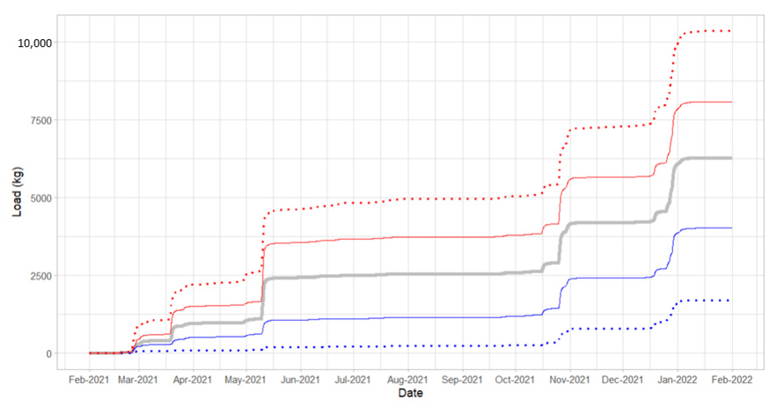
3.3. Nutrient Load Estimation

The cumulative loads were plotted for nitrate-N (Figure 5) and SRP (Figure 6). The cumulative load plots for both target nutrients had the largest increases during high-flow events. During the growing season, where the discharge remained low despite precipitation events occurring, the load minimally increased for both nutrients, regardless of the precipitation amount. Using the daily maximum and minimum concentrations to represent the range of impact under a daily sampling regime, there was an increased spread in the possible realizations of the nutrient loads across the entire sample period. The range increased the most during the high-flow events and remained rather constant for the other periods. There was an even wider spread in the realized range of the cumulative loads when considering the weekly maximum and minimum concentrations as representative samples for a given week.
Nutrient load estimations for both the daily and weekly sampling regimes and the associated percentage differences from the high-frequency “true” cumulative loads are included for nitrate-N (Table 1) and SRP (Table 2). During the growing season, the nitrate-N load percent difference from the “true” load remained around −18% for the minimum daily, +18% for the maximum daily, −46% for the minimum weekly, and +44% for the maximum weekly. During the growing season, the SRP load percent difference from the “true” load remained around −55% for the minimum daily, +47% for the maximum daily, −91% for the minimum weekly, and +94% for the maximum weekly. The annual nitrate-N load estimations from the “true” load varied by −19%, +18%, −46%, and +41% for the minimum daily, maximum daily, minimum weekly, and maximum weekly, respectively (Table 1). The annual SRP load estimations from the “true” load varied by −36%, +29%, −73%, and +65% for the minimum daily, maximum daily, minimum weekly, and maximum weekly, respectively (Table 2).

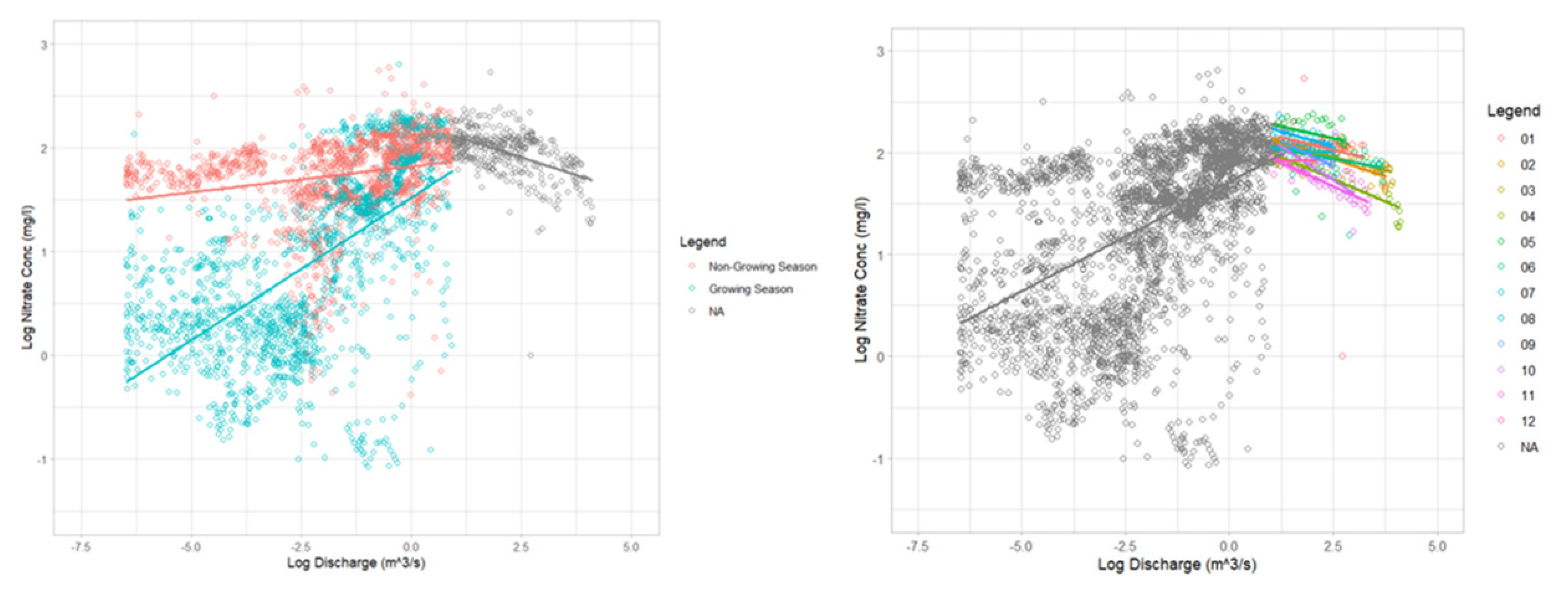
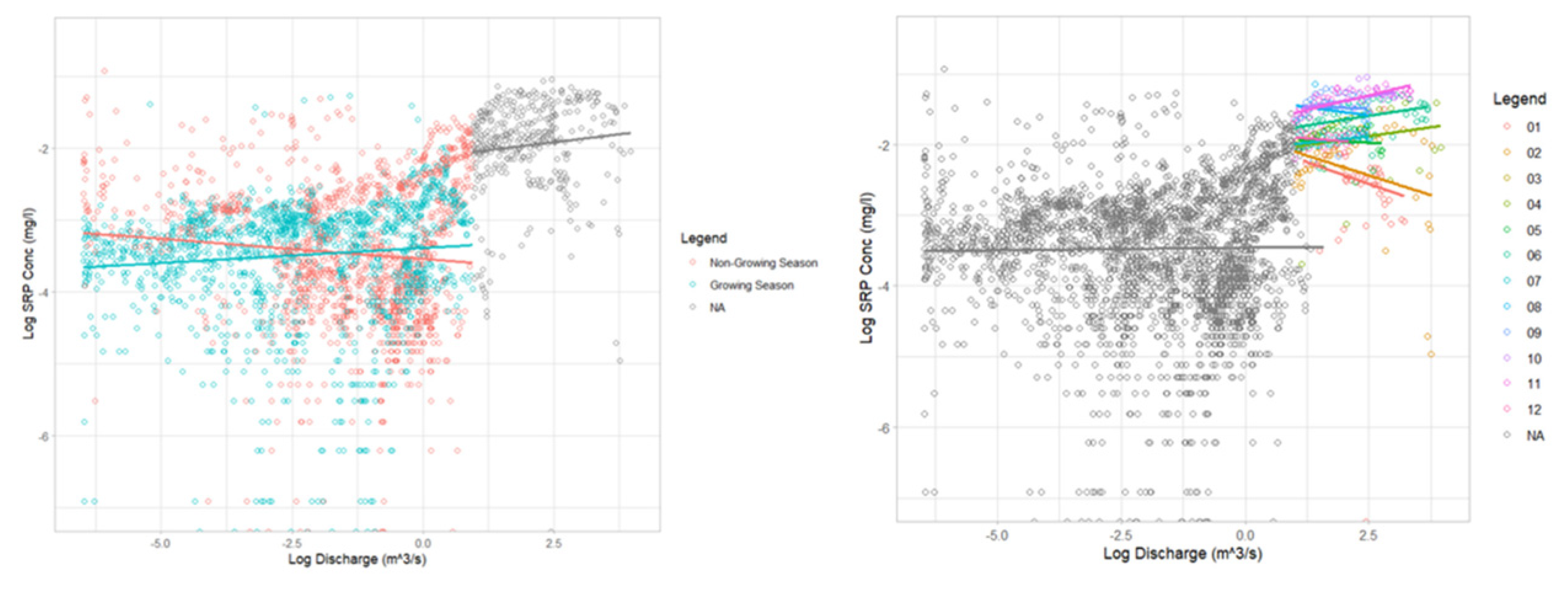
3.4. Concentration–Discharge Relations

The slopes of the nitrate-N C–Q relations during the individual storm event responses were all negative, with 7 out of the 12 events having significant negative slopes (Figure 7; Table 3). The average slope for the C–Q relations from these significant regressions, ranging from −0.07 to −0.26, was −0.16 across these seven storm events. These negative slopes indicate a dilution response of nitrate-N during storm events. Looking at the low-flow relations, we found that the nitrate-N data from the non-growing and growing seasons had significant and positive C–Q relations, indicating a mobilization response (Table 4); however, the slope for the relation was much lower for the non-growing season data (0.05) relative to the growing season data (0.27). These lower slopes indicate more chemostatic responses and an apparent shift in how nitrate-N is being loaded into downstream receiving waters. We also saw a similar shift when comparing the slopes for the lower flow conditions to those for the higher flow conditions (i.e., the individual storm events).
The slopes in the SRP C–Q relation (Figure 8) for the individual storm events exhibited greater variability than the C–Q relations from low-flow conditions (Table 3). Greater occurrences of negative C–Q slopes were observed earlier in the year (before the growing season), while more positive C–Q slopes were observed later in the year (after the growing season). The average storm event SRP C–Q slope before mid-May and at the beginning of the growing season was −0.13, while after mid-October and the end of the growing season, it was 0.04. However, only three of the linear regressions had significant slopes, and these were all positive and all occurred after the growing season during the storms between October and January. The low-flow growing and non-growing season data exhibited significant linear slopes for the regression fit to the C–Q plots, where the growing season exhibited a positive slope (0.04) and the non-growing season exhibited a negative slope (−0.06). These shifts towards apparently more chemostatic responses imply a shift in how phosphorus is being loaded into the water under lower flow conditions relative to higher flow conditions.

4. Discussion

4.1. Comparing Event-Scale and Seasonal Nutrient Responses

Considering the nutrient loads, Fink and Misch [24] found the nitrogen and phosphorus peak loading periods to occur at the beginning of the growing season (May), shortly following fertilizer applications in an agricultural, western Ohio watershed. Our cumulative load plots express a similar pattern, with a large increase in May, prior to the growing season. The annual cumulative load did not drastically increase during the growing season of the region (from mid-May to mid-October). The discharge was minimally impacted by the precipitation events during that time (Figure 4), and the cumulative load plots reflect that minimal impact. This is further evidenced by the stable percentage differences of the daily and weekly values from the “true” load during the growing season (Figure 5 and Figure 6), despite the wide load range based on the sampling frequency.
High-flow events that drive nutrient loading are not uncommon. For example, in a primarily agricultural watershed using one-hour frequency data, Liu et al. [25] calculated that 50% of the nitrate-N load was generated during only 10% of the time during high-flow events. For our site, the cumulative load plots for nitrate-N and SRP depict that the nutrient load is strongly correlated to the discharge in this watershed, confirming the studies by Basu et al. [20] and Royer et al. [26], which found that 50% and 80% of the nitrogen and phosphorus loads, respectively, occur during high-flow events.
Furthermore, for the event-scale nitrate-N responses, despite the load increases being driven by high-flow events, consistent dilution responses were identified in the high-frequency data (Figure 7). This type of event-based nitrate-N dilution response can be common in agricultural watersheds (e.g., [27]), especially after the first runoff following nutrient applications at planting. Such response differs, however, from the typical chemostatic response seen in more permeable watersheds with deep unsaturated zones and low “flashiness”. In such dampened systems, the chemostatic response has been attributed to nitrate-N accumulation in the subsurface [28,29,30]. Thus, our event-scale dilution potentially aligns more with the responses exhibited by watersheds where nitrate-N is flushed on a storm-to-storm basis [12]. As the ubiquitous tile drainage in our watershed causes “flashier” stream responses (e.g., [31]), we would anticipate shorter water residence times in the subsurface, potentially promoting event-scale dilution [32].
However, the water residence time is not the only aspect controlling the nitrate-N concentrations in the stream, as source concentrations, positions in the landscape, and soil retention are other factors to be considered. For example, looking at the low-flow responses, clear mobilization patterns were exhibited in the growing season nitrate-N C–Q relation results, and there was considerable variability in the concentrations (Figure 3). Previous efforts have attributed such mobilization of nitrate-N to water table rises and antecedent soil moisture [33,34], as nitrate-N is typically well-distributed in the soil matrix and is found in high concentrations in shallow groundwater. Other studies also suggest that the steeper positive C–Q slopes under low-flow conditions (rather than under high-flow conditions) are linked to biological nitrate-N uptake, which is often manifested as a bent rather than a linear C–Q relation [35]. This interpretation from Dehaspe et al. [35] is consistent with this current study’s C–Q relation patterns and warrants additional study, especially given the variability in the nitrate-N concentrations at low flows in this system. Further, Heathwaite and Bieroza [36] saw mobilizing responses for nitrate-N across watersheds when the concentrations considered were relatively lower than in other watersheds exhibiting chemotactic responses. As such, our observed mobilization response that emerges during the growing season conditions could be a result of relatively lower nitrate-N concentrations as water tables fall below the existing tile drainage networks in the watershed, such that deeper groundwater dominates the stream response in combination with the instream biological uptake.
Our results for SRP at the event scale (Figure 8) showed a more variable response in the C–Q relation slopes observed for the storm events and a shift from predominantly negative to predominantly positive slopes over the year. Based on our data, the SRP C–Q relations also appear to have considerable hysteresis, such that the rising limb of the hydrograph and the falling limb have different nutrient concentration responses to the changing flow (Figure 3). For the agriculturally heavy northwest Ohio region, this is somewhat expected, as sustained elevated nutrient concentrations after high-flow storm events often occur attributed to the dense tile drain network (e.g., [37]). As we transition from wetter pre-growing season conditions to dry growing season conditions, we can see the corresponding shift in the C–Q relations and the closer alignment between the peak flows and the peak concentrations (Figure 3). This represents a potential SRP transport pathway shift during the non-growing season that would be consistent with the research from the region. For example, a negative C–Q relation indicating a dilution response was seen for dissolved reactive phosphorus in combined surface and subsurface agricultural runoff in Pennsylvania [38]. Contrary to this, Osterholz et al. [39] saw in Ohio that tile drainage dissolved reactive phosphorus concentrations increased as the discharge increased, which indicates a mobilizing response. At the event scale, the C–Q patterns may, thus, ultimately be linked to soil P status, with a potential contributing influence of the flow path connectivity and the mixing of event water with the matrix and shallow groundwater as more surficial flow pathways activate under larger discharge events.
Consistent with Stamm et al. [40], such patterns of variability across events highlight that subsurface discharge water is composed of both shallow groundwater and precipitation water that has infiltrated through the soil and moved downward either by a matrix or preferential flow. Thus, the mixing of dissolved phosphorus-rich water from P-rich surface soils with P-poor groundwater could explain the variable response observed in the event-scale phosphorus C–Q responses across the year. Phosphorus-rich surface soils have been identified as the primary source of P in tile drains. Welikhe et al. [41] showed an 8-fold greater risk of dissolved reactive phosphorus loss to tile discharge for phosphorus-rich soils. In the Western Lake Erie Basin, recent work has demonstrated how the tile drainage, which is ubiquitous for the region, leads to a more direct connection between the precipitation and stream discharge, manifested as flashier stream responses [31] and a subsequent shift in the downstream phosphorus loading as a function of the system’s wetness conditions [32]. Similarly in Indiana, Williams et al. [32] saw elevated dissolved phosphorus concentrations in tile discharge coinciding with peak event water contribution from preferential flow pathways before the waters, i.e., preferential and matrix flows, mixed along the flow pathway. Taken together, the variability in the SRP C–Q relations emphasizes that nutrient losses from agricultural landscapes are driven by hydrology [42], as it intersects with the loading sources.

4.2. Implications for Management That Consider Region-Specific Conditions

Looking at the Western Lake Erie Basin, where our study watershed is located, the flat topography and extensive tile drainage networks are at greater risk for phosphorus loss as they promote the presence of dense networks of preferential flow pathways or macropores [43,44], which can allow runoff to bypass potential buffering by subsoils. Furthermore, the limited variation in topography in the region combined with clay soils has been seen as allowing for a greater potential for dissolved phosphorus losses, including colloidal forms [45]. Given these unique conditions, the application of specific conservation practices in certain environments (e.g., no-till with surface application, cover crops, etc.) may not be as effective as expected and can even lead to unintended consequences [46].
In this regard, high-temporal resolution nutrient data could help to tailor management practice recommendations to region-specific conditions. Further, high-temporal resolution monitoring over longer durations, such as the year explored in this current study, allows for variations in the dominance of hydrological and biochemical processes to be seen through shifts in the C–Q relations between relative storm events and seasons. For example, during periods of nutrient mobilization, such as the low-flow growing season nitrate-N response and the early-season storm event SRP response seen in this study, mitigation measures would need to intercept the dominant delivery pathways and target critical source areas to reduce nutrient loading [47]. These management practices could include options such as drainage water management to hold phosphorus-rich early-season runoff back in farm fields or phosphorus bioreactors that collect and process tile drainage runoff. In the case of periods with chemostatic responses, where short-term solutions can be rather ineffective, large-scale mitigation approaches will be needed [30,48], such as whole-farm management plans targeting, for example, soil health, which require a good cooperation between decision makers, farmers, and scientists [36]. Of course, it should be noted that the cost of such high-temporal resolution data (and the associated in situ wet-chemistry setup and infrastructure) often makes it cost prohibitive to have these data across many locations or spatial scales. Despite such potential limitations, pairing high-temporal resolution monitoring with more traditional synoptic or spatially distributed grab sampling could help improve the information content available, allowing for guidance on water management decisions across a watershed or a region.
Macrae et al. [46] believe that it is possible to provide a “toolkit” of general principles that can guide decision makers about conservation practice choices that may be appropriate for a given region. According to them, this would not negate the importance of individual fields, farms, and fertility management approaches in optimizing conservation practice selections, but rather guide choices with the greatest likelihood of success. Given the advances in the high-temporal frequency monitoring of nutrients, it seems that the accompanying resurgent interest in C–Q analyses could help in this optimization of the practice selection. Bieroza et al. [12] have demonstrated that the C–Q slope is a robust descriptor of the catchment’s tendency to store and transport chemicals. Furthermore, they suggest that C–Q relations can be useful to detect and characterize potential future changes (e.g., lower nitrogen or phosphorous concentrations or shifts to higher rainfall and flashiness), as these changes will manifest shifts in the C–Q responses in agricultural watersheds from chemostatic to chemodynamic (specifically mobilizing) responses.
Heathwaite and Beiroza [36] suggested that C–Q relations in combination with hydrochemical indices can be used to fingerprint the effects of hydrological disturbance on freshwater quality and can be useful in determining the impacts of global changes on stream ecology. Despite the large storm-to-storm variability in hydrochemical responses, storm event magnitude and timing have a critical role in controlling the type of mobilization, flushing, and cycling behaviors of water quality constituents. We can couple this with the recent notion that biogeochemical cycling is switched off or severely dampened depending on the magnitude of the storm event, such that higher magnitude storm events are thought to have greater damping effects [49,50] compared to lower magnitude storm events that can preserve diel cycles [51]. By combining these two concepts, we gain a basis by which we can not only characterize synergies between biogeochemical and hydrological processes, but also align sustainable management practices with mechanisms that lead to nutrient transport.

5. Concluding Remarks

The increasing availability of long-term and high-frequency datasets improves our ability to observe patterns in C–Q relations and, subsequently, advances our coupled hydrologic and biogeochemical mechanistic understanding. These high-frequency water quality data are empowering water resource managers and scientists to better understand and manage stream hydrochemistry and ecology. This monitoring technology is being incorporated into studies to better identify the mechanisms behind how and why watersheds store and release under varying conditions. New technologies that allow for similar (or even better) high-temporal frequency monitoring of nutrients, namely nitrogen and phosphorus, have the potential to be game changers, not only with regards to mechanistic understanding but also in terms of how we can better address the specific water quality problems that are being faced in watersheds. Ultimately, high-frequency temporal nutrient data monitored over long durations can guide the decisions of water resource managers and help track progress toward water quality goals.

Author Contributions

Conceptualization, S.P. and S.W.L.; methodology, S.P., J.M.H. and S.W.L.; field-work investigations, S.P. and B.M.; lab-based investigations, S.P. and B.M.; formal analysis, S.P.; writing and original draft preparation, S.P. and S.W.L.; editing and writing contributions, S.P., J.M.H., H.R., B.M. and S.W.L.; funding acquisition, H.R. and S.W.L. All authors have read and agreed to the published version of the manuscript.

Funding

This work was partially supported by the USDA National Institute of Food and Agriculture (NIFA) Agriculture and Food Research Initiative (AFRI) grant #2021-68014-34142.

Institutional Review Board Statement

Not applicable.

Informed Consent Statement

Not applicable.

Data Availability Statement

All data are available upon request.

Acknowledgments

We thank Douglas L. Moyer, U.S. Geological Survey, for the valuable feedback on an early version of this paper.

Conflicts of Interest

The authors declare no conflict of interest.

References

  1. Bieroza, M.Z.; Heathwaite, A.L. Unravelling organic matter and nutrient biogeochemistry in groundwater-fed rivers under baseflow conditions: Uncertainty in in situ high-frequency analysis. Sci. Total Environ. 2016, 572, 1520–1533. [Google Scholar] [CrossRef] [PubMed] [Green Version]
  2. Elwan, A.; Singh, R.; Patterson, M.; Roygard, J.; Horne, D.; Clothier, B.; Jones, G. Influence of sampling frequency and load calculation methods on quantification of annual river nutrient and suspended solids loads. Environ. Monit. Assess. 2018, 190, 1–18. [Google Scholar] [CrossRef] [PubMed]
  3. Birgand, F.; Appelboom, T.W.; Chescheir, G.M.; Skaggs, R.W. Estimating Nitrogen, Phosphorus, and Carbon Fluxes in Forested and Mixed-Use Watersheds of the Lower Coastal Plain of North Carolina: Uncertainties Associated with Infrequent Sampling. Trans. ASABE 2011, 54, 2099–2110. [Google Scholar] [CrossRef]
  4. Lloyd, C.E.M.; Freer, J.E.; Johnes, P.J.; Coxon, G.; Collins, A.L. Discharge and nutrient uncertainty: Implications for nutrient flux estimation in small streams: Discharge and Nutrient Uncertainty: Implications for Nutrient Fluxes. Hydrol. Process. 2016, 30, 135–152. [Google Scholar] [CrossRef] [Green Version]
  5. Lessels, J.S.; Bishop, T.F.A. A post-event stratified random sampling scheme for monitoring event-based water quality using an automatic sampler. J. Hydrol. 2020, 580, 123393. [Google Scholar] [CrossRef]
  6. Knapp, J.L.A.; von Freyberg, J.; Studer, B.; Kiewiet, L.; Kirchner, J.W. Concentration–discharge relationships vary among hydrological events, reflecting differences in event characteristics. Hydrol. Earth Syst. Sci. 2020, 24, 2561–2576. [Google Scholar] [CrossRef]
  7. Robertson, D.M.; Roerish, E.D. Influence of various water quality sampling strategies on load estimates for small streams. Water Resour. Res. 1999, 35, 3747–3759. [Google Scholar] [CrossRef]
  8. Johnes, P.J. Uncertainties in annual riverine phosphorus load estimation: Impact of load estimation methodology, sampling frequency, baseflow index and catchment population density. J. Hydrol. 2007, 332, 241–258. [Google Scholar] [CrossRef]
  9. Clement, A. Improving uncertain nutrient load estimates for Lake Balaton. Water Sci. Technol. 2001, 43, 279–286. [Google Scholar] [CrossRef]
  10. O′Grady, J.; Zhang, D.; O′Connor, N.; Regan, F. A Comprehensive Review of Catchment Water Quality Monitoring Using a Tiered Framework of Integrated Sensing Technologies. Sci. Total Environ. 2021, 765, 142766. [Google Scholar] [CrossRef]
  11. Rode, M.; Wade, A.J.; Cohen, M.J.; Hensley, R.T.; Bowes, M.J.; Kirchner, J.W.; Arhonditsis, G.B.; Jordan, P.; Kronvang, B.; Halliday, S.J.; et al. Sensors in the stream: The high-frequency wave of the present. Environ. Sci. Technol. 2016, 50, 10297–10307. [Google Scholar] [CrossRef] [PubMed] [Green Version]
  12. Bieroza, M.Z.; Heathwaite, A.L.; Bechmann, M.; Kyllmar, K.; Jordan, P. The concentration-discharge slope as a tool for water quality management. Sci. Total Environ. 2018, 630, 738–749. [Google Scholar] [CrossRef] [PubMed] [Green Version]
  13. Minaudo, C.; Dupas, R.; Gascuel-Odoux, C.; Roubeix, V.; Danis, P.A.; Moatar, F. Seasonal and event-based concentration-discharge relationships to identify catchment controls on nutrient export regimes. Adv. Water Resour. 2019, 131, 103379. [Google Scholar] [CrossRef]
  14. Welikhe, P.; Brouder, S.M.; Volenec, J.J.; Gitau, M.; Turco, R.F. Dynamics of dissolved reactive phosphorus loss from phosphorus source and sink soils in tile-drained systems. J. Soil Water Conserv. 2022, 77, 1–14. [Google Scholar] [CrossRef]
  15. Floury, P.; Gaillardet, J.; Gayer, E.; Bouchez, J.; Tallec, G.; Ansart, P.; Koch, F.; Gorge, C.; Blanchouin, A.; Roubaty, J.-L. The potamochemical symphony: New progress in the high-frequency acquisition of stream chemical data. Hydrol. Earth Syst. Sci. 2017, 21, 6153–6165. [Google Scholar] [CrossRef] [Green Version]
  16. Jordan, P.; Melland, A.R.; Mellander, P.E.; Shortle, G.; Wall, D. The seasonality of phosphorus transfers from land to water: Implications for trophic impacts and policy evaluation. Sci. Total Environ. 2012, 434, 101–109. [Google Scholar] [CrossRef]
  17. Muenich, R.L.; Kalcic, M.; Scavia, D. Evaluating the Impact of Legacy P and Agricultural Conservation Practices on Nutrient Loads from the Maumee River Watershed. Environ. Sci. Technol. 2016, 50, 8146–8154. [Google Scholar] [CrossRef]
  18. Lake Erie Commission. Promoting Clean and Safe Water in Lake Erie: Ohio’s Domestic Action Plan 2020 to Address Nutrients. 2020. Available online: https://lakeerie.ohio.gov/planning-and-priorities/02-domestic-action-plan (accessed on 21 July 2022).
  19. CoCoRaHS-Community Collaborative Rain, Hail & Snow Network. 2022. Available online: https://www.cocorahs.org/ViewData/ListDailyPrecipReports.aspx (accessed on 21 July 2022).
  20. Basu, N.B.; Destouni, G.; Jawitz, J.W.; Thompson, S.E.; Loukinova, N.V.; Darracq, A.; Zanardo, S.; Yaeger, M.; Sivapalan, M.; Rinaldo, A.; et al. Nutrient loads exported from managed catchments reveal emergent biogeochemical stationarity. Geophys. Res. Lett. 2010, 37. [Google Scholar] [CrossRef]
  21. Godsey, S.E.; Kirchner, J.W.; Clow, D.W. Concentration-discharge relationships reflect chemostatic characteristics of US catchments. Hydrol. Process. 2009, 23, 1844–1864. [Google Scholar] [CrossRef] [Green Version]
  22. Minaudo, C.; Dupas, R.; Gascuel-Odoux, C.; Fovet, O.; Mellander, P.-E.; Jordan, P.; Shore, M.; Moatar, F. Nonlinear empirical modeling to estimate phosphorus exports using continuous records of turbidity and discharge. Water Resour. Res. 2017, 53, 7590–7606. [Google Scholar] [CrossRef]
  23. R Core Team. R: A Language and Environment for Statistical Computing. Vienna, Austria: R Foundation for Statistical Computing. 2017. Available online: https://www.r-project.org/ (accessed on 21 July 2022).
  24. Fink, D.F.; Mitsch, W.J. Seasonal and storm event nutrient removal by a created wetland in an agricultural watershed. Ecol. Eng. 2004, 23, 313–325. [Google Scholar] [CrossRef]
  25. Liu, W.; Youssef, M.A.; Birgand, F.P.; Chescheir, G.M.; Tian, S.; Maxwell, B.M. Processes and mechanisms controlling nitrate dynamics in an artificially drained field: Insights from high-frequency water quality measurements. Agric. Water Manag. 2020, 232, 106032. [Google Scholar] [CrossRef]
  26. Royer, T.V.; David, M.B.; Gentry, L.E. Timing of Riverine Export of Nitrate and Phosphorus from Agricultural Watersheds in Illinois: Implications for Reducing Nutrient Loading to the Mississippi River. Environ. Sci. Technol. 2006, 40, 4126–4131. [Google Scholar] [CrossRef] [PubMed]
  27. Bowes, M.J.; Jarvie, H.P.; Halliday, S.J.; Skeffington, R.A.; Wade, A.J.; Loewenthal, M.; Gozzard, E.; Newman, J.R.; Palmer-Felgate, E.J. Characterising phosphorus and nitrate inputs to a rural river using high-frequency concentration-flow relationships. Sci. Total Environ. 2015, 511, 608–620. [Google Scholar] [CrossRef] [PubMed] [Green Version]
  28. Ascott, M.J.; Wang, L.; Stuart, M.E.; Ward, R.S.; Hart, A. Quantification of nitrate storage in the vadose (unsaturated) zone: A missing component of terrestrial N budgets. Hydrol. Process. 2016, 30, 1903–1915. [Google Scholar] [CrossRef] [Green Version]
  29. Howden, N.J.K.; Burt, T.P.; Worrall, F.; Whelan, M.J.; Bieroza, M. Nitrate concentrations and fluxes in the river Thames over 140 years (1868–2008): Are increases irreversible? Hydrol. Process. 2010, 24, 2657–2662. [Google Scholar] [CrossRef]
  30. Van Meter, K.J.; Basu, N.B.; Van Cappellen, P. Two centuries of nitrogen dynamics: Legacy sources and sinks in the Mississippi and Susquehanna River basins. Glob. Biogeochem. Cycles 2017, 31, 2–23. [Google Scholar] [CrossRef] [Green Version]
  31. Miller, S.A.; Lyon, S.W. Tile drainage causes flashy streamflow response in Ohio watersheds. Hydrol. Process. 2021, 35, e14326. [Google Scholar] [CrossRef]
  32. Williams, M.R.; King, K.W.; Ford, W.; Fausey, N.R. Edge-of-field research to quantify the impacts of agricultural practices on water quality in Ohio. J. Soil Water Conserv. 2016, 71, 9A–12A. [Google Scholar] [CrossRef] [Green Version]
  33. Macrae, M.L.; English, M.C.; Schiff, S.L.; Stone, M. Influence of antecedent hydrologic conditions on patterns of hydrochemical export from a first-order agricultural watershed in Southern Ontario, Canada. J. Hydrol. 2010, 389, 101–110. [Google Scholar] [CrossRef]
  34. Wagner, L.E.; Vidon, P.; Tedesco, L.P.; Gray, M. Stream nitrate and DOC dynamics during three spring storms across land uses in glaciated landscapes of the Midwest. J. Hydrol. 2008, 362, 177–190. [Google Scholar] [CrossRef]
  35. Dehaspe, J.; Sarrazin, F.; Kumar, R.; Fleckenstein, J.H.; Musolff, A. Bending of the concentration discharge relationship can inform about in-stream nitrate removal. Hydrol. Earth Syst. Sci. 2021, 25, 6437–6463. [Google Scholar] [CrossRef]
  36. Heathwaite, A.L.; Bieroza, M. Fingerprinting hydrological and biogeochemical drivers of freshwater quality. Hydrol. Process. 2021, 35, e13973. [Google Scholar] [CrossRef]
  37. Miller, S.A.; Lyon, S.W. Tile drainage increases runoff and phosphorus export during wet years in the Western Lake Erie Basin. Front. Water 2021, 3, 757106. [Google Scholar] [CrossRef]
  38. Miller, M.D.; Gall, H.E.; Buda, A.R.; Saporito, L.S.; Veith, T.L.; White, C.M.; Williams, C.F.; Brasier, K.J.; Kleinman, P.J.A.; Watson, J.E. Load-discharge relationships reveal the efficacy of manure application practices on phosphorus and total solids losses from agricultural fields. Agric. Ecosyst. Environ. 2019, 272, 19–28. [Google Scholar] [CrossRef]
  39. Osterholz, W.R.; Hanrahan, B.R.; King, K.W. Legacy phosphorus concentration–discharge relationships in surface runoff and tile drainage from Ohio crop fields. J. Environ. Qual. 2020, 49, 675–687. [Google Scholar] [CrossRef]
  40. Stamm, C.; Flühler, H.; Gächter, R.; Leuenberger, J.; Wunderli, H. Preferential transport of phosphorus in drained grassland soils. J. Environ. Qual. 1998, 27, 515–522. [Google Scholar] [CrossRef]
  41. Welikhe, P.; Brouder, S.M.; Volenec, J.J.; Gitau, M.; Turco, R.F. Development of phosphorus sorption capacity-based environmental indices for tile-drained systems. J. Environ. Qual. 2020, 49, 378–391. [Google Scholar] [CrossRef]
  42. Williams, M.R.; Buda, A.R.; Elliott, H.A.; Hamlett, J.; Boyer, E.W.; Schmidt, J.P. Groundwater flow path dynamics and nitrogen transport potential in the riparian zone of an agricultural headwater catchment. J. Hydrol. 2014, 511, 870–879. [Google Scholar] [CrossRef]
  43. King, K.W.; Williams, M.R.; Fausey, N.R. Contributions of systematic tile drainage to watershed-scale phosphorus transport. J. Environ. Qual. 2015, 44, 486–494. [Google Scholar] [CrossRef] [Green Version]
  44. Simard, R.R.; Beauchemin, S.; Haygarth, P.M. Potential for preferential pathways of phosphorus transport. J. Environ. Qual. 2000, 29, 97–105. [Google Scholar] [CrossRef]
  45. River, M.; Richardson, C.J. Dissolved reactive phosphorus loads to western Lake Erie: The hidden influence of nanoparticles. J. Environ. Qual. 2019, 48, 645–653. [Google Scholar] [CrossRef] [Green Version]
  46. Macrae, M.; Jarvie, H.; Brouwer, R.; Gunn, G.; Reid, K.; Joosse, P.; King, K.; Kleinman, P.; Smith, D.; Williams, M.; et al. One size does not fit all: Toward regional conservation practice guidance to reduce phosphorus loss risk in the Lake Erie watershed. J. Environ. Qual. 2021, 50, 529–546. [Google Scholar] [CrossRef]
  47. Harris, G.P.; Heathwaite, A.L. Why is achieving good ecological outcomes in rivers so difficult? Freshw. Biol. 2012, 57, 91–107. [Google Scholar] [CrossRef]
  48. Ockenden, M.C.; Hollaway, M.J.; Beven, K.J.; Collins, A.L.; Evans, R.; Falloon, P.D.; Forber, K.J.; Hiscock, K.M.; Kahana, R.; Macleod, C.J.A.; et al. Major agricultural changes required to mitigate phosphorus losses under climate change. Nat. Commun. 2017, 8, 161. [Google Scholar] [CrossRef] [Green Version]
  49. Bernhardt, E.S.; Heffernan, J.B.; Grimm, N.B.; Stanley, E.H.; Harvey, J.W.; Arroita, M.; Appling, A.P.; Cohen, M.J.; McDowell, W.H.; Hall, R.O., Jr.; et al. The metabolic regimes of flowing waters. Limnol. Oceanogr. 2018, 63, S99–S118. [Google Scholar] [CrossRef] [Green Version]
  50. Raymond, P.A.; Saiers, J.E.; Sobczak, W.V. Hydrological and biogeochemical controls on watershed dissolved organic matter transport: Pulse-shunt concept. Ecology 2016, 97, 5–16. [Google Scholar] [CrossRef] [Green Version]
  51. Burns, D.A.; Pellerin, B.A.; Miller, M.P.; Capel, P.D.; Tesoriero, A.J.; Duncan, J.M. Monitoring the riverine pulse: Applying high-frequency nitrate data to advance integrative understanding of biogeochemical and hydrological processes. Wiley Interdiscip. Rev. Water 2019, 6, e1348. [Google Scholar] [CrossRef]
Figure 1. Site map of the Little Auglaize River watershed, located in northwestern Ohio, with the flyout image showing the monitored intake where the Greeneyes NuLab autonomous nutrient analyzer (NuLab) was sampling water and the streamflow was measured.
Sustainability 14 16848 g001
Figure 2. Major elements of the Greeneyes NuLab autonomous nutrient analyzer (NuLab), installed at the water intake for the Delphos Gillmor reservoir along the Little Auglaize River in northwestern Ohio.
Sustainability 14 16848 g002
Figure 3. Timeseries of nitrate-N and SRP concentrations, discharge (Q), and precipitation for the study period. The gray bars indicate regions where nutrient data were not available from the 2-h sampling using the NuLab.
Sustainability 14 16848 g003
Figure 4. Double mass curve of cumulative daily precipitation against cumulative daily streamflow, with the vertical lines indicating the beginning (mid-May) and the end (mid-October) of the growing season.
Sustainability 14 16848 g004
Figure 5. Cumulative load plot for nitrate-N of the high-frequency “true” load (gray), the daily maximum and minimum cumulative load estimations (red and blue solid lines), and the weekly maximum and minimum cumulative load estimations (red and blue dotted lines); all of the nutrient loads were calculated with a two-hour discharge.
Sustainability 14 16848 g005
Figure 6. Cumulative load plot for SRP of the high-frequency “true” load (gray), the daily maximum and minimum cumulative load estimations (red and blue solid lines), and the weekly maximum and minimum cumulative load estimations (red and blue dotted lines); all of the nutrient loads were calculated with a two-hour discharge.
Sustainability 14 16848 g006
Figure 7. Concentration–discharge (C–Q) relations for the high-frequency nitrate-N data, showing a linear regression fit for the low-flow conditions over the growing and non-growing seasons (left panel) and the individual event-based responses (right panel). The event numbers correspond to those listed in Table 1.
Sustainability 14 16848 g007
Figure 8. Concentration–discharge (C–Q) relations for the high-frequency SRP data, showing a linear regression fit for the low-flow conditions over the growing and non-growing seasons (left panel) and the individual event-based responses (right panel). The event numbers correspond to those listed in Table 1.
Sustainability 14 16848 g008
Table 1. Percentage difference for the cumulative load estimations from the high-frequency “true” cumulative load for nitrate-N.
Cumulative Load (kg)Percent Difference Using Daily ConcentrationsPercent Difference Using Weekly Concentrations
MonthHigh-FrequencyMin DailyMax DailyMin WeeklyMax WeeklyMinMaxMinMax
February31,34525,59134,852753141,331−18%11%−76%32%
March90,23076,980104,63642,821131,122−15%16%−53%45%
April126,893106,065149,78763,023188,851−16%18%−50%49%
May183,203150,437217,42099,203265,578−18%19%−46%45%
June199,377164,965235,143109,094286,114−17%18%−45%44%
July202,664167,050239,746110,152292,771−18%18%−46%44%
August202,768167,126239,890110,215293,037−18%18%−46%45%
September205,531168,773243,228110,471297,212−18%18%−46%45%
October267,894214,799315,208135,296373,771−20%18%−49%40%
November271,450217,640319,429137,974379,100−20%18%−49%40%
December321,202259,566379,250173,440454,041−19%18%−46%41%
January331,640268,889390,484179,521468,188−19%18%−46%41%
Table 2. Percentage difference for the cumulative load estimations from the high-frequency “true” cumulative load for SRP.
Cumulative Load (kg) Percent Difference Using Daily Concentrations Percent Difference Using Weekly Concentrations
MonthHigh-Frequency Min DailyMax DailyMin WeeklyMax WeeklyMinMaxMinMax
February28521743256819−24%51%−80%187%
March9655161512902205−46%57%−91%129%
April10425561599962524−47%54%−91%142%
May2428106535581934632−56%47%−92%91%
June2492111236662094822−55%47%−92%93%
July2542115237322304948−55%47%−91%95%
August2544115337362304955−55%47%−91%95%
September2588118737912515031−54%46%−90%94%
October4153237855827597151−43%34%−82%72%
November4202241856597907275−42%35%−81%73%
December60743857783616009935−36%29%−74%64%
January 627140188073170310,349−36%29%−73%65%
Table 3. Individual events used to characterize the event-based concentration–discharge (C–Q) relations for both nitrate-N and SRP. The bold indicates significance, with a p-value of <0.01.
EventDatePrecip. (mm)Runoff (mm) Nitrate-NSRP
InterceptSlopeStd. Err.R2np-ValueInterceptSlopeStd. Err.R2np-Value
1Feb 24–Mar 039.120.62.28−0.100.340.02440.3461−1.90−0.300.740.04490.1594
2Mar 18–Mar 2267.127.42.29−0.140.080.7341<0.0001−1.87−0.220.690.09380.0635
3Apr 29–May 0145.723.62.22−0.100.080.6131<0.0001n/an/an/an/an/an/a
4May 09–May 1258.440.52.18−0.170.110.7735<0.0001−2.190.140.450.11360.0490
5Oct 15–Oct 1726.47.92.38−0.090.240.05250.2988−1.91−0.030.220.00250.7563
6Oct 25–Oct 2853.122.42.12−0.070.150.19360.0083−1.860.110.200.20380.0048
7Oct 29–Nov 0126.48.92.08−0.030.050.07330.1257−2.070.080.050.33330.0005
8Dec 18–Dec 2020.15.62.35−0.120.100.27200.0180−1.34−0.100.140.10210.1521
9Dec 25–Dec 2737.65.42.36−0.200.070.6119<0.0001−1.45−0.010.320.00190.9388
10Dec 27–Dec 2813.78.02.39−0.260.180.44180.0026−1.600.110.140.20170.0700
11Dec 28–Jan 0121.615.52.13−0.180.070.8139<0.0001−1.720.170.150.4542<0.0001
12Jan 02–Jan 039.43.01.94−0.010.060.00150.9031−1.84−0.060.100.05150.4306
Table 4. Linear regressions characterizing the low-flow growing and non-growing season concentration–discharge (C–Q) relations for both nitrate-N and SRP. The bold indicates significance, with a p-value of <0.01.
Nitrate-NSRP
InterceptSlopeStd. Err.R2np-ValueInterceptSlopeStd. Err.R2np-Value
Non-growing season1.820.050.360.081924<0.0001−3.050.181.060.111741<0.0001
Growing season1.530.280.670.391677<0.0001−3.430.040.840.0114530.0008
Publisher’s Note: MDPI stays neutral with regard to jurisdictional claims in published maps and institutional affiliations.

