
Effects of Weather on Iowa Nitrogen Export Estimated by Simulation-Based Decomposition

1
Department of Aerospace Eng., Iowa State University, Ames, IA 50011, USA
2
School of Aeronautics and Astronautics, Purdue University, West Lafayette, IN 47907, USA
3
Department of Agricultural and Biosystems Eng., Iowa State University, Ames, IA 50011, USA
*
Author to whom correspondence should be addressed.
Sustainability 2022, 14(3), 1060; https://0-doi-org.brum.beds.ac.uk/10.3390/su14031060
Submission received: 11 December 2021
/
Revised: 6 January 2022
/
Accepted: 8 January 2022
/
Published: 18 January 2022
(This article belongs to the Special Issue Sustainability Analysis and Environmental Decision-Making Using Simulation, Optimization, and Computational Analytics)
Abstract
:The state of Iowa is known for its high-yield agriculture, supporting rising demands for food and fuel production. But this productivity is also a significant contributor of nitrogen loading to the Mississippi River basin causing the hypoxic zone in the Gulf of Mexico. The delivery of nutrients, especially nitrogen, from the upper Mississippi River basin, is a function, not only of agricultural activity, but also of hydrology. Thus, it is important to consider extreme weather conditions, such as drought and flooding, and understand the effects of weather variability on Iowa’s food-energy-water (IFEW) system and nitrogen loading to the Mississippi River from Iowa. In this work, the simulation decomposition approach is implemented using the extended IFEW model with a crop-weather model to better understand the cause-and-effect relationships of weather parameters on the nitrogen export from the state of Iowa. July temperature and precipitation are used as varying input weather parameters with normal and log normal distributions, respectively, and subdivided to generate regular and dry weather conditions. It is observed that most variation in the soil nitrogen surplus lies in the regular condition, while the dry condition produces the highest soil nitrogen surplus for the state of Iowa.
1. Introduction
Nutrients, such as nitrogen (N), are necessary in farming for raising crop and forage productivity, but they can also bring potential harm to the socioeconomic system. A hypoxic zone is a phenomenon where low dissolved oxygen (hypoxia) occurs in aquatic environments, which is primarily caused by excess nutrients running off or leaching from the contributing watershed. Over 400 hypoxic zones have been found in the world and the problem of hypoxia is worsening [1]. In the US, the environment and socioeconomic system of the Gulf of Mexico are impacted by hypoxia which has one of the largest hypoxic zones in the world [2]. Nitrogen (N) is one of the major contributors to the creation of the hypoxic zone of the Gulf of Mexico through the nitrates (NO3) lost from watersheds within the Mississippi River Basin, which moves downstream to the Gulf of Mexico [3]. Studies show that the state of Iowa, one of the major producers of corn, soybean, ethanol, and animal products, contributes a considerable amount of nitrogen loads to the Mississippi River basin [4,5]. As the largest producer of corn in the US, nearly 57% of Iowa’s corn is used for ethanol production [6]. The manure produced by animal agriculture is also rich in nitrogen [7]. The current research aims at creating strategies and policies to mitigate the excess nitrogen originating from the Iowa food-energy-water (IFEW) system.
Climate variability has major effects on FEW systems. For example, extreme events, such as floods or droughts, can reduce water availability and quality. In southern East Africa, infrastructure design is challenging due to multi-year drought [8]. Furthermore, changes in the weather impact energy usage and demands of human activities. Moreover, in the food system, the needs for livestock watering and crop fertilizer can be severely impacted due to climates changes. Though Iowa uses primarily rain-fed agricultural production, in other areas irrigation water for crops is also significantly impacted (both in supply and in requirements) by weather and climate. Arizona is a predominantly irrigated agriculture state and supplies food to at least six major cities. It is especially vulnerable to climate changes [9]. Therefore, it is important to investigate the effects of weather variability on the sustainable management of FEW systems.
It is important to capture the complex interactions of the different domains to determine the exported nitrogen of the system. In this work, weather, water, agriculture, animal agriculture, and energy are considered in modeling the IFEW system. The macro-level simulation-based IFEW model introduced in [10] to determine the surplus nitrogen in the state of Iowa is extended to include a crop-weather model using linear regression of historical weather parameters, which is based on a prior study [11]. Simulation decomposition (SD) [12,13] is used to visualize the effects of weather variability on the IFEW nitrogen export. Furthermore, SD analysis is used to distinguish the influences of different weather scenarios affecting the surplus nitrogen.
The next section gives the details of the IFEW system model and the SD analysis technique. The following section presents the numerical results of SD applied to the proposed IFEW simulation model for several weather scenarios. The last section summarizes the work and discusses potential future work.
2. Methods
This section gives a high-level description of the IFEW system model interdependencies. The macro-level simulation-based model of the IFEW system and the SD technique are described.
2.1. IFEW System Model Interdependencies
The IFEW system model has five distinct macro-level domains, namely, weather, water, agriculture, animal agriculture, and energy (Figure 1). The weather discipline provides environmental factors, such as vapor pressure, temperature, rainfall, and solar radiation. Rainfall and snowfall supply surface water and groundwater components for the water discipline. The amount of crop production in the agriculture discipline is strongly related to precipitation and temperature [11]. The water discipline supplies water for drinking and service usage for the animal agriculture discipline, and the production and ethanol and fertilizer for the energy system. Dry distillers’ grain soluble (DDGS) that is produced during the ethanol production process and commercial fertilizers provide protein to animals and fertility to soil in the animal agriculture and agricultural domains, respectively. Demand for food protein by society is satisfied by the animal agriculture discipline. Corn yield in the agricultural discipline is used for ethanol production in the energy discipline and the satisfaction of socioeconomic demand. Other socioeconomic demands are satisfied by the corresponding domains except the weather discipline. The excess nitrogen from animal lands and crop fields is carried by water flow in the form of nitrates draining into the Mississippi River basin and further into the Gulf of Mexico.
2.2. IFEW Macro-Level Simulation Model
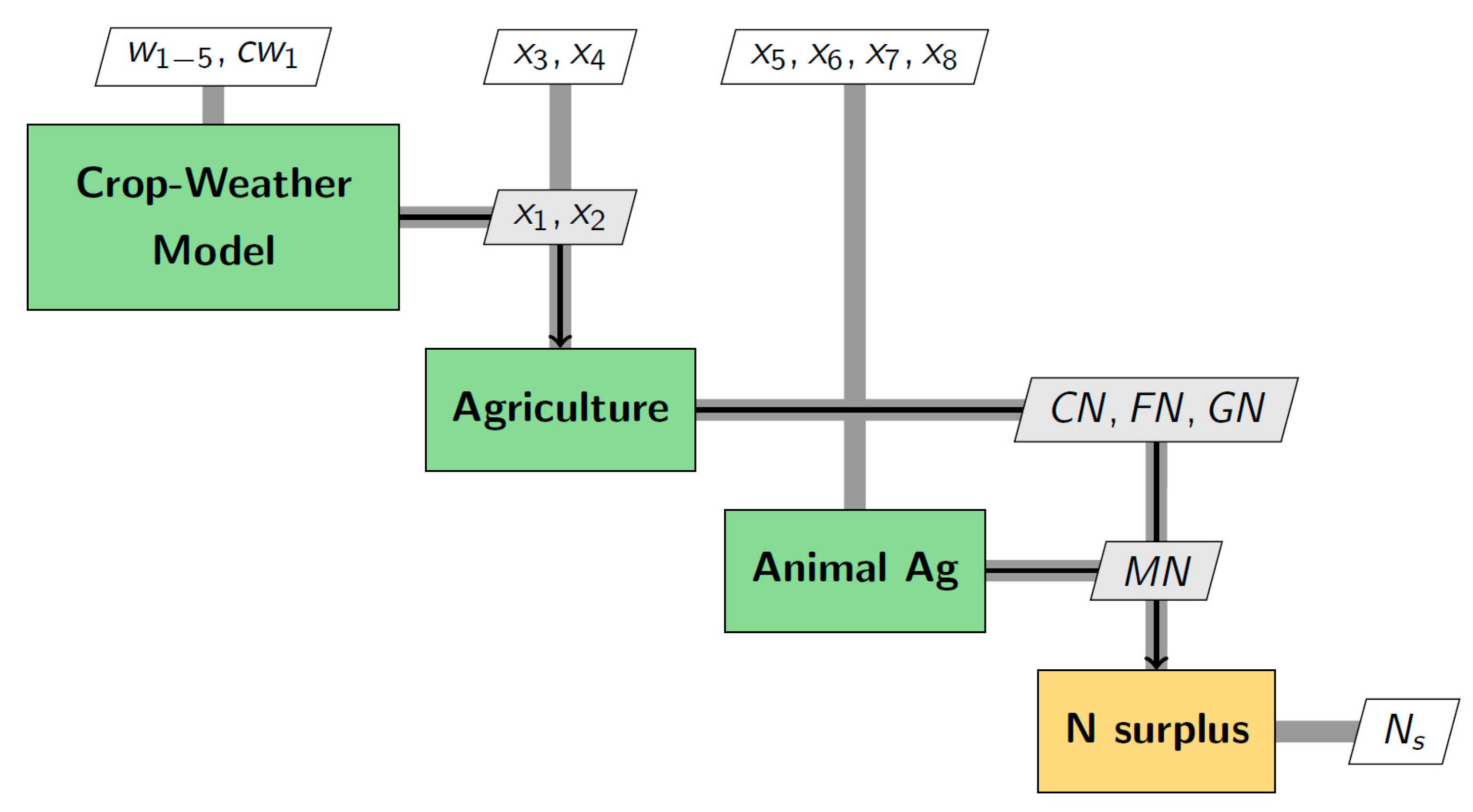
In this work, an extended simulation-based model of the IFEW system introduced in [10] is proposed to calculate the surplus nitrogen (Ns) considering only the weather, agriculture, and animal agriculture domains in Figure 1. Figure 2 shows the flow of components and the process of calculation via an extended design structure matrix (XDSM) diagram [14]. The input parameters are the weather model parameters (w1–5), May crop planting progress (cw1), rate of commercial nitrogen for corn (x3), rate of commercial nitrogen for soybean (x4), the total hog/pig population (x5), number of beef cows (x6), number of milk cows (x7), and number of other cattle (x8) including the population of steers, heifers, and slaughter cattle. Other intermediate response parameters are corn yield (x1), soybean yield (x2), the application of commercial nitrogen (CN), nitrogen generated from manure (MN), nitrogen fixed by soybean crop (FN), and the nitrogen present in harvested grain (GN). The model estimates the nitrogen surplus (Ns) based on output quantities yielded by each discipline.
This simulation model is an extension from the authors’ previous work with the addition of the crop-weather model [10]. Westcott and Jewison [11] discovered that the amount of corn yield is linear to mid-May planting progress, July temperature, and June precipitation short fall, but is nonlinear to July precipitation. Meanwhile, the productivity of soybean is linear to the average value of July and August temperatures, and June precipitation short fall, but is nonlinear to the average value of July and August precipitations. The crop-weather model of the work is developed based on [11] given a set of temperature and precipitation data of certain months over a 10-year period (2009–2019) from [15]: July temperature (w1), July precipitation (w2), June precipitation (w3), July-August average temperature (w4), and July-August average precipitation (w5). The corn yield (x1) is estimated by a regression model with May planting progress (cw1), July temperature (w1), July precipitation (w2), and June precipitation (w3). Similar to the corn model, the model for soybean yield (x2) is created using June precipitation (w3), July-August average temperature (w4), and July-August average precipitation (w5). For simplicity, July and August average values are represented by July values in this work.
The nitrogen present in harvested grain (GN) is calculated using two input parameters, namely, the corn yield (x1) and soybean yield (x2) as
where Acorn and Asoy represent the Iowa corn and the soybean acreage, whereas A represents the total area under corn and soybean crop. It is assumed that 6.4% and 1.18% of nitrogen are in the soybean seed and the corn seed while harvesting, respectively [16]. The biological nitrogen fixation from the soybean crop (FN) is estimated as [17].
The commercial nitrogen (CN) is estimated using the rate of commercial nitrogen for corn (x3) and the rate of commercial nitrogen for soybean (x4) as
The values of the corn and soybean acreages are obtained from the USDA [18]. The annual manure nitrogen contribution of each animal type is estimated [19]
where P, AMN, and LF are the livestock group population, nitrogen in animal manure, and life cycle of animal, respectively. P is substituted by the corresponding parameters with respect to different animal alternatives: the total hog/pig population (x5), number of beef cows (x6), number of milk cows (x7), and number of other cattle (x8). The total nitrogen generated from manure (MN) can be determined by the normalized sum of MN for each livestock group with total area A as
2.3. Simulation Decomposition
The simulation decomposition (SD) [12] approach is an extension to the Monte Carlo simulation [21] that enhances the explanatory capability of the simulation results by exploiting the inherent cause-and-effect relationship between the input and output parameters [13].
SD has recently been developed and successfully used on problems involved in different domains such as geology, business, and environmental science [22]. It has been shown to provide a deeper understanding of the interaction between different sources of uncertainties and its impact on output uncertainty and its distribution to stakeholders. The current section provides a brief description of SD from an application point of view. A detailed description of SD can be found in [12].
In this section, the fundamental steps of implementing SD are described using an analytical model problem. Consider a simple analytical function given as
where and are the real numbered input parameters and the real number output parameter. The SD process has the following steps [12]:
- Identify the input parameters () and their corresponding distribution ranges in which these parameters are expected to vary. Table 2 provide input parameters and their corresponding distributions. For this example, a uniform distribution is assumed for each parameter.
- Next, for each parameter the states are identified. The states of each input parameter represent a category of outcomes (e.g., low, or high). Based on the state for each parameter, a value range is determined as seen in Table 2 for the example problem.
- Generate every possible combination of the parameter states. Each combination of states represents a unique scenario () of the to-be-decomposed simulation of the output. The number of scenarios depends on the number of states of each parameter. For the example problem, the number of scenarios is four, as shown in Table 3.
- Run the Monte Carlo simulations by randomly sampling the parameters, identifying parameter states, and evaluating output. Register output of each simulated iteration for producing full output distribution and simultaneously group the output based on the scenarios for producing decomposed sub-distribution for each scenario.
- Finally, construct appropriate output graphs or tables to better understand the cause-and-effect relationship between input and output parameters. In particular, the stacked histogram is an informative graph that displays the full output distribution and the decomposed output superimposed on full distribution. Figure 3 shows the full and decomposed distribution of the simulated output.
3. Results
This section presents the results of applying SD to the proposed extended nitrogen export model which includes a weather model. In particular, the current work focuses on understanding the effects of weather parameters on the nitrogen surplus in different scenarios.
For this study, the weather parameters temperature (T) and precipitation (PPT) for July are taken as input parameters, whereas soil nitrogen surplus is considered as an output parameter computed from the IFEW simulation model. Furthermore, the July temperature is assumed to be normally distributed with a mean of 74 °F and a standard deviation of 2 °F, whereas the July precipitation is assumed to have a lognormal distribution with a standard deviation of 0.4 in., a shape parameter of 0, and median at 4 as shown in Table 4. All other parameters considered in the IFEW simulation model are kept constant.
In the crop-weather model, May plantation progress and June precipitation is assumed to be 80% and 5.5 in., respectively. The parameters used in the animal agriculture model (x5–8) are based on the 2012 Iowa animal population data [19]. The commercial nitrogen application rate for corn (x3) and soybean (x4) agriculture are considered to be constant and set as 185 kg/ha and 17 kg/ha based on the Iowa State University extension guidelines for the nitrogen application rate for corn [23] and on the fertilizer use and price data [24].
After setting up the IFEW model, Monte Carlo simulations are performed using Latin hypercube sampling (LHS) [25]. The LHS sampling method ensures that the input parameter ranges are represented appropriately. The input parameter states and boundary details are presented in Table 4. For July temperature, any temperature above 76 °F is considered to be under state high where all other temperature values are considered to be under state regular. Similarly, for July precipitation, any precipitation value below 2.5 in. is labeled under state low precipitation and all other values are under state regular. Table 5 presents the scenarios based on a combination of states. The parameter states are selected to produce some of the extreme condition scenarios (e.g., Table 5 dry condition).
A total 105 samples of input weather parameters (w1 and w2) are generated using LHS and SD approach is implemented using the IFEW simulation model. Figure 4 shows the distribution of sampled weather parameters in two states and four scenarios as mentioned in Table 4 and Table 5. Most of the generated samples are observed under regular condition (Sc2) whereas the least number of samples are observed in dry condition (Sc3).
The input weather parameters are supplied to a crop-weather module which computes corn yield (x1) and soybean yield (x2). The computed crop yield values are then passed to an agriculture module where CN, FN, and GN values are computed as mentioned in Section 2.2. Here, the contribution of CN will be constant for every IFEW model evaluation due to the assumption of a constant commercial nitrogen application rate for corn (x3) and soybean (x4).
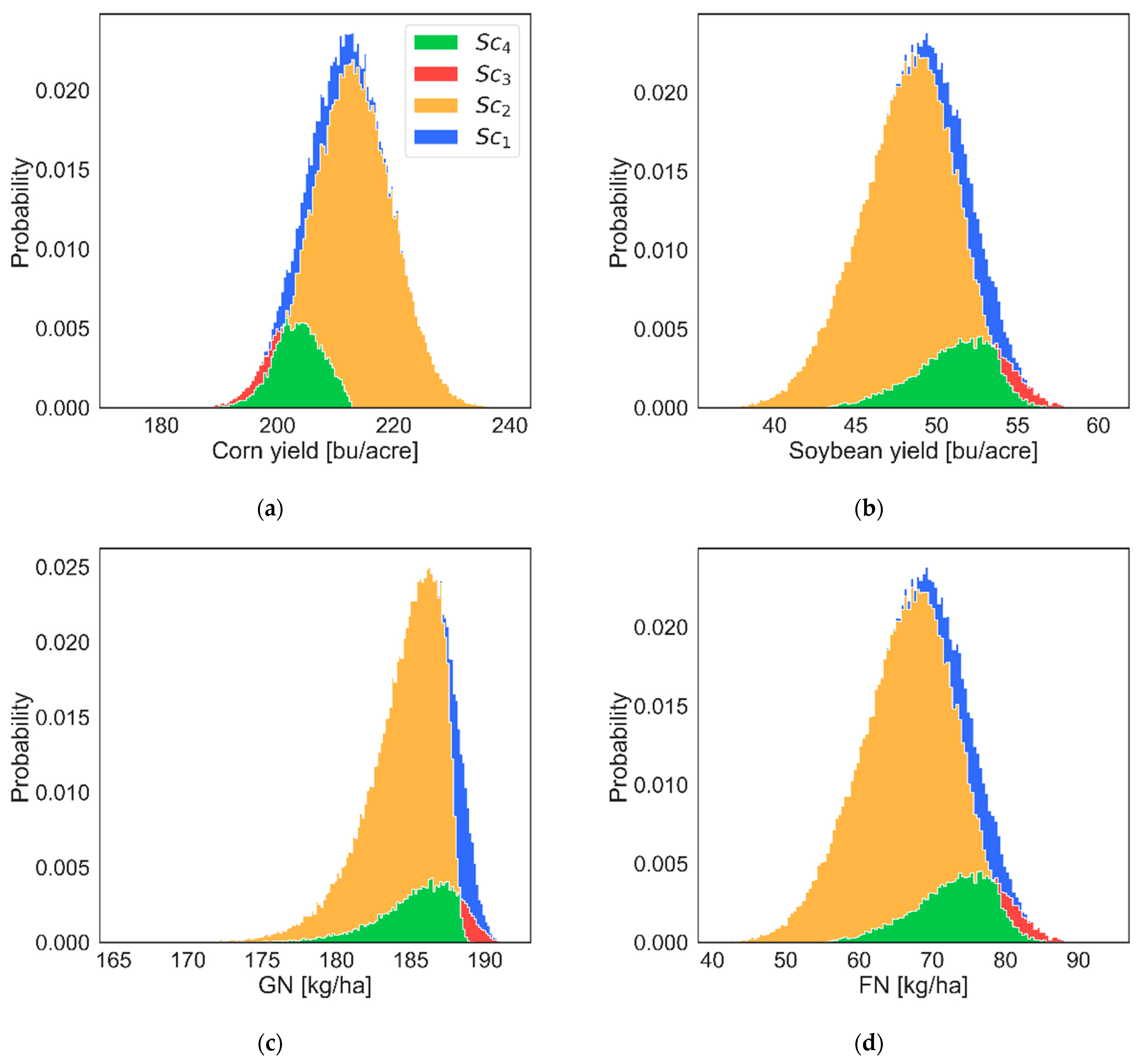
Figure 5 shows the decomposed distribution of corn and soybean yield along with the variation in FN and GN values. The effect of different scenarios due to combinations of weather parameters can be clearly seen in crop yield distribution. It is interesting to note that in dry condition (Sc3) corn yield drops compared to the yield in regular condition, whereas higher soybean yield is observed in dry condition compared to the regular condition. The computation of GN is influenced by both corn and soybean yield values (Figure 5c). The computation of FN is only influenced by soybean yield values (Section 2.2); thus, the FN distribution is observed to be similar to soybean yield distribution.
Figure 6 shows the decomposed distribution of nitrogen surplus (Ns), the final output of the IFEW simulation model. The soil nitrogen surplus is usually affected by CN, MN, GN, and FN magnitudes. However, in this study, only GN and FN influence the variation in nitrogen surplus. This is mainly because the parameters affecting CN and MN are kept constant. The variation in nitrogen surplus shown in this work is purely due to uncertainty in weather parameters. From Figure 6, it is observed that most of the variation in nitrogen surplus lies in regular condition (Sc2), varying approximately between 0 and 20 kg/ha. The scenarios with high July temperatures (Sc3 and Sc4) are observed to produce mid to high nitrogen surplus values. Similarly, scenario Sc1, with very low July precipitation and regular July temperature, tends to produce higher nitrogen surplus than in regular conditions. The dry condition with high July temperature and low July precipitation produces the highest soil nitrogen surplus, varying between 20 and 30 kg/ha. The accumulated nitrogen in the soil is highly water-soluble and could get exported at a high rate to the Mississippi River through melting snow or rainfall before the next growing season. Figure 6 provides the expected magnitude of nitrogen load from state of Iowa to the Mississippi River in different weather scenarios.
The SD in this work uses the Monte Carlo sampling approach which could be used to provide approximate probability of a scenario occurring in any given year considering the assumptions made earlier are true. Based on the data available in the current study, probabilities of scenarios Sc1, Sc2, Sc3, and Sc4 occurring are 0.1, 0.74, 0.02, and 0.12, respectively. The probability of dry condition (Sc3) occurring is lowest whereas regular condition (Sc2) has the highest probability of occurring (Figure 6).
The SD approach implemented in the current study provides valuable results to gauge the impact of weather parameters on soil nitrogen surplus along with crop yields and nitrogen transfer in agriculture systems. However, the particular distributions used for the weather parameters are not data based, and the two input weather parameters are assumed to be independent of each during the Monte Carlo sampling process. Temperature and precipitation are correlated. Thus, there is a possibility that some combination of scenarios may not entirely occur. For example, high precipitation and high temperature may not occur at the same time because with high precipitation, the average temperature drops. Further, the probability distributions of the weather parameters are challenging to estimate as they typically do not have continuous distributions. Thus, it is advisable to use weather generators which have been trained on historical datasets to predict weather parameters rather than using continuous probability distributions. In future studies, weather generators will be included in the IFEW simulation model to predict weather data for more realistic predictions of soil nitrogen surplus.
4. Conclusions
In this work, the simulation decomposition (SD) approach is implemented with the Iowa food-energy-water (IFEW) system simulation model to better understand the impact of weather behavior on nitrogen export from Iowa. In particular, the previously developed nitrogen export model, which computes the soil nitrogen surplus, is extended with a crop weather model to include the dependence of weather in the IFEW system. The updated IFEW simulation model with SD is used to provide decomposed soil nitrogen surplus distribution in different weather scenarios.
It is observed that July temperature and precipitation directly impact corn and soybean yields. Interestingly, it is observed that in the dry condition, corn yield reduces, whereas soybean yield increases compared to the yield values in regular conditions. The variation in crop yields affects nitrogen transfer in the agriculture system through fixation nitrogen (FN) and grain nitrogen (GN), affecting the soil nitrogen surplus. The SD approach provides the distribution of nitrogen surplus in various scenarios. It is observed that the regular condition covers most variation in the full distribution. Scenarios with high July temperature and low precipitation tend to produce mid to high range of nitrogen surplus values. The dry condition scenario produces the highest nitrogen surplus. Overall, the SD approach provides a deeper understanding of the cause-and-effect relationship between weather parameters and soil nitrogen surplus.
Furthermore, the current study identified that continuous distribution on weather parameters could generate unrealistic scenarios. Thus, in future studies, highly validated weather generators will be used for estimating weather parameters, providing a more realistic distribution of soil nitrogen surplus based on weather. Additionally, the IFEW simulation model will be extended to report nitrogen loads for Iowa’s nine crop reporting districts, providing spatially resolved information from the state of Iowa.
Author Contributions
Conceptualization, L.L. and A.K.; methodology, V.R.; software, V.R.; validation, V.R. and Y.-C.L.; writing—original draft preparation, V.R. and Y.-C.L.; writing—review and editing, V.R., Y.-C.L., L.L. and A.K.; visualization, V.R. and Y.-C.L.; supervision, L.L. and A.K. All authors have read and agreed to the published version of the manuscript.
Funding
The United States National Science Foundation under grant No. 1739551.
Institutional Review Board Statement
Not applicable.
Informed Consent Statement
Not applicable.
Data Availability Statement
Not applicable.
Acknowledgments
This material is based upon work supported by the United States National Science Foundation under grant No. 1739551.
Conflicts of Interest
The authors declare no conflict of interest.
References
- Diaz, R.J.; Rosenberg, R. Spreading Dead Zones and Consequences for Marine Ecosystems. Science 2008, 321, 926–929. [Google Scholar] [CrossRef] [PubMed]
- EPA. Northern Gulf of Mexico Hypoxic Zone. Available online: https://www.epa.gov/ms-htf/northern-gulf-mexico-hypoxic-zone (accessed on 2 December 2021).
- Burkart, M.R.; James, D.E. Agricultural-Nitrogen Contributions to Hypoxia in the Gulf of Mexico. J. Environ. Qual. 1999, 28, 850–859. [Google Scholar] [CrossRef]
- Jones, C.S.; Schilling, K.E. Iowa Statewide Stream Nitrate Loading: 2017–2018 Update. J. Iowa Acad. Sci. 2019, 126, 6–12. [Google Scholar] [CrossRef]
- NDEE. Ethanol Facilities’ Capacity by State. Available online: https://neo.ne.gov/programs/stats/inf/121.htm (accessed on 5 December 2021).
- Urbanchuk, J.M. Contribution of the Renewable Fuels Industry to the Economy of Iowa. Agricultural and Biofuels Consulting. Available online: https://iowarfa.org/wp-content/uploads/2020/03/2019-Iowa-Economic-Impact-Final-2.pdf (accessed on 4 December 2021).
- Bakhsh, A.; Kanwar, R.; Karlen, D. Effects of liquid swine manure applications on NO3–N leaching losses to subsurface drainage water from loamy soils in Iowa. Agric. Ecosyst. Environ. 2005, 109, 118–128. [Google Scholar] [CrossRef] [Green Version]
- Siderius, C.; Kolusu, S.R.; Todd, M.C.; Bhave, A.; Dougill, A.J.; Reason, C.J.; Mkwambisi, D.D.; Kashaigili, J.J.; Pardoe, J.; Harou, J.J.; et al. Climate variability affects water-energy-food infrastructure performance in East Africa. One Earth 2021, 4, 397–410. [Google Scholar] [CrossRef]
- Berardy, A.; Chester, M.V. Climate change vulnerability in the food, energy, and water nexus: Concerns for agricultural production in Arizona and its urban export supply. Environ. Res. Lett. 2017, 12, 035004. [Google Scholar] [CrossRef]
- Raul, V.; Leifsson, L.; Kaleita, A. System Modeling and Sensitivity Analysis of the Iowa Food-Water-Energy Nexus. J. Environ. Inform. Lett. 2020, 4, 73–79. Available online: http://www.jeiletters.org/index.php?journal=mys&page=article&op=view&path%5B%5D=202000044 (accessed on 1 August 2021). [CrossRef]
- Westcott, P.C.; Jewison, M. Weather Effects on Expected Corn and Soybean Yields; Feed Outlook No. (FDS-13G-01); USDA Economic Research Service: Washington, DC, USA, 2013. Available online: https://www.ers.usda.gov/publications/pub-details/?pubid=36652 (accessed on 23 November 2021).
- Kozlova, M.; Collan, M.; Luukka, P. Simulation decomposition: New approach for better simulation analysis of multi-variable investment projects. Fuzzy Econ. Rev. 2016, 21, 3–18. [Google Scholar] [CrossRef]
- Kozlova, M.; Yeomans, J.S. Multi-Variable Simulation Decomposition in Environmental Planning: An Application to Carbon Capture and Storage. J. Environ. Inform. Lett. 2019, 1, 20–26. [Google Scholar] [CrossRef] [Green Version]
- Lambe, A.B.; Martins, J.R.R.A. Extensions to the design structure matrix for the description of multidisciplinary design, analysis, and optimization processes. Struct. Multidiscip. Optim. 2012, 46, 273–284. [Google Scholar] [CrossRef]
- USDA. Crop Production 2019 Summary. Crop Production 2019 Summary 01/10/2020 (usda.gov) 2020. Available online: https://www.nass.usda.gov/Publications/Todays_Reports/reports/cropan20.pdf (accessed on 4 December 2021).
- Blesh, J.; Drinkwater, L.E. The impact of nitrogen source and crop rotation on nitrogen mass balances in the Mississippi River Basin. Ecol. Appl. 2013, 23, 1017–1035. [Google Scholar] [CrossRef] [PubMed]
- Barry, D.A.J.; Goorahoo, D.; Goss, M.J. Estimation of Nitrate Concentrations in Groundwater Using a Whole Farm Nitrogen Budget. J. Environ. Qual. 1993, 22, 767–775. [Google Scholar] [CrossRef]
- USDA. National Agricultural Statistics Service Quick Stats. Available online: https://quickstats.nass.usda.gov/ (accessed on 24 November 2021).
- Gronberg, J.M.; Arnold, T.L. County-Level Estimates of Nitrogen and Phosphorus from Animal Manure for the Conterminous United States, 2007 and 2012 (No. 2017-1021); US Geological Survey: Reston, VA, USA, 2017. [CrossRef] [Green Version]
- Jones, C.S.; Drake, C.W.; Hruby, C.E.; Schilling, K.E.; Wolter, C.F. Livestock manure driving stream nitrate. Ambio 2019, 48, 1143–1153. [Google Scholar] [CrossRef] [PubMed]
- Kroese, D.P.; Brereton, T.; Taimre, T.; Botev, Z.I. Why the Monte Carlo method is so important today. WIREs Comput. Stat. 2014, 6, 386–392. [Google Scholar] [CrossRef]
- Kozlova, M.; Yeomans, J.S. Monte Carlo Enhancement via Simulation Decomposition: A “Must-Have” Inclusion for Many Disciplines. INFORMS Trans. Educ. 2020. [Google Scholar] [CrossRef]
- Sawyer, J.E. Nitrogen Use in Iowa Corn Production; Crop 3073; Iowa State University Extention and Outreach: Ames, IA, USA. Available online: https://store.extension.iastate.edu/Product/Nitrogen-Use-in-Iowa-Corn-Production (accessed on 20 November 2021).
- USDA. Fertilizer Use and Price. Available online: https://www.ers.usda.gov/data-products/fertilizer-use-and-price/ (accessed on 29 November 2021).
- McKay, M.D.; Beckman, R.J.; Conover, W. A comparison of three methods for selecting values of input variables in the analysis of output from a computer code. Technometrics 2000, 42, 55–61. [Google Scholar] [CrossRef]
Figure 1.
A model of the interdependencies of the Iowa food-energy-water (IFEW) system.

Figure 2.
An extended design structure matrix diagram of the proposed Iowa nitrogen export model.

Figure 3.
Probability distribution of simulation output for example problem: (a) output full distribution, and (b) decomposed distribution based on scenarios.
Figure 3.
Probability distribution of simulation output for example problem: (a) output full distribution, and (b) decomposed distribution based on scenarios.

Figure 4.
Decomposed distribution of input parameters from simulation decomposition: (a) July temperature (w1), and (b) July precipitation (w2).
Figure 4.
Decomposed distribution of input parameters from simulation decomposition: (a) July temperature (w1), and (b) July precipitation (w2).

Figure 5.
Decomposed distribution of intermittent IFEW model parameters from simulation decomposition: (a) corn yield (x1), (b) soybean yield (x2), (c) GN, and (d) FN.
Figure 5.
Decomposed distribution of intermittent IFEW model parameters from simulation decomposition: (a) corn yield (x1), (b) soybean yield (x2), (c) GN, and (d) FN.

Figure 6.
Distribution of IFEW simulation model output: nitrogen surplus (Ns).


Table 1.
Nitrogen content in manure and life cycle for livestock groups used in manure N calculation [19].
Table 1.
Nitrogen content in manure and life cycle for livestock groups used in manure N calculation [19].
| Livestock Group | Nitrogen in Manure (AMN) (kg per Animal per Day) | Life Cycle (LF) (Days per Year) |
|---|---|---|
| Hog/pigs | 0.027 | 365 |
| Beef cattle | 0.15 | 365 |
| Milk cows | 0.204 | 365 |
| Heifer/steers (0.5 × other cattle) | 0.1455 | 365 |
| Slaughter cattle (0.5 × other cattle) | 0.104 | 170 |
Table 2.
Input parameter details.
| Parameter | Distribution/Range | State | Boundary |
|---|---|---|---|
| U [0, 10] | Low | [0–5) | |
| High | (5–10] | ||
| U [0, 10] | Low | [0–5) | |
| High | (5–10] |
Table 3.
Generating scenarios from parameter states.
| Scenario | Combination of States |
|---|---|
| Sc1 | : Low |
| Sc2 | : High |
| Sc3 | : Low |
| Sc4 | : Low |
Table 4.
Input parameter details for performing simulation decomposition with IFEW simulation model.
Table 4.
Input parameter details for performing simulation decomposition with IFEW simulation model.
| Parameter | Distribution/Range | State | Boundary |
|---|---|---|---|
| July temperature (w1) | N [2, 74] | Regular | ≤76 °F |
| High | >76 °F | ||
| July precipitation (w2) | LogN [0.4, 0, 4] | Regular | ≥2.5 in |
| Low | <2.5 in |
Table 5.
Scenarios for simulation decomposition approach with IFEW model.
| Scenario | Combination of States | Description |
|---|---|---|
| Sc1 | w1: Regular, w2: Low | Regular-T Low-PPT |
| Sc2 | w1: Regular, w2: Regular | Regular condition |
| Sc3 | w1: High, w2: Low | Dry condition |
| Sc4 | w1: High, w2: Regular | High-T Regular-PPT |
Publisher’s Note: MDPI stays neutral with regard to jurisdictional claims in published maps and institutional affiliations. |
© 2022 by the authors. Licensee MDPI, Basel, Switzerland. This article is an open access article distributed under the terms and conditions of the Creative Commons Attribution (CC BY) license (https://creativecommons.org/licenses/by/4.0/).
Share and Cite
MDPI and ACS Style
Raul, V.; Liu, Y.-C.; Leifsson, L.; Kaleita, A. Effects of Weather on Iowa Nitrogen Export Estimated by Simulation-Based Decomposition. Sustainability 2022, 14, 1060. https://0-doi-org.brum.beds.ac.uk/10.3390/su14031060
AMA Style
Raul V, Liu Y-C, Leifsson L, Kaleita A. Effects of Weather on Iowa Nitrogen Export Estimated by Simulation-Based Decomposition. Sustainability. 2022; 14(3):1060. https://0-doi-org.brum.beds.ac.uk/10.3390/su14031060
Chicago/Turabian StyleRaul, Vishal, Yen-Chen Liu, Leifur Leifsson, and Amy Kaleita. 2022. "Effects of Weather on Iowa Nitrogen Export Estimated by Simulation-Based Decomposition" Sustainability 14, no. 3: 1060. https://0-doi-org.brum.beds.ac.uk/10.3390/su14031060
Note that from the first issue of 2016, this journal uses article numbers instead of page numbers. See further details here.