Assessment of PV Module Temperature Models for Building-Integrated Photovoltaics (BIPV)

Abstract

This paper assesses two steady-state photovoltaic (PV) module temperature models when applied to building integrated photovoltaic (BIPV) rainscreens and curtain walls. The models are the Ross and the Faiman models, both extensively used for PV modules mounted on open-rack support structures in PV plants. The experimental setups arrange the BIPV modules vertically and with different backside boundary conditions to cover the mounting configurations under study. Data monitoring over more than a year was the experimental basis to assess each model by comparing simulated and measured temperatures with the help of four different metrics: mean absolute error, root mean square error, mean bias error, and coefficient of determination. The performance ratio of each system without the temperature effect was calculated by comparing the experimental energy output with the energy output determined with the measured temperatures. This parameter allowed the estimation of the PV energy with the predicted temperatures to assess the suitability of each temperature model for energy-prediction purposes. The assessment showed that the Ross model is the most suitable for predicting the annual PV energy in rainscreen and curtain-wall applications. Highlighted is the importance of fitting the model coefficients with a representative set of in situ monitored data. The data set should preferably include the inner (backside) temperature, i.e., the air chamber temperature in ventilated façades or the indoor temperature in curtain walls and windows.

1. Introduction

The integration of photovoltaic energy in buildings (BIPV) has proven to efficiently and aesthetically combine the local generation of renewable electricity with the fulfillment of several construction functions of the building envelope [1,2]. Both in existing buildings and new ones, the possibilities of BIPV solutions are diverse and can significantly contribute to the energy saving of the building [3,4,5,6,7,8]. In the urban context, façades offer a huge potential for BIPV, often higher than roofs [9,10,11]. Ventilated façades (rainscreens) and curtain walls are the most widespread building-envelope systems in commercial buildings and, to a lesser extent, residential buildings. These types of façades are especially suitable to become BIPV façades [12], as many international examples have shown during recent years [1,11,13]. Currently, the market offers a variety of products and solutions to develop successful BIPV rainscreens and curtain walls. Furthermore, recent work on technological BIPV development has reviewed the current materials and BIPV design possibilities [14].

As BIPV grows, it is even more necessary to improve the available tools for the optimal electrical design and simulation of BIPV systems. This means correctly modeling the performance of such BIPV systems, which includes PV module temperature modeling. Over the years, different modeling developments have addressed the PV module operating temperature of free-standing PV modules, as was summarized in [15]. However, in building-integrated systems, the modules are not open-rack-mounted and usually are neither optimally tilted for PV generation nor ventilated as in PV plants. As a consequence, the operating temperatures of PV modules in buildings are in general higher than in PV plants. Since the determination of the module temperature is important for correctly simulating and predicting the performance of PV systems, testing procedures, modeling, and standards have historically addressed module temperature. However, most effort has focused on PV plants and not on PV in buildings. This work aimed to assess to what extent those models are suitable for PV modules integrated in rainscreens and curtain walls or windows.

The article is organized as follows: after a preliminary introduction about BIPV in façades, Section 1 addresses the need to progress in the determination of the BIPV module temperature; Section 2 reviews previous work and background about PV module temperature modeling and states the objectives of the work; Section 3 describes the experimental setups for the rainscreen and the curtain wall, the data monitoring, and the data-filtering process, and the method to assess the models’ accuracy in the prediction of the PV energy; and Section 4 includes the results for the rainscreen and the curtain-wall systems, including the analysis of the impact of the ventilation regime and the considered ambient temperatures, as well as the assessment of the PV energy-prediction accuracy of the models. Next, Section 5 includes the main conclusions of the work. Finally, the nomenclature is included.

2. Background and Objective

Although the detailed study of the photovoltaic (PV) module temperature should include heat-transfer phenomena analysis [16,17], which would lead to transient temperature models, the alternative, analytical steady-state temperature models have been extensively used to determine the PV module temperature in PV plants. These straightforward models only need simple meteorological variables as an input, and led to acceptable degree of accuracy in the prediction of electrical PV performance in PV plants [18]. Some of the proposed models were found to determine the module temperature with an accuracy comparable to the cell-to-cell temperature differences typically encountered within a module [15,19]. This means that these models could be accurate enough to determine an average module temperature to be used in the electrical-performance simulation of PV modules and systems, also because the temperature has a second-order influence on the PV output energy; typically, the output power decreases less than 0.5% by each temperature degree increase (according to [20], between 0.3% and 0.5%).

While in PV plants this approach could be sufficient, in building-integrated photovoltaic (BIPV) and building-added photovoltaic (BAPV) systems the thermal-performance-accuracy requirement might be higher, e.g., for building energy simulation. However, it is worth assessing the suitability of these temperature models for electrical-performance-simulation purposes. Thus far in the literature, a few works have addressed the analysis of some of these simple models to certain particular mounting conditions of BIPV or BAPV [21,22,23], mainly in roof applications [24]. For example, Assoa et al. [25] focused on the thermal characterization of semi-integrated PV roof systems, finding that not only the developed heat-transfer-based models, both 2-D dynamic and steady-state models, but also a simple linear model, achieved a good prediction of the PV module temperature.

The most extended temperature model in the PV sector has been the Ross model [26] (see Equation (1)). It assumes a linear proportionality of the difference between PV module and ambient temperatures (T_m−T_a) and the plane of array (module) irradiance, G_POA. For each set of boundary conditions, the constant k is characteristic of the module design and materials, as experimentally shown in some publications [27]. The IEC PV standards adopted the Ross model to define the nominal operating cell temperature (NOCT) [28] as the characteristic temperature reached by the cells in the module at the open-circuit state under the following conditions: 800 W m⁻² irradiance, 20 °C ambient temperature, 1 m/s wind speed, module tilt angle of 37 degrees, and open-air ventilation (Equation (2)). Thus, the Ross coefficient k would correspond to k = (NOCT-20)/800 (Equation (2)).

$$T_{\mathrm{m}}=T_{ \mathrm{a}}+k\cdot G_{POA}$$

(1)

$$T_{\mathrm{m}}=T_{\mathrm{a}}+\frac{NOCT-20}{800}\cdot G_{POA}$$

(2)

To extend the suitability of the NOCT model to other mounting conditions, SANDIA National Laboratories defined the Installed Nominal Operating Cell Temperature (INOCT), a more realistic approach for the determination of the nominal operating temperature under different mounting conditions [21]. Similarly, ‘effective NOCT’ (NOCT_eff) was the term used by the authors in [23] to name the NOCT fitted at the specific operating conditions of a BIPV ventilated façade.

Table 1. Ross coefficient (k) values found in the literature [22,29] and tentative corresponding effective nominal operating temperatures (NOCT_eff).

PV Array Mounting Type, Module Type	k (°C m2/W)	NOCTeff (°C)
Free-standing	0.021	36.8
Flat roof	0.026	40.8
Sloped roof, well-cooled	0.020	36.0
Sloped roof, not-so-well-cooled	0.034	47.2
Sloped roof, highly integrated and poorly ventilated	0.056	64.8
Façade-integrated, semitransparent PV	0.046	56.8
Façade-integrated with narrow gap, opaque PV	0.054	63.2

includes some examples for the Ross coefficient, given by [22] and based on [29] data, corresponding to some different module and mounting types. A column with the corresponding effective NOCT values has been added, which aims at relating both parameters.

The addition of the wind-speed effect in steady-state temperature models was intended to improve their accuracy. The Faiman model [30] included two parameters to fit, one describing the wind speed dependence and the other the irradiance dependence (see Equation (3)). Skoplaki [6] slightly changed this model to include a third parameter dependent on the mounting solution. Some years later, IEC standards substituted NOCT by the Faiman model adapted to some specific boundary conditions stated in the IEC 61853-2 standard [31] (Equation (3)).

$$T_{\mathrm{m}}=T_{\mathrm{a}}+\frac{G_{POA}}{u_0+u_1{W}_s}$$

(3)

In Equation (3), T_a is the ambient dry bulb temperature, G_POA is the plane of array irradiance, W_s is the wind speed, and $u_0$ and $u_1$ are two empirical parameters to be fitted for each module. The boundary conditions are similar to those of NOCT, but with the module operating at the maximum power point instead of at the open-circuit state. In this case, the module temperature obtained with Equation (3) at T_a = 20 °C, G_POA = 800 W/m², and W_s = 1 m/s is the nominal module operating temperature (NMOT) [13]. Analogously to the case of NOCT_eff, the suffix ‘eff’ applied to NMOT (NMOT_eff) means ‘effective’ and indicates that NMOT was calculated by fitting the model parameters at some other boundary conditions; in this case, at vertical position (tilt angle 90°) and with different rear ventilation regimes.

Different works have assessed NOCT and NMOT models, generally considering open-rack-mounted modules [18,32], but some of them addressing related BIPV configurations also. For instance, Davis et al. [33] concluded that the NOCT model underpredicted the module temperatures and found temperature differences of up to 20 degrees between insulated and non-insulated vertically mounted modules. Measured and predicted insulated module temperatures could differ significantly during a day, depending on the type of day (i.e., clear or cloudy). Other studies have tried to establish specific boundary conditions to standardize the procedure to determine NMOT for BIPV [34].

From the review, it can be concluded that these two models are straightforward to use (more the NOCT than the NMOT), but they have some accuracy limitations when applied to short periods (e.g., days) due to the coefficients’ dependence on the environmental conditions. This work hypothesizes that, despite the above-mentioned limitations, these models can be sufficiently accurate for predicting the annual BIPV performance of BIPV façades if the coefficients are fitted at the real BIPV system or with the help of suitable setups under the local environmental conditions.

The objective of this work was to assess the above described steady-state models for their use in BIPV façades where PV modules become curtain-wall or rainscreen elements. Another goal was to study which is the most convenient experimental temperature to consider as the ambient temperature (T_a) in these simple models when applied to BIPV solutions, since the front (outdoor) and back air temperatures surrounding the modules are different.

3. Methodology

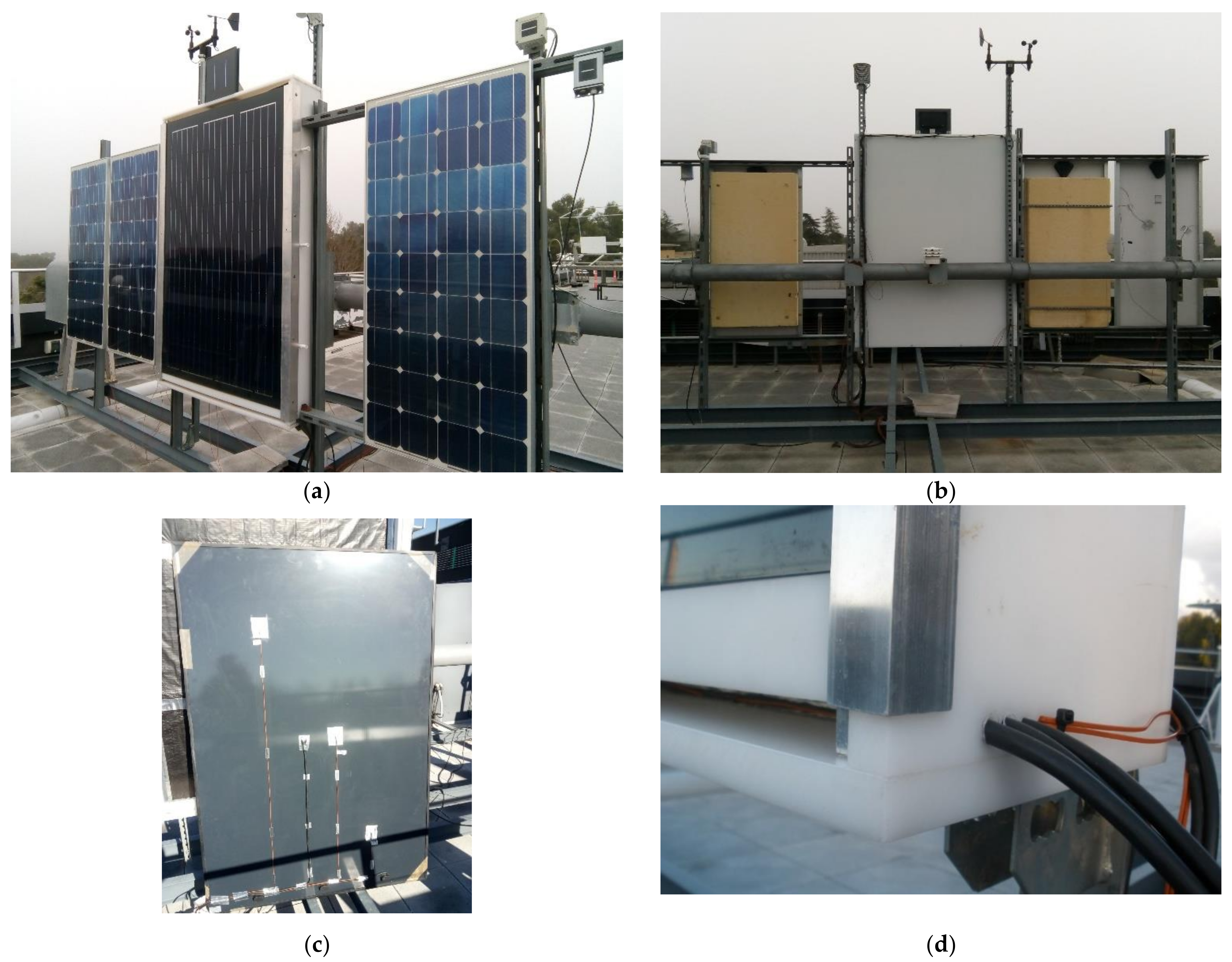
3.1. Rainscreen Experimental Setup

The experimental setup for the rainscreen case study is shown in Figure 1. It consists of three similar single-crystalline silicon (sc-Si) standard PV modules and one multicrystalline silicon (mc-Si) BIPV module mounted in a mock-up that simulates the boundary conditions of a ventilated façade. This mock-up was designed in the framework of a round-robin international research activity conducted in IEA-PVPS Task 15 [35], and served for the PV annual energy comparison among nine different sites spread over the world [36]. It consists of a mounting enclosure with a 10 cm air chamber on the back and two air apertures, up and down, for natural convective ventilation of the PV module. The PV module (module A in the present work) is an Ertex Solar VSG-L with 54 square mc-Si cells (156 mm side each), a glass/glass laminate structure using polyvinyl butyral (PVB) as the encapsulant, and a colored enamel coating at the back.

The three sc-Si modules Atersa A-120 P5 have a conventional glass/Tedlar structure (modules B). One of them has free ventilation on its back (module B_{total V}), but in the other two cases, a 7 cm-thick extruded polystyrene sheet is either in contact with the module back sheet (module B_{not V}) or creating a 5 cm ventilated air chamber (module B_{partial V}), emulating a ventilated façade solution. See Figure 1a,b.

Module temperatures were measured with several thermocouples placed on their back sheets in positions coincident with the middle of the cells. The ambient temperature, the plane of array irradiance, and the wind speed were the other monitored parameters. Concerning module A, the temperature of the air chamber was also monitored at two different heights. While the three type-B modules were open-circuited, module A was grid-connected through a microinverter, which kept this module at maximum power point (MPP) condition.

Solar irradiance was measured using an Atersa crystalline silicon reference cell, with an uncertainty of ±3%. Ambient temperature and PV module temperature were measured using T-type thermocouples, with an uncertainty of ±1 °C for a coverage probability of 95% assuming a normal distribution. Wind speed was measured with an anemometer Young 05103, with an accuracy of ±0.3 m/s.

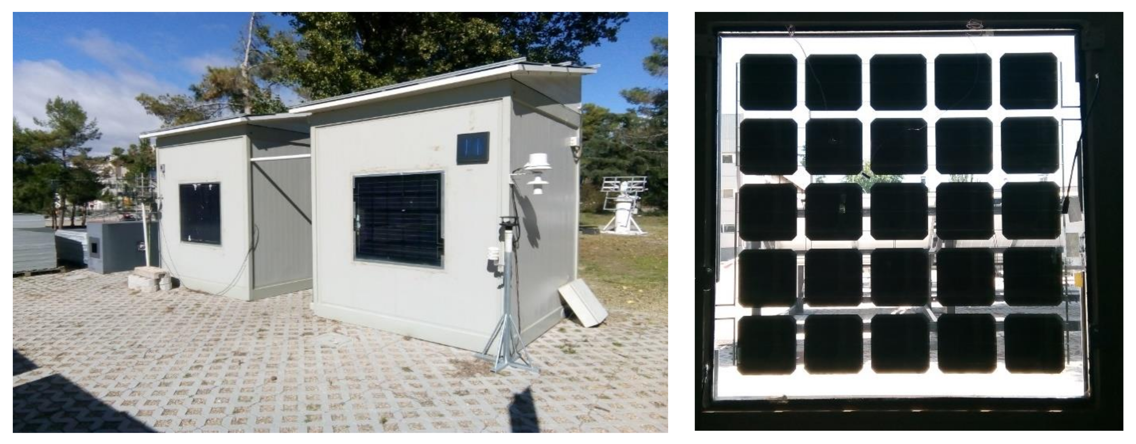
3.2. Curtain-Wall Experimental Setup

For the case of a BIPV curtain wall, the setup consisted of two semitransparent PV (STPV) modules mounted as windows in the south façades of two identical testing cabins. This CIEMAT testing facility was designed for testing and monitoring BIPV modules under real operating conditions in the framework of the OMEGA-CM R&D Program [http://projects.ciemat.es/web/omega-cm/] (see Figure 2). It allows comparison of the behavior of two products and has been useful for the development and validation of heat-transfer temperature and thermal transmittance models [37]. Although these are not curtain walls, the boundary conditions of these two PV windows are very similar to those of a curtain wall; moreover, the two modules are designed as BIPV curtain-wall elements.

In the present study, the monitored parameters were: in-plane solar irradiance measured with two calibrated PV cells, ambient temperature (indoor and outdoor), wind speed, module temperature, and output voltage and current at the maximum power point set by a grid-connected microinverter. The monitoring time step was one minute, and the accuracy of the measurements was similar to that of the rainscreen setup.

The two BIPV modules were custom-manufactured by Yingli Solar. They are semitransparent, 1 m × 1 m in size, and made of 25 bifacial n-type sc-Si cells. One of these modules has a laminated glass structure (PVLG): glass/EVA/PV cells/EVA/glass, while the other is a double-glazing unit (PVDG): glass/PVB/PV cells/PVB/glass/air chamber/inner glass pane.

3.3. Data Monitoring and Filtering

For the rainscreen setup, the monitoring time step was 1 minute, and the measurement period was 18 months. For the curtain wall setup, the monitoring time step was 0.5 minute, and the measurement period was 9 months. One third of the data were used for the models fitting, and the rest of them for the prediction assessment. The data analysis from these studies for the NOCT and NMOT models followed the filtering procedures included in the international standards [28,31].

For the NOCT case, data taken under the following conditions were rejected:

• Irradiance below 400 W/m²;
• In a 10 min interval after the irradiance varied by more than 10% from the maximum value to the minimum value recorded during that 10 min period;
• Wind speed outside the range 1 m/s ± 0.75 m/s;
• Ambient temperature outside the range 20 °C ± 15 °C.

For the NMOT case, data taken under the following conditions were rejected:

• Irradiance below 400 W/m²;
• In a 10 min interval after the irradiance varied by more than 10% from the maximum value to the minimum value during the preceding 10 min period;
• In a 10 min interval from a deviation of the instantaneous wind speed to below 0.25 m/s or gusts larger than + 200% from a 5 min running average;
• When the 5 min running average was less than 1 m/s or greater than 8 m/s.

Filtering data in the case of window PV modules was similar to the case of rainscreen elements. However, an additional filtering criterion was imposed prior to the mentioned filtering conditions to avoid partial shading effects. The two calibrated cells for monitoring the incident solar irradiance data were used to ensure that all used data correspond to no-shading conditions in both PV windows, by rejecting data for which relative difference between the two solar irradiance signals was higher than 10%.

After data filtering, the parameters of each model were fitted by linear regression. In the NMOT case, the parameters were obtained by considering G_POA/(–_m − T_a) as a variable dependent on the wind speed.

3.4. Method for the Assessment of the Energy-Prediction Accuracy of the Models

Model fitting by linear regression returned predicted temperatures and fitting errors (i.e., mean absolute error, root mean square error, mean bias error, and coefficient of determination). Besides, we compared the experimental PV energy with the predicted PV energy when using the predicted module temperatures also taking into account the performance ratio of the PV system. In general, the PV energy (E_PV) generated by a PV system can be expressed as:

$$E_{\mathrm{PV}}=\left[\frac{P_{\mathrm{p}}}{G_{\mathrm{ref}}} \cdot H_{\mathrm{POA}}\right]\cdot PR,$$

(4)

where P_p is the peak power of the PV array (in this case, the PV module), which is the maximum power at the standard test conditions (STC), G_ref is the STC irradiance (1 kW/m²), H_POA is the plane of array irradiation, and PR is the performance ratio of the system, which shows the effect of the PV system losses on the generated PV energy. Thus, the expression in brackets represents the theoretical generated energy just considering the irradiation the BIPV module receives. The performance ratio of a PV system can be divided into two coefficients, one related to the temperature loss (PR_T) and the other (PR_o) related to the rest of the losses (spectral, angular, wiring, inverter, …):

$$PR=P{R}_{\mathrm{o}}\cdot P{R}_{\mathrm{T}}$$

(5)

To determine PR_o, we compared the experimental PV energy (E_PV^exp) with the theoretical PV energy calculated by using the experimental module temperature (E_PV^Tm-exp):

$${\mathrm{PR}}_{\mathrm{o}}=\frac{{\mathrm{E}}_{\mathrm{PV}}{}^{\exp }}{{\mathrm{E}}_{\mathrm{PV}}{}^{\mathrm{Tm}-\exp }}=\frac{({\sum }_{\mathrm{k}}{\mathrm{P}}_{\mathrm{out,k}}\cdot {\mathsf{\tau }}_{\mathrm{k}})}{({\sum }_{\mathrm{k}}{\mathrm{P}}_{\mathrm{p}}\cdot ({\mathrm{G}}_{\mathrm{POA}}/{\mathrm{G}}_{\mathrm{ref}})\cdot \left(1+\mathsf{\gamma } \cdot \left({\mathrm{T}}_{\mathrm{m}-\mathrm{e}\mathrm{x}\mathrm{p},\mathrm{k}}– 25\right)\right)\cdot {\mathsf{\tau }}_{\mathrm{k}})},$$

(6)

where P_out,k is the PV system average output power in the time interval k, γ is the relative maximum-power temperature coefficient (°C⁻¹), T_m-exp,k is the module temperature (°C) measured in the time interval k, and τ_k is the time interval duration.

Once PR_o is determined, it is possible to compare the PV energy calculated with the modeled module temperature (E_PV^Tm-model) (Equation (7)) with the experimental PV energy output.

$$E_{\mathrm{PV}}{}^{T\mathrm{m}-\mathrm{model}}=\left({\displaystyle \sum _{\mathrm{k}}}{P}_{\mathrm{p}}\cdot (G_{POA}/G_{\mathrm{ref}})\cdot \left(1+\gamma \cdot \left(T_{m-model,k}– 25\right)\right)\cdot {\tau }_{\mathrm{k}}\right)\cdot P{R}_{\mathrm{o}}$$

(7)

This allows the assessment of the temperature models’ accuracy in predicting the PV energy output. Hence, prediction errors are calculated in reference to the measured experimental values:

$$\epsilon \left(\%\right) =100\cdot (E_{\mathrm{PV}}{}^{\exp }-E_{\mathrm{PV}}{}^{T\mathrm{m}-\mathrm{model}})/E_{\mathrm{PV}}{}^{\exp }$$

(8)

4. Results and Discussion

4.1. Results for BIPV Ventilated Façade Systems

4.1.1. Influence of the Ventilation Regime

We fitted half-year monitoring data of the three similar type-B modules, all in open-circuit condition but with different ventilation regimes (denoted as modules B_{total V}, B_{not V}, and B_{partial V}), to the Ross and Faiman models. Then, the obtained coefficients were used to predict module temperatures during another year of measurements, and these modeled temperatures were compared with the experimental ones. The results are shown in

Table 2. Results of the Ross model for the three ventilation regimes applied to module B.

Module	R2	MAE (°C)	RMSE (°C)	MBE (°C)	NOCTeff (°C)
Btotal V	0.90	2.8	3.7	−2.0	44.1
Bnot V	0.90	4.1	5.6	−0.5	61.3
Bpartial V	0.85	4.1	5.5	−2.8	55.1

and

Table 3. Results of the Faiman model for the three ventilation regimes applied to module B.

Module	R2	MAE (°C)	RMSE (°C)	MBE (°C)	u0 (W/m2 °C)	u1 (Ws/m3 °C)	NMOTeff (°C)
Btotal V	0.84	3.6	4.7	1.7	69.4	2.93	31.1
Bnot V	0.74	6.7	8.7	4.6	28.7	0.97	47.0
Bpartial V	0.75	5.0	7.0	3.2	39.9	1.58	39.3

, respectively.

For the Ross model, as Table 2 shows, the coefficient of determination of the linear regression (R²) is high in all cases, especially in the fully ventilated and non-ventilated cases. Considering that the experimental average temperature difference between any two different cells in the module is ±2 °C, we conclude that the mean average error (MAE) is low in the ventilated case (2.8 °C) and acceptable in the other two cases (4.1 °C). However, prediction with the model is biased towards lower values, especially in the totally ventilated and semi-ventilated cases, where the mean bias error (MBE) is −2 °C and −2.7 °C, respectively. The obtained NOCT_eff values vary between 44.1 °C and 61.6 °C from the totally ventilated case to the non-ventilated case, that is, a temperature difference of 17.5 °C. All the rest of eventual situations would fall between these two extreme values, as is the case of B_{partial V} (NOCT_eff = 55.1 °C). Similar NOCT values have been reported in Malaga, Spain, under similar climate conditions (i.e., Mediterranean, Csa-type climate): 62.7 °C for stand-alone (i.e., ventilated) conditions and 45.6 °C for rear-side-isolated (i.e., non-ventilated) conditions, resulting in a temperature difference of 17.1 °C [38].

When applying the Faiman model to module B, with the three different ventilation regimes and in the open-circuit state, we obtain the results shown in Table 3. For the totally and partially ventilated cases, R² and MAE show acceptable results (being worse in the partially ventilated case), although RMSE indicates a slightly lower prediction accuracy if compared to the Ross model. Results for the non-ventilated case are not so good. In all cases, the model overestimates the module temperature (i.e., MBE is a positive value). In addition, the low influence of the wind speed (i.e., a low u₁ value) can be observed in the non-ventilated case.

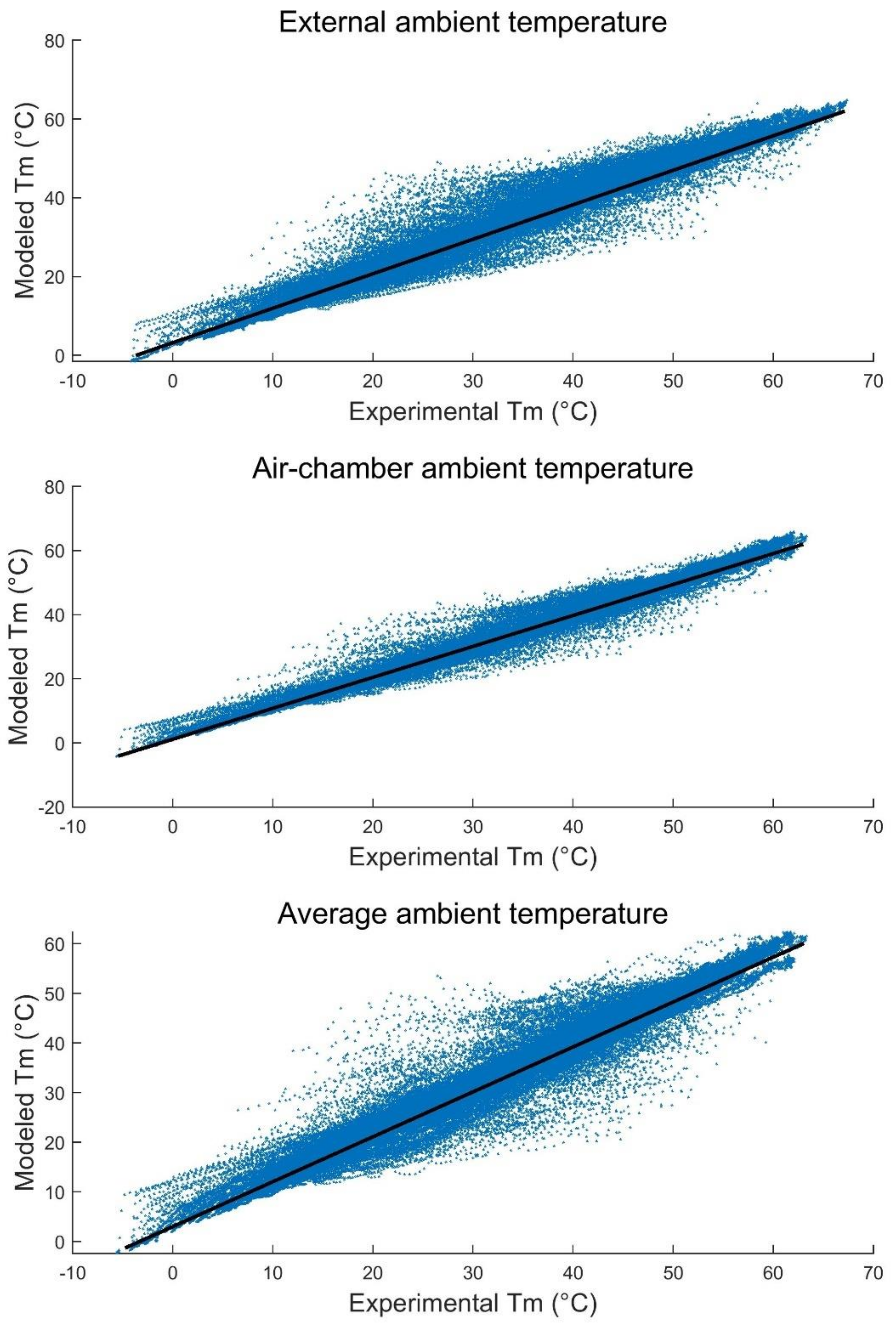
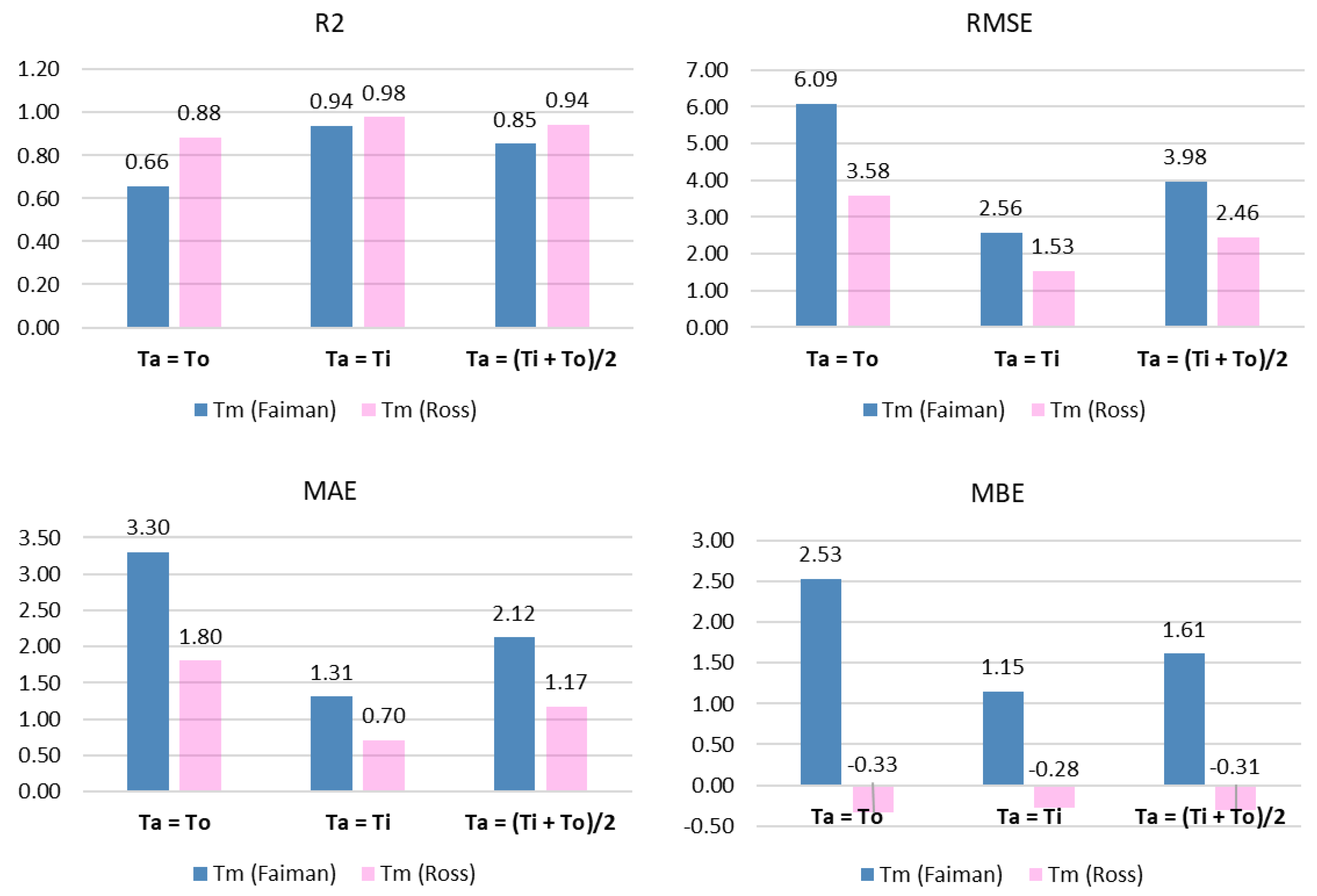
4.1.2. Influence of the Considered Surrounding Ambient Temperature

Module A was monitored together with the three type-B modules, although the module A data set also included its electrical output parameters (voltage and current at the MPP) and the two surrounding average temperatures (air chamber and outdoor). The three ambient-temperature inputs considered when applying the Ross and Faiman models to module A were the back-chamber air temperature (T_i), the outdoor ambient temperature (T_o), or the average between both of them ((T_i + T_o)/2). Figure 3 shows the scatter plot corresponding to the Ross model, and Figure 4 contains the fit results for both models and the three ambient temperatures.

As observed, the best results were obtained when considering the back air temperature, achieving high R² and low RMSE and MAE values with both models. Results were still good when considering the average ambient temperature with the Ross model and acceptable with the Faiman model. In all cases, the Ross model shows better fitting results. Again, the Faiman model overestimated the module temperature, and the Ross model slightly underestimated it.

The fitted NOCT_eff value decreases when considering the back inner temperature: 51.1 °C for the outdoor temperature, 36.5 °C for the air chamber temperature, and 49.8 °C for the average of both temperatures.

4.1.3. Impact of Results on the PV Energy-Prediction Accuracy

To evaluate the impact of the different temperature models on the electrical output of the BIPV ventilated façade element, we followed the methodology described in the Introduction section (Equations (4) to (8)). The obtained PR_o value for the module A rainscreen system is 0.89.

Table 4. Errors in the prediction of the annual PV energy of the ventilated façade mockup with the Faiman model and the Ross model.

Considered Ambient Temperature	εFaiman (%)	εRoss (%)
Outdoor ambient temperature (To)	3.06	−0.45
Air chamber temperature (Ti)	1.32	−0.39
Average temperature (Ti, To)	1.94	−0.39

shows the calculated errors in the annual PV energy estimation for each considered ambient temperature and temperature model.

It is worth noting that the relative error in the energy yield prediction is low in all cases, although significantly lower (absolute values under 0.5%) when using the Ross temperature model. This model slightly underestimates the energy output of the PV system, while the Faiman model overestimates it.

According to these results, the Ross model is suitable with any of the ambient temperatures (back or front) to achieve good energy-prediction results. However, it is recommendable to measure the air-chamber temperature to improve the prediction accuracy.

4.2. Results for BIPV Curtain Walls

The results of applying the two models to the BIPV windows are shown in Figure 5 and Figure 6, where the considered ambient temperature was the outdoor temperature. As it can be seen, the results are quite similar for the two models. As expected, models work better for the case of the simple glass laminate than for the double-glazing one since the latter displays higher thermal inertia.

Table 5. Ross fitting results for the PV laminated glass (PVLG) and the PV double glazing (PVDG) if considering the outdoor temperature (T_o), the indoor temperature (T_i), or the average of both of them. The modules’ electrical state is MPP.

Ambient Temperature	R2		MAE (°C)		RMSE (°C)		MBE (°C)		NOCTeff (°C)
	PVLG	PVDG	PVLG	PVDG	PVLG	PVDG	PVLG	PVDG	PVLG	PVDG
indoor (Ti)	0.98	0.95	0.8	1.3	1.3	1.9	0.2	−1.0	43.2	43.9
outdoor (To)	0.92	0.78	2.4	4.2	2.6	4.4	2.1	4.1	47.4	39.5
average (Ti, To)	0.96	0.94	1.5	1.9	1.6	2.1	1.1	1.6	39.3	41.7

includes the results for the Ross model, considering the outdoor, indoor, or average temperatures.

From Table 5, it can be observed that monitoring the indoor ambient temperature instead of the outdoor ambient temperature increases the accuracy of the model. However, results for the PVLG are good in all cases. Regarding the impact on the PV output, the prediction error is lower than 1% in all cases.

5. Conclusions

The proposed methodology allows the assessment of PV module temperature models applied to BIPV modules integrated into rainscreens and curtain walls or windows. This work studied the suitability of Ross and Faiman models, and, as a general conclusion, both showed good fitting results. However, the Ross model performed better in all the considered cases, so the inclusion of the wind-speed effect (Faiman model) did not increase the fitting accuracy. One possible reason is that wind only affects one face of the modules in BIPV rainscreens, curtain walls and windows.

Monitoring the indoor ambient temperature for the case of BIPV curtain walls or windows and the air chamber temperature for the rainscreen case improved the fitting results of the models.

The methodology includes a way to study the impact of the PV module temperature accuracy on the BIPV system output prediction. In our case studies, the obtained errors in predicting the annual PV energy were lower than 1% with the Ross model and between 1% and 3% with the Faiman model. Thus, the Ross model was the most suitable for predicting BIPV rainscreen and curtain-wall system performance.

Regarding the procedure to determine the model coefficients, we recommend using in situ monitored data, preferably including the inner ambient temperature: the air chamber temperature in ventilated façades or the indoor temperature in curtain walls or windows. The fitted parameters, especially the NOCT_eff for each case, can help to improve the accuracy of the electrical simulation tools when applied to those types of BIPV systems.

As a final conclusion, the results of this study have shown that the Ross and Faiman temperature models can be suitable for calculating the PV yield of BIPV systems such as rainscreens, curtain walls, and windows. The accuracy in the determination of the module temperature was sufficient for correctly simulating and predicting the performance of the BIPV systems over the periods considered.

References

1. Reijenga, T.; Ritzen, M.; Scognamiglio, A.; Kappel, K.; Frontini, F.; Moor, D.; Schneider, A.; Illich, P.; Delisle, V.; Kapsis, K.; et al. Successful Building Integration of Photovoltaics—A Collection of International Projects, International Energy Agency. 2020. Available online: https://iea-pvps.org/wp-content/uploads/2021/03/IEA-PVPS-Task-15-An-international-collection-of-BIPV-projects-compr.pdf (accessed on 15 December 2021).
2. Corti, P.; Bonomo, P.; Frontini, F.; Macé, P.; Bosch, E. Building Integrated Photovoltaics: A Practical Handbook for Solar Buildings’ Stakeholders. Status Report. 2020. Available online: https://solarchitecture.ch/wp-content/uploads/2020/11/201022_BIPV_web_V01.pdf (accessed on 28 December 2021).
3. Olivieri, L.; Caamaño-Martín, E.; Moralejo-Vázquez, F.J.; Martín-Chivelet, N.; Olivieri, F.; Neila-Gonzalez, F.J. Energy saving potential of semi-transparent photovoltaic elements for building integration. Energy 2014, 76, 572–583. [Google Scholar] [CrossRef] [Green Version]
4. Miyazaki, T.; Akisawa, A.; Kashiwagi, T. Energy savings of office buildings by the use of semi-transparent solar cells for windows, Renew. Energy 2005, 30, 281–304. [Google Scholar] [CrossRef]
5. Cornaro, C.; Basciano, G.; Puggioni, V.A.; Pierro, M. Energy saving assessment of semi-transparent photovoltaic modules integrated into NZEB. Buildings 2017, 7, 9. [Google Scholar] [CrossRef] [Green Version]
6. Peng, J.; Curcija, D.C.; Lu, L.; Selkowitz, S.E.; Yang, H.; Zhang, W. Numerical investigation of the energy saving potential of a semi-transparent photovoltaic double-skin facade in a cool-summer Mediterranean climate. Appl. Energy 2016, 165, 345–356. [Google Scholar] [CrossRef]
7. Lu, L.; Law, K.M. Overall energy performance of semi-transparent single-glazed photovoltaic (PV) window for a typical office in Hong Kong, Renew. Energy 2013, 49, 250–254. [Google Scholar] [CrossRef]
8. Ng, P.K.; Mithraratne, N.; Kua, H.W. Energy analysis of semi-transparent BIPV in Singapore buildings. Energy Build. 2013, 66, 274–281. [Google Scholar] [CrossRef]
9. Redweik, P.; Catita, C.; Brito, M. Solar energy potential on roofs and facades in an urban landscape. Sol. Energy 2013, 97, 332–341. [Google Scholar] [CrossRef]
10. Desthieux, G.; Carneiro, C.; Camponovo, R.; Ineichen, P.; Morello, E.; Boulmier, A.; Abdennadher, N.; Dervey, S.; Ellert, C. Solar energy potential assessment on rooftops and facades in large built environments based on lidar data, image processing, and cloud computing. Methodological background, application, and validation in geneva (solar cadaster). Front. Built Environ. 2018, 4, 14. [Google Scholar] [CrossRef]
11. Aranda-Mena, G.; Fong, T.P. Building Integrated Photovoltaic for Architectural Façades in Singapore. J. Sustain. Res. 2020, 2, 1–19. [Google Scholar] [CrossRef]
12. Attoye, D.E.; Aoul, K.A.T.; Hassan, A. A review on building integrated photovoltaic façade customization potentials. Sustainability 2017, 9, 2287. [Google Scholar] [CrossRef] [Green Version]
13. Martín-Chivelet, N.; Gutiérrez, J.C.; Alonso-Abella, M.; Chenlo, F.; Cuenca, J. Building retrofit with photovoltaics: Construction and performance of a BIPV ventilated façade. Energies 2018, 11, 1719. [Google Scholar] [CrossRef] [Green Version]
14. Kuhn, T.E.; Erban, C.; Heinrich, M.; Eisenlohr, J.; Ensslen, F.; Neuhaus, D.H. Review of technological design options for building integrated photovoltaics (BIPV). Energy Build. 2020, 231, 110381. [Google Scholar] [CrossRef]
15. Skoplaki, E.; Palyvos, J.A. Operating temperature of photovoltaic modules: A survey of pertinent correlations. Renew. Energy 2009, 34, 23–29. [Google Scholar] [CrossRef]
16. Wong, P.W.; Shimoda, Y.; Nonaka, M.; Inoue, M.; Wah, W.P.; Shimoda, Y.; Nonaka, M.; Inoue, M. Field study and modeling of semi-transparent PV in power, thermal and optical aspects. J. Asian Arch. Build. Eng. 2005, 4, 549–556. [Google Scholar] [CrossRef] [Green Version]
17. Fung, T.Y.; Yang, H. Study on thermal performance of semi-transparent building-integrated photovoltaic glazings. Energy Build. 2008, 40, 341–350. [Google Scholar] [CrossRef]
18. Bae, J.H.; Kim, D.Y.; Shin, J.W.; Lee, S.E.; Kim, K.C. Analysis on the Features of NOCT and NMOT Tests with Photovoltaic Module. IEEE Access 2020, 8, 151546–151554. [Google Scholar] [CrossRef]
19. Faiman, D. Assessing the outdoor operating temperature of photovoltaic modules. Prog. Photovolt. Res. Appl. 2008, 16, 307–315. [Google Scholar] [CrossRef]
20. Stein, J.S.; Schroedter-Homscheidt, M.; De Brabandere, K.; Suri, M.; Remund, J.; Sengupta, M.; Lorenz, E.; Driesse, A.; Winter, S.; Hammer, A.; et al. PV Performance Modeling Methods and Practices. Results from the 4th PV Performance Modeling Collaborative Workshop. Report IEA-PVPS T13-06:2017. 2017. Available online: https://iea-pvps.org/wp-content/uploads/2020/01/T13_Report_PV_Performance_Modeling_Methods_and_Practices_FINAL_March_2017.pdf (accessed on 13 December 2021).
21. Fuentes, M. A Simplified Thermal Model for Flat-Plate Photovoltaic Arrays. Report Number: SAND-85-0330 ON: DE87009386. 1987. Available online: https://www.osti.gov/biblio/6802914 (accessed on 13 December 2021).
22. Skoplaki, E.; Boudouvis, A.G.; Palyvos, J.A. A simple correlation for the operating temperature of photovoltaic modules of arbitrary mounting. Sol. Energy Mater. Sol. Cells 2008, 92, 1393–1402. [Google Scholar] [CrossRef]
23. Payno, D.; Chivelet, N.M.; Cuenca, J. Temperatura de operación nominal efectiva de módulos fotovoltaicos en integración arquitectónica. In Proceedings of the XVI Congreso Ibérico y XII Congreso Iberoamericano de Energía Solar, Madrid, Spain, 20–22 June 2018. [Google Scholar]
24. D’Orazio, M.; di Perna, C.; di Giuseppe, E. Experimental operating cell temperature assessment of BIPV with different installation configurations on roofs under Mediterranean climate. Renew. Energy 2014, 68, 378–396. [Google Scholar] [CrossRef]
25. Assoa, Y.B.; Mongibello, L.; Carr, A.; Kubicek, B.; Machado, M.; Merten, J.; Misara, S.; Roca, F.; Sprenger, W.; Wagner, M.; et al. Thermal analysis of a BIPV system by various modelling approaches. Sol. Energy 2017, 155, 1289–1299. [Google Scholar] [CrossRef] [Green Version]
26. Ross, R.G. Interface design considerations for terrestrial solar cell modules. In Proceedings of the IEEE Photovoltaic Specialists Conference, Baton Rouge, LA, USA, 15 November 1976; pp. 801–806. [Google Scholar]
27. Maturi, L.; Belluardo, G.; Moser, D.; del Buono, M. BiPV system performance and efficiency drops: Overview on PV module temperature conditions of different module types. Energy Procedia 2014, 48, 1311–1319. [Google Scholar] [CrossRef] [Green Version]
28. International Electrotechnical Commission. Terrestrial photovoltaic (PV) modules—Design qualification and type approval (IEC Standard No. 61215:2005); International Electrotechnical Commission: Geneva, Switzerland, 2005. [Google Scholar]
29. Nordmann, T.; Clavadetscher, L. Understanding temperature effects on PV system performance. In Proceedings of the Third World Conference on Photovoltaic Energy Conversion, Osaka, Japan, 11–18 May 2003; pp. 2243–2246. [Google Scholar]
30. International Electrotechnical Commission. Terrestrial photovoltaic (PV) modules—Design qualification and type approval—Part 2: Test procedures (IEC Standard No. IEC 61215:2016); International Electrotechnical Commission: Geneva, Switzerland, 2016. [Google Scholar]
31. International Electrotechnical Commission. IEC 61853-2:2016 Photovoltaic (PV) Module Performance Testing and Energy—Part 2: Spectral Responsivity, Incidence Angle and Module Operating Temperature Measurements. 2016. Available online: https://webstore.iec.ch/publication/25811#additionalinfo (accessed on 28 December 2021).
32. Muller, M.; Marion, B.; Rodriguez, J. Evaluating the IEC 61215 Ed.3 NMOT procedure against the existing NOCT procedure with PV modules in a side-by-side configuration. In Proceedings of the Conference Record of the 2012 38th IEEE Photovoltaic Specialists Conference, Austin, TX, USA, 3–8 June 2012; pp. 697–702. [Google Scholar] [CrossRef]
33. Davis, M.W.; Fanney, A.H.; Dougherty, B.P. Prediction of Building Integrated Photovoltaic Cell Temperatures*. J. Sol. Energy Eng. 2001, 123, 200–210. [Google Scholar] [CrossRef]
34. Wei, C.G.; Pan, R.N.; Wang, D. Research of Nominal Operating Temperature Testing Method of BIPV Module. Key Eng. Mater. 2017, 726, 18–22. [Google Scholar] [CrossRef]
35. Gaisberger, L.; Rechberger, P.; Eder, G.; Berger, K.A.; Gusztáv, Ú.; Illich, P.; Moor, D.; Boddaert, S.; Bonomo, P.; Valckenborg, R.; et al. BIPV round robin action of IEA-PVPS Task 15. In Proceedings of the 36th European Photovoltaic Solar Energy Conference and Exhibition, Marseille, France, 9–13 September 2019; pp. 1815–1820. Available online: https://www.photovoltaic-conference.com/59-eu-pvsec-2019.html (accessed on 11 December 2021).
36. Gaisberger, L.; Valckenborg, R.; Berger, K.A.; Újvári, G.; Eder, G.C.; Illich, P.; López, C.S.S.B.P.; del Buono, M.; Chivelet, N.M.; Martinez, A.S.; et al. IEC 61853-matrix analysis of PVPS Task 15 BIPV round-robin for more than one year at seven test sites over the world. In Proceedings of the 37th European Photovoltaic Solar Energy Conference and Exhibition, Lisbon, Portugal, (online), 7–11 September 2020; pp. 1719–1725. [Google Scholar]
37. Misara, S.; Henze, N.; Sidelev, A. Thermal Behaviours of BIPV-Modules (U-Value and g-Value). In Proceedings of the 26th European Photovoltaic Solar Energy Conference and Exhibition (26th EU PVSEC), Hamburg, Germany, 5–9 September 2011; pp. 4107–4115. [Google Scholar]
38. Sanchez-Friera, P.; Fernández, M.; Piliougine, M.; Sidrach-de-Cardona, M. Influence of Design Parameters on the Nominal Operation Cell Temperature of PV modules. In Proceedings of the 25th European Photovoltaic Solar Energy Conference and Exhibition/5th World Conference on Photovoltaic Energy Conversion, Valencia, Spain, 6–10 September 2010; pp. 4253–4256. [Google Scholar]
Figure 1. Different views of the rainscreen experimental setup. (a) Front view of the four vertically mounted PV modules. From left to right: Btotal V, Bnot V, A, and Bpartial V. (b) Back view of the four vertically mounted PV modules. From right to left: Btotal V, Bnot V, A, and Bpartial V. (c) Backside of the mc-Si BIPV module (module A) before mounting, showing the thermocouples positions. (d) Detail of the mock-up with the bottom ventilation air gap.
Sustainability 14 01500 g001
Figure 2. (Left) South façades of the two testing cabins with the semitransparent BIPV modules, and (right) a view of the PVDG module from the inside.
Sustainability 14 01500 g002
Figure 3. For module A, modeled temperature with the Ross model versus experimental temperature. Each graph corresponds to the indicated ambient-temperature-input selection. Results are analyzed in Figure 4.
Sustainability 14 01500 g003
Figure 4. Coefficient of determination (R2), root mean square error (RMSE), mean absolute error (MAE), and mean bias error (MBE) for the Faiman and Ross models when considering three different ambient temperatures: the outdoor temperature (To), the air chamber temperature (Ti), and the average of both.
Sustainability 14 01500 g004
Figure 5. Scatter plots of modeled versus experimental temperature for the photovoltaic laminated glass (PVLG).
Sustainability 14 01500 g005
Figure 6. Scatter plots of modeled versus experimental temperature for the photovoltaic double glazing (PVDG).
Sustainability 14 01500 g006