Stability Analysis of Continuous Stochastic Linear Model

Abstract

Many scholars have conducted research on the traffic oscillations and reproduced the growth pattern by establishing stochastic models and simulations. However, the growth pattern of oscillations caused by uncertainty have not been thoroughly studied. Recently, a frequency domain stability analysis method was proposed to analyze the discrete stochastic model. This paper extends this analysis to a continuous situation based on frequency domain tools (e.g., Laplace transform) by introducing a continuous bandlimited white noise. The analytical expression for the evolution of speed standard deviation has been derived. Our study of a homogeneous case reveals an interesting phenomenon: when ${\left|G\left(\omega \right)\right|}_{\infty }<1$, the speed variance will converge to a constant value, which only depends on the self-disturbance of vehicles. The simulation results verified that the continuous models and corresponding discrete model tend to be consistent when the discrete time step tends to the infinitesimal. Overall, this paper makes up for the deficiency of previous studies on continuous oscillations in car-following theory and can potentially be used to develop new control strategies to help dampen traffic oscillations.

1. Introduction

In the last century, the research on traffic flow mainly focused on the classical models. The early exploration in this field can be traced back to 1953. Pipes [1] used a differential dynamics equation to describe car-following behavior and assumed that there is a positive correlation between the speed difference and the following vehicle acceleration, in other words, when the speed of the preceding vehicle is greater/lower than that of the following vehicle, the following vehicle will accelerate/decelerate. Newell [2] took the distance between the preceding and following vehicle into account and proposed that the speed of the following vehicle is positively correlated with the distance. Furthermore, Bando et al. [3] proposed that there exists an ‘optimal velocity’ determined by that distance. He also proposed that the acceleration of the following vehicle should be related to the ‘optimal velocity’ and the current velocity. Based on this optimal velocity model, Hilbing and Tilch [4] developed a generalized force model by considering the negative velocity difference to avoid unrealistic deceleration. Jiang et al. [5] considered both negative and positive velocity difference and developed a full velocity model. A nonlinear analysis method was proposed by Xue et al. [6] with a full velocity model by which a reasonable kinematics wave speed can be obtained. Zhao et al. [7] accounted for acceleration and proposed a full velocity and acceleration difference model (FVADM). Nagatani [8,9,10] and Sawada [11] extended the car-following model with a next-nearest neighbor interaction.

Although these classic models have clear and elegant stability properties, the growth pattern of oscillation is inconsistent with the field experiment, in which the speed standard deviation of each vehicle developed concavely. Jiang et al. established 2D models by changing the deterministic parameters to stochastic and successfully simulated the concave pattern in 2014 [12]. Lang et al. [13] improved the inertia model and proposed that the amplitudes of car accelerations become larger along the car platoon; Xu et al. [14] presented an analysis of a Newell-type stochastic car-following model based on the stochastic desired acceleration processes. After which, a number of stochastic car-following models were developed [15,16,17,18].

From another point of view, bottlenecks and lane-changing have been believed to be the main causes of traffic oscillations [19,20,21,22] until Sugiyama’s experiment [23], which shows traffic oscillations occurred in the absence of lane changing/bottlenecks. However, researchers are still in debate about traffic oscillations being a result of the string instabilities in the mathematical models [24,25,26] or heterogeneous driving behavior [27,28,29]. This paper put forward another view that the traffic oscillations are caused not by the model or heterogeneous behavior, but by the disturbance of the drivers/vehicles itself.

In 2020, Wang et al. [30] proposed the frequency-domain stability analysis method for linear stochastic car-following models, extending the traditional frequency domain analysis tool of the deterministic model to stochastic models. This method is able to quantify speed variations of a stream of vehicles following one another according to certain stochastic linear car-following behaviors. However, this method is only applicable in a time-discrete condition, which is inconsistent with the fact that physical time should be continuous. Motivated by the fact, this paper extends the abovementioned method to the first-order model under time-continuous circumstance to verify whether this method is still feasible. We also discussed the feasibility for extending this model to second-order models. Our study of the homogeneous case reveals that when traffic is stable, the speed variance converges to a constant value, which only depends on the self-disturbance of drivers/vehicles. The simulation results verified that the continuous models and corresponding discrete model tend to be consistent when discrete time step tends to the infinitesimal. The continuous models and corresponding discrete model tend to be consistent in our simulations. Overall, this paper fills the gap in the research of continuous noise in traffic-flow theory and could potentially be used to develop new control strategies to help in dampening traffic oscillations.

The organization of this paper is as follows. In Section 2, the continuous stochastic linear First-order model is described. In Section 3, the stability analysis method is performed and reveals the relationship between the discrete and continuous model. In Section 4, numerical examples are provided to illustrate the application of the proposed method to continuous stochastic linear first-order models. Section 5 concludes this paper and discusses future research directions.

2. Model

Assuming that a vehicle platoon with an index of n = 1,2,3…, N moves on a single lane without any overtaking as shown in Figure 1, we use $\mathcal{N}$ to denote the index set {1,2,3…, N} for convenience.

We introduce the definition of string stability as follows: the string of a vehicle is stable if, for any set of bounded initial disturbances to all the vehicles, the position fluctuations of all the vehicles remain bounded [31]. For the convenience of the readers, the key notation is summarized in

Table 1. Notation List.

Notation	Definition	Notation	Definition
N	total vehicle number	$r_1\left(\xi \right)$	the autocorrelation function of $v_1\left(t\right)$
$\mathcal{N}$	vehicle index set	$S_1\left(\omega \right)$	power density
$v_n^0\left(t\right)$	the speed of the $n\mathrm{th}$ vehicle at time t	$V_n\left(s\right)$	Laplace transformation of $v_n\left(t\right)$
$p_n^0\left(t\right)$	the position of the $n\mathrm{th}$ vehicle at time $t$	$G_n\left(s\right)$	transfer function between the n−1 and nth vehicle
$v_n\left(t\right)$	the speed of the $n\mathrm{th}$ vehicle at time $t$ after linearization	${\overline{\Delta }}_n$	speed variance of the $n$th vehicle under DFM
$p_n\left(t\right)$	the position of the $n\mathrm{th}$ vehicle at time $t$ after linearization	${\Delta }_n$	speed variance of the $n$th vehicle under SFM
${\alpha }_n$	Constant coefficient	${\widehat{\Delta }}_n$	simulate speed variance under DFM
$\tau$	reaction time	${\tilde{\Delta }}_n$	simulate speed variance under SFM
${\epsilon }_n\left(t\right)$	continuous bandlimited white noise	${\acute{\Delta }}_n$	noise term (continuous condition)
${\sigma }_n^2$	variance of white noise ${\epsilon }_n\left(t\right)$	${\stackrel{`}{\Delta }}_n$	noise term (Discrete condition)

.

We use $v_n^0\left(t\right), p_n^0\left(t\right)$ to denote the speed and position of the $n$th vehicle at time $t$. Assuming that at the initial time $t=0$, all vehicles are in a stationary condition, which implies the same starting speed $\overline{v}$ and corresponding spacing ${\overline{p}}_n$, i.e.:

$$v_n^0\left(0\right)=\overline{v},p_{n-1}^0\left(0\right)-p_n^0\left(0\right)={\overline{p}}_n,\forall n\in \mathcal{N}$$

(1)

Since this article focuses on the study of oscillation, we convert the variables as follows according to the predecessor’s method [30]:

$$v_n\left(t\right)≔v_n^0\left(t\right)-\overline{v},p_n\left(t\right)≔p_n^0\left(t\right)-p_n^0\left(0\right)-\overline{v}t,\forall n\in \mathcal{N}$$

(2)

Assuming all vehicles follow the stochastic first-order model (SFM):

$$\mathrm{SFM}:v_n\left(t+\tau \right)={\alpha }_n\left(p_{n-1}\left(t\right)-p_n\left(t\right)\right)+{\epsilon }_n\left(t\right), \forall n\in \mathcal{N}\backslash 1$$

(3)

where $\tau$ is the reaction time and the definition of${\epsilon }_n\left(t\right)$ is as follows:${\epsilon }_n\left(t\right)$ is a continuous bandlimited white noise with a variance of ${\sigma }_n^2$ defined on $\left(0~T\right),\left(T\to \infty \right)$ with equal spectral density $E_n$ at different angular frequencies $\left(0~\mathbb{F}\right),\left(\mathbb{F}\to \infty \right)$, which means ${\epsilon }_n\left(t\right)$ satisfies the following equations:

$$\underset{T\to \infty }{lim}\frac{1}{T}{{\displaystyle \int }}_0^T{\left|{\epsilon }_n\left(t\right)\right|}^{2}dt={\sigma }_n^2$$

(4)

$$\left|E_n\left(\omega \right)\right|=\{\begin{array}{c}{E}_n, if 0\le \omega <F \\ 0, otherwise\end{array}$$

(5)

where $E_n\left(\omega \right)$ is the Fourier transform of ${\epsilon }_n\left(t\right)$, i.e.: $E_n\left(\omega \right):=\underset{T\to \infty }{lim}{\int }_0^T{\epsilon }_n\left(t\right)e^{-j\omega t}dt.$ It is worth noting that the reason we do not use a continuous unlimited white noise is that an unlimited white noise has infinite variance, which is not realistic. To analyse the SFM, we define the deterministic first-order model (DFM) as follows:

$$\mathrm{DFM}:v_n\left(t+\tau \right)={\alpha }_n\left(p_{n-1}\left(t\right)-p_n\left(t\right)\right), \forall n\in \mathcal{N}\backslash 1$$

(6)

3. Stability Analysis

3.1. Deterministic Stability Analysis

In this subsection, the task is to obtain the speed variance of the $n$th vehicle under DFM. The Laplace transformation of $v_n\left(t\right)$ can be written as follows:

$$V_n\left(s\right)≔{{\displaystyle \int }}_0^{\infty }{v}_n\left(t\right)e^{-st}dt$$

(7)

Applying the Laplace transformation to both sides of Equation (6), we can obtain the Laplace form of DFM as follows:

$$\left(s{e}^{\tau s}+{\alpha }_n\right)V_n\left(s\right)={\alpha }_n{V}_{n-1}\left(s\right), \forall n\in \mathcal{N}\backslash 1$$

(8)

Thus, the relation between the $\left(i-1\right)$th vehicle velocity disturbance and the $i$th vehicle velocity disturbance is described by:

$$V_n\left(s\right)=G_n\left(s\right)V_{n-1}\left(s\right), \forall n\in \mathcal{N}\backslash 1$$

(9)

where the transfer function $G_n\left(s\right)$ of DFM is:

$$G_n\left(s\right)=\frac{{\alpha }_n}{s{e}^{\tau s}+{\alpha }_n}$$

(10)

According to Parseval’s theorem, we could obtain

$$\underset{T\to \infty }{lim}{{\displaystyle \int }}_0^T{\left|v_n\left(t\right)\right|}^{2}dt=\frac{1}{2\pi }{{\displaystyle \int }}_{-\infty }^{\infty }{\left|V_n\left(j\omega \right)\right|}^{2}d\omega$$

(11)

where $j$ is the imaginary unite and $s=j\omega$. We use $V_n\left(\omega \right)$ to denote $V_n\left(j\omega \right)$ in the following. Dividing both sides of Equation (11) by $T\left(T\to \infty \right)$, we can transform Parseval’s theorem to the following form (which is also the definition of average power $P_n$):

$$\underset{T\to \infty }{lim}{{\displaystyle \int }}_0^T{\left|v_n\left(t\right)\right|}^{2}dt=\frac{1}{2\pi }{{\displaystyle \int }}_{-\infty }^{\infty }{\left|V_n\left(j\omega \right)\right|}^{2}d\omega$$

(12)

$$P_n=\underset{T\to \infty }{lim}\frac{1}{T}{{\displaystyle \int }}_0^T{\left|v_n\left(t\right)\right|}^{2}dt=\frac{1}{2\pi }{{\displaystyle \int }}_{-\infty }^{\infty }\underset{T\to \infty }{lim}\frac{1}{T}{\left|V_n\left(\omega \right)\right|}^{2}d\omega$$

(13)

Noting that in the middle part of Equation (13) is the speed variance of the $n$th vehicle under DFM, and $\underset{T\to \infty }{lim}\frac{1}{T}{\left|V_n\left(\omega \right)\right|}^2$ is the power density of $v_n\left(t\right)$, i.e.:

$${\overline{\Delta }}_n≔\underset{T\to \infty }{lim}\frac{1}{T}{{\displaystyle \int }}_0^T{\left|v_n\left(t\right)\right|}^{2}dt$$

(14)

$$S_n\left(\omega \right)≔\underset{T\to \infty }{lim}\frac{1}{T}{\left|V_n\left(\omega \right)\right|}^2$$

(15)

we can denote Equation (13) as:

$${\overline{\Delta }}_n=\frac{1}{2\pi }{{\displaystyle \int }}_{-\infty }^{\infty }{S}_n\left(\omega \right)d\omega$$

(16)

and also, we can obtain:

$$S_n\left(\omega \right)={\displaystyle \prod }_{m=2}^n{\left|G_m\left(\omega \right)\right|}^2{S}_1\left(\omega \right)$$

(17)

where $S_1\left(\omega \right)$ can be obtained by the Wiener–Khinchin theorem [32]: the autocorrelation function has a spectral decomposition provided by the power spectrum of that process, i.e.:

$$S_1\left(\omega \right)={{\displaystyle \int }}_{-\infty }^{\infty }{r}_1\left(\xi \right)e^{-j\omega \xi }d\xi$$

(18)

where $r_1\left(\xi \right)$ is the autocorrelation function of $v_1\left(t\right)$, i.e.,:

$$r_1\left(\xi \right)≔E\left[v_1\left(t\right)·v_1\left(t+\xi \right)\right]$$

(19)

To achieve $r_1\left(\xi \right)$, we set three leading vehicle cases as follows:

Case 1: $v_1\left(t\right)=A_0\sin \left({\omega }_{0}t\right)$:

$$r_1\left(\xi \right)=E\left[A_0\sin \left({\omega }_{0}t\right)·A_0\sin \left({\omega }_0\left(t+\xi \right)\right)\right]=\frac{A_0^2}{2}\cos \left({\omega }_0\xi \right)$$

(20)

Then, we can easily obtain $S_1\left(\omega \right)$ and ${\overline{\Delta }}_n$ through Equations (15), (16) and (18):

$$S_1\left(\omega \right)=\frac{A_0^2\pi }{2}\left(\delta \left(\omega -{\omega }_0\right)+\delta \left(\omega +{\omega }_0\right)\right)$$

(21)

$${\overline{\Delta }}_{\mathrm{n}}=\frac{A_0^2}{2}{\displaystyle \prod }_{m=2}^n{\left|G_m\left({\omega }_0\right)\right|}^2$$

(22)

Case 2: $v_1\left(t\right)$ is a finite summation of the trigonometric functions:

$$v_1\left(t\right)={\displaystyle \sum }_{k=1}^K{a}_k\sin \left({\omega }_{k}t\right) \left({\omega }_k\ne {\omega }_{l}ifk\ne l\right)$$

(23)

The autocorrelation function can be derived as follows, according to the orthogonality of trigonometric functions:

$$r_1\left(\xi \right)={\displaystyle \sum }_{k=1}^{K}E\left[a_k\sin \left({\omega }_{k}t\right)·a_k\sin \left({\omega }_k\left(t+\xi \right)\right)\right]={\displaystyle \sum }_{k=1}^K\frac{a_k^2}{2}\cos \left({\omega }_k\xi \right)$$

(24)

Then, $S_1\left(\omega \right)$ can be derived using Equation (18), and ${\overline{\Delta }}_{\mathrm{n}}$ can be derived using Equations (16) and (17):

$$S_1\left(\omega \right)={\displaystyle \sum }_{k=1}^K\frac{a_k^2\pi }{2}\left(\delta \left(\omega -{\omega }_k\right)+\delta \left(\omega +{\omega }_k\right)\right)$$

(25)

$${\overline{\Delta }}_n={\displaystyle \sum }_{k=1}^K\frac{a_k^2}{2}{\displaystyle \prod }_{m=2}^n{\left|G_m\left({\omega }_k\right)\right|}^2$$

(26)

From the above equation, we can derive the following proposition:

Proposition 1:

If the leading vehicle moves as$v_1\left[i\right]=\sum _{k=1}^K{f}_k\left[i\right]$, and$f_k\left[i\right]$are orthogonal, then

$${\overline{\Delta }}_{\mathrm{n}}={\displaystyle \sum }_{k=1}^K{\overline{\Delta }}_{nk}$$

(27)

where${\overline{\Delta }}_{nk}$ is the speed variance of the$$th vehicle with the leading vehicle move as$f_k\left[i\right]$ under DFM.

Case 3: $v_1\left(t\right)$ is a bandlimited white noise as defined in Section 2, with a variance of ${\sigma }_1^2$:

By using definition of the Fourier transform of ${\epsilon }_n\left(t\right)$, i.e., $E_n\left(\omega \right)≔\underset{T\to \infty }{lim}{\int }_0^T{\epsilon }_n\left(t\right)e^{-j\omega t}dt$, according to Parseval’s theorem, we can obtain:

$$\underset{T\to \infty }{lim}{{\displaystyle \int }}_0^T{\left|{\epsilon }_n\left(t\right)\right|}^{2}dt=\frac{1}{2\pi }{{\displaystyle \int }}_{-\infty }^{\infty }{\left|E_n\left(\omega \right)\right|}^{2}d\omega$$

(28)

Speed variance can be derived by dividing both sides by $T$:

$${\sigma }_n^2=\underset{T\to \infty }{lim}\frac{1}{T}{{\displaystyle \int }}_0^T{\left|{\epsilon }_n\left(t\right)\right|}^{2}dt=\underset{T\to \infty }{lim}\frac{1}{2\pi T}{{\displaystyle \int }}_{-\infty }^{\infty }{\left|E_n\left(\omega \right)\right|}^{2}d\omega$$

(29)

According to Equation (5), we can derive the following equation:

$$\underset{T\to \infty }{lim}\frac{1}{2\pi T}{{\displaystyle \int }}_{-\infty }^{\infty }{\left|E_n\left(\omega \right)\right|}^{2}d\omega =\underset{T\to \infty }{lim}\underset{\mathbb{F}\to \infty }{lim}\frac{1}{2\pi T}{{\displaystyle \int }}_0^{\mathbb{F}}{\left|E_n\right|}^{2}d\omega$$

(30)

Therefore:

$${\sigma }_n^2=\underset{T\to \infty }{lim}\underset{\mathbb{F}\to \infty }{lim}\frac{1}{2\pi T}{{\displaystyle \int }}_0^{\mathbb{F}}{\left|E_n\right|}^{2}d\omega \Rightarrow {\left|E_1\right|}^2=\underset{T\to \infty }{lim}\underset{\mathbb{F}\to \infty }{lim}\frac{2\pi T{\sigma }_1^2}{\mathbb{F}}$$

(31)

$$S_1\left(\omega \right)=\underset{T\to \infty }{lim}\frac{1}{T}{\left|E_1\left(\omega \right)\right|}^2=\{\begin{array}{c}\underset{\mathbb{F}\to \infty }{lim}\frac{{\sigma }_n^{2}2\pi }{\mathbb{F}}, if 0\le \omega <F \\ 0, otherwise\end{array}$$

(32)

Then, we can easily and ${\overline{\Delta }}_n$ through Equations (15) and (16):

$${\overline{\Delta }}_n=\frac{1}{2\pi }{{\displaystyle \int }}_{-\infty }^{\infty }{\displaystyle \prod }_{m=2}^n{\left|G_m\left(\omega \right)\right|}^2{S}_1\left(\omega \right)d\omega =\underset{\mathbb{F}\to \infty }{lim}\frac{{\sigma }_n^2}{ \mathbb{F}}{{\displaystyle \int }}_0^{ \mathbb{F}}{\displaystyle \prod }_{m=2}^n{\left|G_m\left(\omega \right)\right|}^{2}d\omega$$

(33)

It is obvious that ${\left|G_n\left(\omega \right)\right|}^2\to 0$ as $\omega \to \infty$, thus ${\overline{\Delta }}_n=\underset{\mathbb{F}\to \infty }{lim}\frac{{\sigma }_n^2}{ \mathbb{F}}{{\displaystyle \int }}_0^{ \mathbb{F}}{\displaystyle \prod }_{m=2}^n{\left|G_m\left(\omega \right)\right|}^{2}d\omega =0$ when $n\ge 2$.

3.2. Stochastic Stability Analysis

By applying Fourier transform to the $\mathrm{SFM}$ Equation (3), we can obtain the frequency-domain equation as:

$$V_n\left(\omega \right)=V_{n-1}\left(\omega \right)G_n\left(\omega \right)+H\left(\omega \right)E_n\left(\omega \right)$$

(34)

where $H\left(\omega \right)=\frac{j\omega }{j\omega e^{\tau j\omega }+{\alpha }_n}$, with recursion to Equation (28), we obtain:

$$V_n\left(\omega \right)={\displaystyle \prod }_{m=2}^n{G}_m\left(\omega \right)V_1\left(\omega \right)+{\displaystyle \sum }_{m=2}^n{\displaystyle \prod }_{m^{\prime }=m+1}^n{G}_{m^{\prime }}\left(\omega \right)·H\left(\omega \right)E_n\left(\omega \right)$$

(35)

Therefore, the power density $S_n\left(\omega \right)$ of $v_n\left[i\right]$ can be formulated as:

$$S_n\left(\omega \right)={\displaystyle \prod }_{m=2}^n{\left|G_m\left(\omega \right)\right|}^2{S}_1\left(\omega \right)+\underset{T\to \infty }{lim}\frac{1}{T}{\displaystyle \sum }_{m=2}^n{\displaystyle \prod }_{m^{\prime }=m+1}^n{\left|G_{m^{\prime }}\left(\omega \right)\right|}^2·{\left|E_m\left(\omega \right)H\left(\omega \right)\right|}^2$$

(36)

Because ${\Delta }_n=\frac{1}{2\pi }{\int }_{-\infty }^{\infty }{S}_n\left(\omega \right)d\omega$, the speed variance can be expressed as follows:

$${\Delta }_n={\overline{\Delta }}_n+\underset{\mathbb{F}\to \infty }{lim}\frac{{\sigma }_n^2}{\mathbb{F}}{{\displaystyle \int }}_0^{\mathbb{F}}{\displaystyle \sum }_{m=2}^n{\displaystyle \prod }_{m^{\prime }=m+1}^n{\left|G_{m^{\prime }}\left(\omega \right)\right|}^2·{\left|H\left(\omega \right)\right|}^{2}d\omega$$

(37)

where ${\overline{\Delta }}_n$ can be found in Equations (22), (26) and (33) for all three cases.

3.3. Discussion on Second Order Model

In this section, we apply the above method to second order models to analyze feasibility. To achieve the above purpose, we use the stochastic linear optimal velocity model [3] as an example:

$$a_n\left[i+d_n\right]={\beta }_n\left({\alpha }_n\left(p_{n-1}\left[i\right]-p_n\left[i\right]\right)-v_n\left[i\right]\right)+{\epsilon }_n\left(t\right),\forall n\in \mathcal{N}\backslash 1$$

(38)

Thus, we can conduct the transfer function and the speed variance of the $n$th vehicle under the Homogeneous case as follows:

$$G\left(s\right)=\frac{\alpha \beta }{e^{\tau s}{s}^2+\beta s+\alpha \beta }$$

(39)

$${\Delta }_n={\overline{\Delta }}_n+{\acute{\Delta }}_n$$

(40)

where ${\acute{\Delta }}_n=\underset{\mathbb{F}\to \infty }{lim}\frac{{\sigma }^2}{\mathbb{F}}{\int }_0^{\mathbb{F}}\frac{\left(1-{\left|G\left(\omega \right)\right|}^{2\left(n-1\right)}\right)·{\left|H\left(\omega \right)\right|}^2}{\left(1-{\left|G\left(\omega \right)\right|}^2\right)}d\omega$ and $H\left(\omega \right)=\frac{j\omega }{-e^{\tau s}{\omega }^2+\beta j\omega +\alpha \beta }$, it is obvious that $\left|H\left(\omega \right)\right|\to 0$ and $(1-{\left|G\left(\omega \right)\right|}^2)\to 1$ as $\omega \to \infty$, thus ${\acute{\Delta }}_n=0$ for $n\in \mathcal{N}$, which means that the stochastic term has no effect on the speed variance under the stochastic linear optimal velocity model. The reason for the different effects is that the transfer function has a second order term for the denominator of the second order model, which leads to $\left|H\left(\omega \right)\right|\to 0$ as $\omega \to \infty$, but for the first-order model, $\left|H\left(\omega \right)\right|\to 1$ as $\omega \to \infty$.

3.4. Homogeneous Case Analysis

We assume that all the vehicles have the same transfer function and white noise factor, which means:

$$G_n\left(\omega \right)=G\left(\omega \right),\forall n\in \mathcal{N}\backslash 1$$

(41)

$${\sigma }_n^2={\sigma }^2{E}_n=E,\forall n\in \mathcal{N}\backslash 1$$

(42)

By plugging Equations (41) and (42) to Equations (22), (26), (33) and (37), the speed variance for the homogeneous scene under DFM and SFM could be expressed as follows:

$${\overline{\Delta }}_n=\frac{A_0^2}{2}{\left|G\left({\omega }_0\right)\right|}^{2\left(n-1\right)}\left(\mathrm{Case}1\mathrm{for}\mathrm{DFM}\right)$$

(43)

$${\overline{\Delta }}_n={\displaystyle \sum }_{k=1}^K\frac{a_k^2}{2}{\left|G\left({\mathsf{\omega }}_k\right)\right|}^{2\left(n-1\right)}\left(\mathrm{Case}2\mathrm{for}\mathrm{DFM}\right)$$

(44)

$${\overline{\Delta }}_n=\{\begin{array}{c}0 if n\ge 2\\ {\sigma }_1^2 if n=1\end{array}\left(\mathrm{Case}3\mathrm{for}\mathrm{DFM}\right)$$

(45)

$${\Delta }_n={\overline{\Delta }}_n+\underset{\mathbb{F}\to \infty }{lim}\frac{{\sigma }_n^2}{\mathbb{F}}{{\displaystyle \int }}_0^{\mathbb{F}}{\displaystyle \sum }_{m=2}^n{\left|G\left(\omega \right)\right|}^{2\left(n-m\right)}·{\left|H\left(\omega \right)\right|}^{2}d\omega \left(\mathrm{Cases}1–3\mathrm{for}\mathrm{SFM}\right)$$

(46)

Noticing ${\left|G\left(\omega \right)\right|}^{2\left(n-m\right)}·{\left|H\left(\omega \right)\right|}^2$ is a geometric series, we obtain:

$${\Delta }_n={\overline{\Delta }}_n+\underset{\mathbb{F}\to \infty }{lim}\frac{{\sigma }^2}{\mathbb{F}}{{\displaystyle \int }}_0^{\mathbb{F}}\frac{\left(1-{\left|G\left(\omega \right)\right|}^{2\left(n-1\right)}\right)·{\left|H\left(\omega \right)\right|}^2}{\left(1-{\left|G\left(\omega \right)\right|}^2\right)}d\omega$$

(47)

Proposition 2:

From the above equation, it is obvious that when${\left|G\left(\omega \right)\right|}_{\infty }>1$,${\Delta }_n\to \infty$as$n\to \infty$; when${\left|G\left(\omega \right)\right|}_{\infty }<1$,${\Delta }_n\to \underset{\mathbb{F}\to \infty }{lim}\frac{{\sigma }^2}{\mathbb{F}}{\int }_0^{\mathbb{F}}\left|\frac{1}{e^{\tau \omega j}}\right|d\omega ={\sigma }^2$as$n\to \infty$,which reveals that the trafficoscillations is caused onlyby the disturbance of the drivers/vehiclesitself.

3.5. Relationship between Discrete and Continuous Model

In this subsection, we analyze the difference between the discrete and continuous first-order model under homogeneous case, and list the discrete and continuous first-order model as follows:

First-order discrete model:

$$v_n\left[i+d_n\right]={\alpha }_n \left(p_{n-1}\left[i\right]-p_n\left[i\right]\right)+{\epsilon }_n\left[i\right],\forall n\in \mathcal{N}\backslash 1$$

(48)

First-order continuous model:

$$v_n\left(t+\tau \right)={\alpha }_n \left(p_{n-1}\left(\tau \right)-p_n\left(\tau \right)\right)+{\epsilon }_n\left(t\right),\forall n\in \mathcal{N}\backslash 1$$

(49)

Predecessors already conducted the standard deviation for the discrete model in previous work [30], the expression of standard deviation in the discrete model has a similar expression under a continuous model for Case 1, but the transfer function has different expressions under the discrete/continuous model:

$$\overline{G}\left(\omega \right)=\frac{\alpha \delta }{e^{j\omega d}-e^{j\omega \left(d-1\right)}+\alpha \delta },\omega ϵ\left(0,2\pi \right](\mathrm{Discrete}\mathrm{model})$$

(50)

$$G\left(\omega \right)=\frac{\alpha }{j\omega e^{\tau j\omega }+\alpha },\omega ϵ\left(0,\infty \right)(\mathrm{Continuous}\mathrm{model})$$

(51)

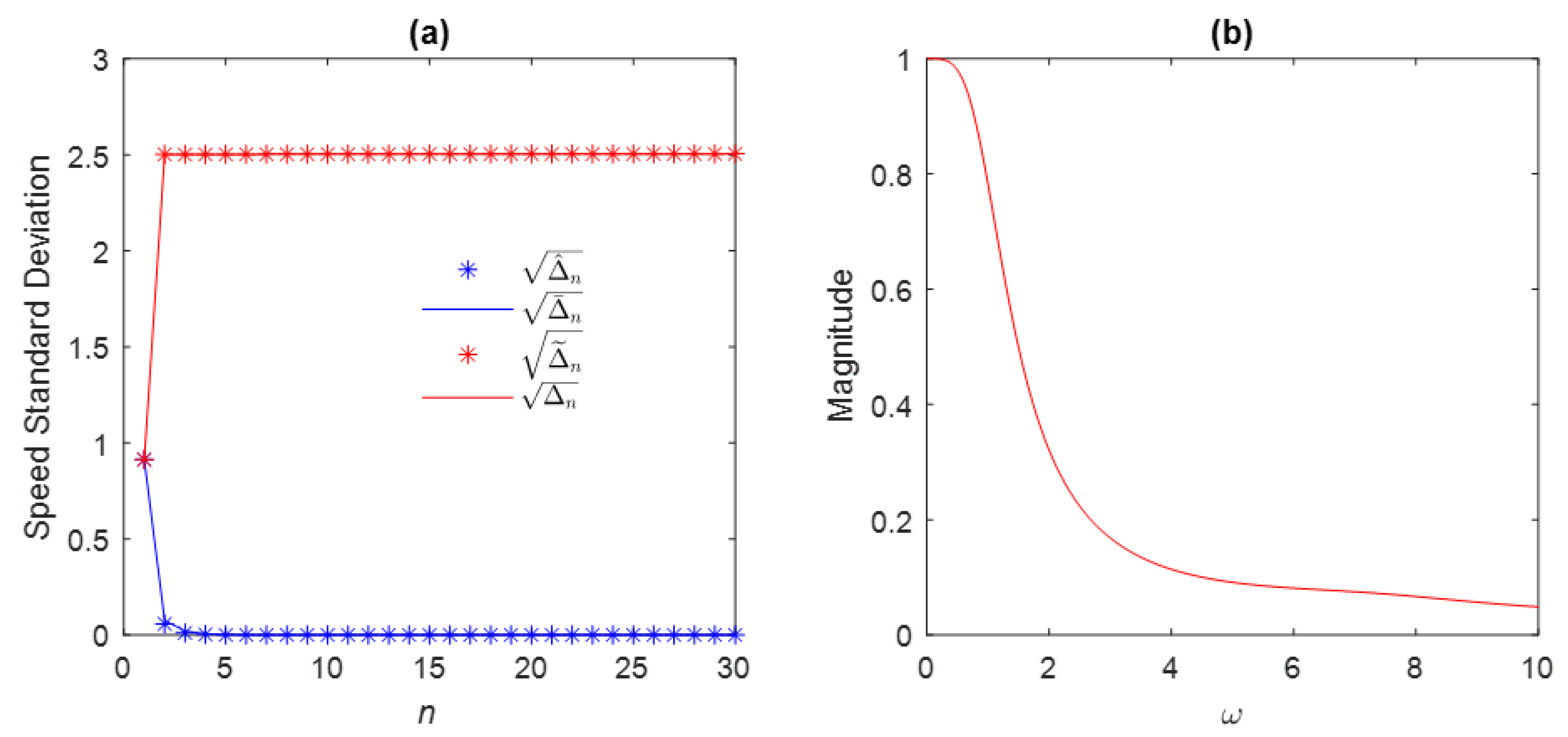
where $\delta$ is the discretization time interval and $d\delta >0$ is vehicle $n$’s reaction time $\tau$. Figure 2 shows the relationship between $\omega$ and $G\left(\omega \right)$ under the Continuous model, as well as $\omega /\delta$ and $\overline{G}\left(\omega \right)$ under the Discrete model. The parameters are as follows: $\alpha =0.5\tau =1.2d=\tau /\delta .$ One can see that $\overline{G}\left(\omega \right)\to G\left(\omega \right)$ as $\delta \to 0$.

We also compare the noise term ${\acute{\Delta }}_n=\frac{{\sigma }^2}{\mathbb{F}}{\int }_0^{\mathbb{F}}\frac{\left(1-{\left|G\left(\omega \right)\right|}^{2\left(n-1\right)}\right)·{\left|H\left(\omega \right)\right|}^2}{\left(1-{\left|G\left(\omega \right)\right|}^2\right)}d\omega$ (Continuous model) with ${\stackrel{`}{\Delta }}_n=\frac{{\sigma }^2}{2\pi }{\int }_0^{2\pi }\frac{\left(1-{\left|G\left(\omega \right)\right|}^{2\left(n-1\right)}\right)}{{\left|L_1\left(\omega \right)\right|}^2\left(1-{\left|G\left(\omega \right)\right|}^2\right)}d\omega$ (Discrete model) in Figure 3. Parameters are as follows: $\mathbb{F}=10$, 100, 1000; ${\sigma }^2=1;\delta =0.1,0.01,0.001;\alpha =0.3\tau =1.4$. One can see that ${\acute{\Delta }}_n\to {\stackrel{`}{\Delta }}_n$ as $\mathbb{F}\to \infty$ and $\delta \to 0$.

In this section, we simulatively show that when a discrete interval δ→0, the transfer function of discrete model converges to that of the continuous model and furthermore, when frequency $\mathbb{F}$→∞, the noise term of discrete function and continuous function converge to each other. Thus, we can derive that ${\Delta }_{n,discrete}\to {\Delta }_n$ when $\mathbb{F}\to \infty$ and $\delta \to 0$. (Simulation shows in Appendix A)

4. Numerical Simulations

In this section, we let the leading vehicle move as $v_1\left(t\right)=A_1\sin \left({\omega }_{1}t\right)+A_2\sin \left({\omega }_{2}t\right),({\omega }_1\ne {\omega }_2)$, then a speed variance of DFM and SFM can be driven through Equations (44) and (46):

$${\overline{\Delta }}_n=\frac{A_1^2}{2}{\left|G\left(\frac{\alpha }{j{\omega }_1{e}^{\tau j{\omega }_1}+\alpha }\right)\right|}^{2\left(n-1\right)}+\frac{A_2^2}{2}{\left|G\left(\frac{\alpha }{j{\omega }_2{e}^{\tau j{\omega }_2}+\alpha }\right)\right|}^{2\left(n-1\right)}$$

(52)

$${\Delta }_n={\overline{\Delta }}_n+\frac{{\sigma }_n^2}{\mathbb{F}}{{\displaystyle \int }}_0^{\mathbb{F}}{\displaystyle \sum }_{m=2}^n{\left|\frac{\alpha }{j\omega e^{\tau j\omega }+\alpha }\right|}^{2\left(n-m\right)}·{\left|\frac{j\omega }{j\omega e^{\tau j\omega }+{\alpha }_n}\right|}^{2}d\omega$$

(53)

To verify Proposition 1, we decompose $v_1\left(t\right)=v_{1,1}\left(t\right)+v_{2,1}\left(t\right)$, where $v_{1,1}\left(t\right)=A_1\sin \left({\omega }_{1}t\right)$ and $v_{2,1}\left(t\right)=A_2\sin \left({\omega }_{2}t\right)$, and we denote the simulation result of speed variance with the leading speed $v_{1,1}\left(t\right)$ and $v_{2,1}\left(t\right)$ under DFM as ${\widehat{\Delta }}_{1,n}$ and ${\widehat{\Delta }}_{2,n}$. We use Equation (46) as the discrete model, $\delta$ = 0.001 as a very tiny discrete time interval to simulate the traffic flow system and ${\widehat{\Delta }}_n≔{\sum }_{i=1+I/5}^I{\left(v_n\left[i\right]\right)}^2$ to denote the simulation speed variance under DFM to avoid the impact of start-up, where $I={10}^6$. Correspondingly, we run the simulation for $M=1000$ iterations under SFM, and directly measure the speed variance of SFM using the following equation:

$${\tilde{\Delta }}_n≔\frac{{{\displaystyle \sum }}_{m=1}^M{{\displaystyle \sum }}_{i=1+\mathrm{I}/5}^I{\left(v_n\left[i\right]\right)}^2}{4MI/5}$$

(54)

The simulation settings are taken as follows: $\mathbb{F}=3000, N=30, \tau =1, d=\tau /\delta , \alpha =0.5, \sigma =2, A_1=1.5, {\omega }_1=1, A_2=1, {\omega }_2=2$. As the results demonstrate in Figure 4, we can see $G\left({\omega }_1\right)<1$ and $G\left({\omega }_2\right)<1$ from Figure 4b, thus DFM with a leading speed of $v_1\left(t\right)$ is stable. We can see that $\sqrt{{\widehat{\Delta }}_{1,n}+{\widehat{\Delta }}_{2,n}},\sqrt{{\overline{\Delta }}_n}$ and $\sqrt{{\widehat{\Delta }}_n}$ overlapped very well with each other, which is consistent with Proposition 1. Additionally, ${\left|G\left(\omega \right)\right|}_{\infty }<1$, thus$\sqrt{{\Delta }_n}\to 2$, is consistent with Proposition 2.

Then, we exam this case with $\tau =1.5$. The simulation result is shown in Figure 5. It is obvious that ${\left|G\left(\omega \right)\right|}_{\infty }>1$ from Figure 5b, thus${\Delta }_n\to \infty$ as$n\to \infty$, which is consistent with Proposition 2.

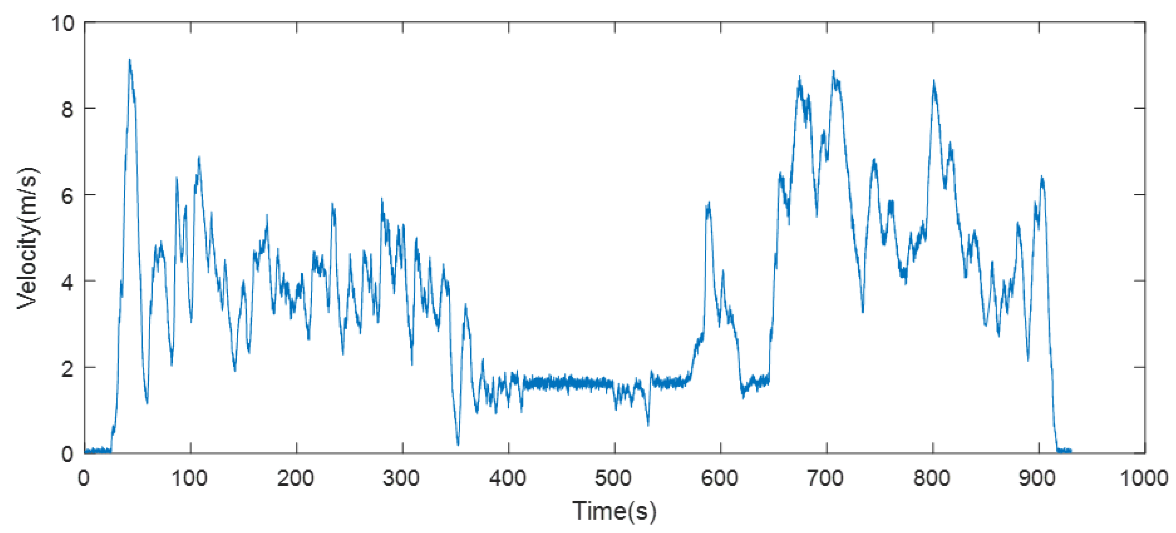
To better correlate with field data, the GPS data from our previous work were utilized [33]. The sampling frequency of the GPS data is 0.1s. We randomly selected the speed track of one vehicle as the speed data of the leading vehicle. The data length is 930.7s, which means T = 9307 sampling points, see Figure 6.

We decompose $v_1\left[i\right]$ as $v_1\left[i\right]={{\displaystyle \sum }}_{k=1}^T{a}_k\sin \left[\frac{k}{T}2\pi i\right]+b_k\cos \left[\frac{k}{T}2\pi i\right]$, where $a_k=\frac{1}{T}{{\displaystyle \sum }}_{i=1}^{T}v\left[i\right]\cos \left(\frac{k}{T}2\pi i\right)$, $b_k=\frac{1}{T}{{\displaystyle \sum }}_{i=1}^{T}v\left[i\right]\sin \left(\frac{k}{T}2\pi i\right)$ and T = 9307. Then, we recompose $v_1\left(t\right)={{\displaystyle \sum }}_{k=1}^T{a}_k\sin \left[\frac{k}{T}2\pi t\right]+b_k\cos \left[\frac{k}{T}2\pi t\right]$ as the leading vehicle. To avoid the impact of start-ups, we used two cycles of the leading vehicle in the simulation. The simulation settings are as follows: $\mathbb{F}=3000, \delta =0.001, N=30, \tau =1, \alpha =0.5, \sigma =2.5$. The simulation result is shown in Figure 7, where the simulation results and the theoretical results overlap with each other and $\sqrt{{\Delta }_n}\to 2.5$, which is consistent with Proposition 2.

5. Conclusions

In this paper, we extend the previous work [30] to the Fist-order continuous model, which allows us to analytically quantify the speed variance without discretize the model, the main contribution of this paper is as follows:

-

This paper presents an analytical expression for the evolution of speed standard deviation under a continuous first-order model.

-

We simulatively show that when the discrete interval δ→0, the transfer function of the discrete model and continuous model converge to each other; when frequency F→∞, the noise term of discrete function and continuous function converge to each other.

-

This paper put forward another view that traffic oscillations are caused not by the model or heterogeneous behavior, but by the disturbance of the drivers/vehicles. From the traffic control aspect, this paper reveals that the key point of dampening the highway traffic oscillations is to reduce the noise caused by driver/vehicles. (Specific measures can be to improve driving concentration, pavement repair, and reduce roadside distractions, etc.)

This study proposed an analytical method for the first-order continuous stochastic model, but there is still work that needs to be done. Firstly, white noise may not be the best choice of the stochastic term; therefore, we need to further analyze the form of noise. Secondly, we need to study the relationship between acceleration noise and velocity noise to extend the method to models such as the optimal velocity model or full velocity difference model. Finally, this method might be potentially extended to nonlinear stochastic models using the describing function method proposed in Li [34].

References

- Pipes, L.A. An operational analysis of traffic dynamics. J. Appl. Phys. 1953, 24, 274–281. [Google Scholar] [CrossRef]
- Newell, G.F. Nonlinear Effects in the Dynamics of Car-following. Oper. Res. 1961, 9, 209–229. [Google Scholar] [CrossRef]
- Bando, M.; Hasebe, K.; Nakayama, A.; Shibata, A.; Sugiyama, Y. Dynamical model of traffic congestion and numerical simulation. Phys. Rev. E 1995, 51, 1035–1042. [Google Scholar] [CrossRef] [PubMed]
- Helbing, D.; Tilch, B. Generalized Force Model of Traffic Dynamics. Phys. Rev. E 1998, 58, 133–138. [Google Scholar] [CrossRef] [Green Version]
- Jiang, R.; Wu, Q.; Zhu, Z. Full velocity difference model for a car-following theory. Phys. Rev. E 2001, 64, 017101. [Google Scholar] [CrossRef] [Green Version]
- Yu, X. Analysis of the stability and density waves for traffic flow. Chin. Phys. 2002, 11, 1128. [Google Scholar] [CrossRef]
- Zhao, X.; Gao, Z. The stability analysis of the full velocity and acceleration velocity model. Phys. A Stat. Mech. Appl. 2007, 375, 679–686. [Google Scholar] [CrossRef]
- Nagatani, T. Stabilization and enhancement of traffic flow by the next-nearest-neighbor interaction. Phys. Rev. E. 1999, 60, 6395–6401. [Google Scholar] [CrossRef] [Green Version]
- Nagatani, T. The physics of traffic jams. Rep. Prog. Phys. 2002, 65, 1331. [Google Scholar] [CrossRef] [Green Version]
- Nagatani, T. Traffic states and fundamental diagram in cellular automaton model of vehicular traffic controlled by signals. Phys. A Stat. Mech. Appl. 2009, 388, 1673–1681. [Google Scholar] [CrossRef]
- Sawada, S. Generalized Optimal Velocity Model for Traffic Flow. Comput. Phys. Commun. 2002, 13, 1–12. [Google Scholar] [CrossRef] [Green Version]
- Jiang, R.; Hu, M.B.; Zhang, H.M.; Gao, Z.Y.; Jia, B.; Wu, Q.S.; Wang, B.; Yang, M. Traffic experiment reveals the nature of car-following. PLoS ONE 2014, 9, e94351. [Google Scholar] [CrossRef] [PubMed] [Green Version]
- Lang, L.; Guo, N.; Jiang, R.; Zhu, K. An improved inertia model to reproduce car-following instability. Phys. A Stat. Mech. Appl. 2019, 526, 121087. [Google Scholar] [CrossRef]
- Xu, T.; Laval, J.A. Analysis of a two-regime stochastic car-following model: Explaining capacity drop and oscillation instabilities. Transp. Res. Rec. 2019, 2673, 610–619. [Google Scholar] [CrossRef]
- Ngoduy, D.; Lee, S.; Treiber, M.; Keyvan-Ekbatani, M.; Vu, H.L. Langevin method for a continuous stochastic car-following model and its stability conditions. Transp. Res. Part C Emerg. Technol. 2019, 105, 599–610. [Google Scholar] [CrossRef] [Green Version]
- Hwang, T.; Ouyang, Y. Urban freight truck routing under stochastic congestion and emission considerations. Sustainability 2015, 7, 6610–6625. [Google Scholar] [CrossRef] [Green Version]
- Jamal, A.; Rahman, M.T.; Al-Ahmadi, H.M.; Ullah, I.; Zahid, M. Intelligent intersection control for delay optimization: Using meta-heuristic search algorithms. Sustainability 2020, 12, 1896. [Google Scholar] [CrossRef] [Green Version]
- Al-Turki, M.; Jamal, A.; Al-Ahmadi, H.M.; Al-Sughaiyer, M.A.; Zahid, M. On the potential impacts of smart traffic control for delay, fuel energy consumption, and emissions: An NSGA-II-based optimization case study from Dhahran, Saudi Arabia. Sustainability 2020, 12, 7394. [Google Scholar] [CrossRef]
- Laval, J.A. Linking synchronized flow and kinematic waves. In Traffic and Granular Flow ’05; Springer Science & Business Media: Berlin/Heidelberg, Germany, 2007. [Google Scholar] [CrossRef]
- Laval, J.A. Lane-changing in traffic streams. Transp. Res. Part B Methodol. 2006, 40, 251–264. [Google Scholar] [CrossRef]
- Zheng, Z.; Ahn, S.; Chen, D.; Laval, J. Applications of wavelet transform for analysis of freeway traffic: Bottlenecks, transient traffic, and traffic oscillations. Transp. Res. Part B Methodol. 2011, 45, 372–384. [Google Scholar] [CrossRef] [Green Version]
- Coifman, B.; Kim, S. Extended bottlenecks, the fundamental relationship, and capacity drop on freeways. Procedia Soc. Behav. Sci. 2011, 17, 44–57. [Google Scholar] [CrossRef] [Green Version]
- Sugiyamal, Y.; Fukui, M.; Kikuchi, M.; Hasebe, K.; Nakayama, A.; Nishinari, K.; Tadaki, S.I.; Yukawa, S. Traffic jams without bottlenecks-experimental evidence for the physical mechanism of the formation of a jam. New J. Phys. 2008, 10, 033001. [Google Scholar] [CrossRef]
- Treiber, M.; Hennecke, A.; Helbing, D. Derivation, Properties, and Simulation of a Gas-Kinetic-Based, Non-Local Traffic Model. Phys. Rev. E 1999, 59, 239–253. [Google Scholar] [CrossRef] [Green Version]
- Treiber, M.; Kesting, A. Validation of traffic flow models with respect to the spatiotemporal evolution of congested traffic patterns. Transp. Res. Part C Emerg. Technol. 2012, 21, 31–41. [Google Scholar] [CrossRef]
- Wilson, R.E.; Ward, J.A. Car-following models: Fifty years of linear stability analysis—A mathematical perspective. Transp. Plan. Technol. 2011, 34, 3–18. [Google Scholar] [CrossRef]
- Laval, J.A.; Leclercq, L. A mechanism to describe the formation and propagation of stop-and-go waves in congested freeway traffic. Philos. Trans. R. Soc. A Math. Phys. Eng. Sci. 2010, 368, 4519–4541. [Google Scholar] [CrossRef] [PubMed] [Green Version]
- Chen, D.; Laval, J.; Zheng, Z.; Ahn, S. A behavioral car-following model that captures traffic oscillations. Transp. Res. Part B Methodol. 2012, 46, 744–761. [Google Scholar] [CrossRef] [Green Version]
- Chen, D.; Laval, J.A.; Ahn, S.; Zheng, Z. Microscopic traffic hysteresis in traffic oscillations: A behavioral perspective. Transp. Res. Part B Methodol. 2012, 46, 1440–1453. [Google Scholar] [CrossRef] [Green Version]
- Wang, Y.; Li, X.; Tian, J.; Jiang, R. Stability analysis of stochastic linear car-following models. Transp. Sci. 2020, 54, 274–297. [Google Scholar] [CrossRef]
- Chu, K.-c. Decentralized Control of High-Speed Vehicular Strings. Transp. Sci. 1974, 8, 361–384. [Google Scholar] [CrossRef]
- Cohen, L. The generalization of the Wiener-Khinchin theorem. In Proceedings of the 1998 IEEE International Conference on Acoustics, Speech and Signal Processing, ICASSP ’98, Seattle, WA, USA, 15 May 1998; Volume 3, pp. 1577–1580. [Google Scholar] [CrossRef]
- Jiang, R.; Jin, C.-J.; Zhang, H.M.; Huang, Y.-X.; Tian, J.-F.; Wang, W.; Hu, M.-B.; Wang, H.; Jia, B. Experimental and Empirical Investigations of Traffic Flow Instability. Transp. Res. Procedia 2017, 23, 157–173. [Google Scholar] [CrossRef]
- Li, X.; Ouyang, Y. Characterization of traffic oscillation propagation under nonlinear car-following laws. Procedia Soc. Behav. Sci. 2011, 17, 663–682. [Google Scholar] [CrossRef] [Green Version]
Figure 1.
Illustration of the car-following system with N vehicles in the system.
Figure 2.
Magnitudes of G(ω) and .
Figure 3.
Noise term comparing between continuous and discrete model.
Figure 4.
Simulation results with : (a) Time-Domain Speed Standard Deviation; (b) Magnitudes of , and .
Figure 5.
Figure 6.
Leading vehicle speed data.
Figure 7.
Simulation results with : (a) Time-Domain Speed Standard Deviation; (b) Magnitudes of .