Modeling Multistep Ahead Dissolved Oxygen Concentration Using Improved Support Vector Machines by a Hybrid Metaheuristic Algorithm

Abstract

Dissolved oxygen (DO) concentration is an important water-quality parameter, and its estimation is very important for aquatic ecosystems, drinking water resources, and agro-industrial activities. In the presented study, a new support vector machine (SVM) method, which is improved by hybrid firefly algorithm–particle swarm optimization (FFAPSO), is proposed for the accurate estimation of the DO. Daily pH, temperature (T), electrical conductivity (EC), river discharge (Q) and DO data from Fountain Creek near Fountain, the United States, were used for the model development. Various combinations of pH, T, EC, and Q were used as inputs to the models to estimate the DO. The outcomes of the proposed SVM–FFAPSO model were compared with the SVM–PSO, SVM–FFA, and standalone SVM with respect to the root mean square errors (RMSE), the mean absolute error (MAE), Nash–Sutcliffe efficiency (NSE), and determination coefficient (R²), and graphical methods, such as scatterplots, and Taylor and violin charts. The SVM–FFAPSO showed a superior performance to the other methods in the estimation of the DO. The best model of each method was also assessed in multistep-ahead (from 1- to 7-day ahead) DO, and the superiority of the proposed method was observed from the comparison. The general outcomes recommend the use of SVM–FFAPSO in DO modeling, and this method can be useful for decision-makers in urban water planning and management.

1. Introduction

Nowadays, the control of freshwater quality is a strategic priority for water resource and management [1], and for a better reduction in water pollution [2]. The dissolved oxygen concentration is an important water quality variable, and its fluctuation in response to several chemical, biochemical, and physical factors has been well documented [3]. Currently, in situ measurements of DO concentrations, which are often accompanied by other water quality variables, have facilitated the development and application of a large number of numerical models for the better prediction of the DO in freshwater ecosystems. Because of the effect of other variables, the DO modeling becomes nonlinear in nature, and it is difficult to capture nonlinearity with simple models. However, models that are based on machine learning (ML) are the most widely used for modeling nonlinear variables, and they have gained much popularity during the last few years [4,5,6,7]. In practice, the calculated DO using numerical models has its own error. Thus, the research is heavily oriented towards the development of algorithms that reduce the prediction errors and that help in obtaining adequate predictive accuracies. In some case, the wrong selection of the model’s parameters and the inadequate models’ calibrations following poor model training significantly inflate the overall modeling error that is calculated between the measured and the predicted data [8]. Ultimately, in order to reduce the prediction errors and to improve the ML model performances, various attempts have been made by utilizing algorithms that are capable of making better selections of the models’ parameters [9,10]. These algorithms can be classified into two categories: (i) Algorithms that improve the models’ performances by maximizing the contribution of the input variables, which is achieved by using preprocessing signal decomposition (PSD) algorithms (i.e., wavelet transform and empirical mode decomposition, among others [11,12]), and (ii) Algorithms that improve the generalization capabilities of the ML models by the correct choice of model parameters, which is generally achieved by using metaheuristic optimization algorithms (MOAs) (i.e., genetic algorithms, and particle swarm optimization (PSO)). While the use of PSD has gained much popularity, especially for solving problems that are based on long datasets, the number of developed algorithms is very limited compared to MOAs, for which their increased use has attracted the attention of researcher’s worldwide, and the number of developed algorithms is provided in an always increasing way [13].

Until now, the modeling of dissolved oxygen has included single and hybrid models. In general, modeling using single models was formulated as an approximation function that involves the inclusion of specific water-quality variables, while accepting the need to select easily measured variables. While recognizing that this modeling strategy has the advantage of having a simple and direct mathematical formulation, the poor generalization capabilities, in some cases, and the extensive research to determine the best model parameters using a hard trial-and-error process, alternative approaches that are based on model optimization using MOAs, can be seen as complementary alternative approaches that lead to the better selection of the model parameters. The literature review reveals that several single models for DO prediction are available in the literature, such as: the long short-term memory (LSTM) deep neural network model [14,15]; deterministic models (i.e., MINLAKE2018) [16]; the linear dynamic system and filtering model [17]; the gated recurrent unit (GRU) deep neural network model [18]; support vector regression (SVR) [19]; the stochastic vector auto regression (SVAR) model [20]; the radial basis function neural network (RBFNN) [21]; the multilayer perceptron neural network (MLPNN) [22]; polynomial chaos expansions (PCE) [23]; random forest regression (RFR) [24]; the extremely randomized tree [25]; and multivariate adaptive regression splines (MARS) [26].

Several hybrid models that use MOAs for DO prediction have been proposed over the last few years. Yang et al. [27] investigated the capabilities and robustness of new hybrid models that were applied for predicting the daily DO in the Klamath River, Oregon, the United States. They hybridized the MLPNN model by using three MOAs, namely, the multi-verse optimizer (MVO), the black hole algorithm (BHA), and shuffled complex evolution (SCE), were developed and compared: (i) The MVO–MLPNN; (ii) The BHA-MLPNN; and (iii) The SCE–MLPNN. The three models were calibrated by using three water-quality variables, namely, the water temperature (T_w), the pH, and the specific conductance (SC). According to the obtained results, the SCE–MLPNN was more accurate, and it exhibited a high correlation coefficient (R ≈ 0.877), compared to the values of (R ≈ 0.845) and (R ≈ 0.874) that were obtained using the MVO–MLPNN and the BHA–MLPNN, respectively. In a recently conducted investigation, Zhu et al. [28] used four MOAs for optimizing the least squares support vector regression (LSSVR) model. The MOAs that were used were as follows: the fruit fly optimization algorithm (FFA); the particle swarm optimization (PSO) algorithm; the genetic algorithm (GA); and the immune genetic algorithm (IGA). Hence, four hybrid models were proposed: (i) FFA–LSSVR; (ii) PSO–LSSVR; (iii) GA-LSSVR; and (iv) IGA-LSSVR. Numerical comparison between models revealed that the FFA-LSSVR exhibited high predictive accuracies compared to the PSO–LSSVR, GA-LSSVR, and IGA-LSSVR for which the mean absolute percentage errors were ≈0.35%, ≈1.3%, ≈2.03% and ≈1.33%, respectively. Raheli et al. [29] compared between hybrid FFA-MLPNN and single MLPNN in predicting monthly DO concentration in the Langat River, Malaysia. Comparison between the hybrid and single models revealed the superiority of the FFA-MLPNN (R ≈ 0.820, root mean square error, RMSE ≈ 0.497%) compared to the values obtained using the single MLPNN (R ≈ 0.727, RMSE ≈ 0.606). In another study, Deng et al. [30] used the PSO algorithm combined with the MLPNN for developing a hybrid PSO-MLPNN model, which was used for predicting DO concentration in an aquiculture pond, showing the superiority of the PSO-MLPNN compared to the single MLPNN without providing numerical comparison. Song et al. [31] proposed a new hybrid MOA called the improved sparrow search algorithm (ISSA) coupled LSTM (ISSA-LSTM) for predicting weekly DO concentration in the Haihe River, China. The performances of the ISSA-LSTM were compared to those of (SSA-LSTM), gray wolf optimization algorithm (GWO) coupled LSTM (GWO-LSTM), and the whale optimization algorithm (WOA) coupled LSTM (WOA-LSTM). A comparison of the models’ overall performances revealed that the ISSA-LSTM was more accurate, exhibiting the high predictive accuracies and the greatest improvement in terms of mean absolute error (MAE) and RMSE, compared to the standard LSTM, for which the decrease rate was ≈30.47% (SSA–LSTM), ≈36.22% (ISSA–LSTM), ≈21.34% (GWO–LSTM) and ≈19.08% (WOA–LSTM) in terms of MAE, and ≈34.98% (SSA–LSTM), ≈37.27% (ISSA–LSTM), ≈19.53% (GWO–LSTM) and ≈17.88% (WOA–LSTM) in terms of RMSE, respectively. From the obtained results, it is clear that the ISSA–LSTM was the most accurate and the GWO–LSTM was the poorest model.

A hybrid model combining the fractional grey seasonal model and the PSO algorithm (PSO–FGSM) was proposed in [32]. The accuracies of the PSO–FGSM were compared to those of the Holt–Winters model optimized using GWO (GWO–HW). These two hybrid models were applied and compared for forecasting monthly DO concentration in the Huaihe River, China. The outcomes showed the superiority of the PSO–FGSM, which had a MAPE ranging from ≈8.66% to ≈10.73%, compared to the values obtained using the GWO–HW, i.e., MAPE ranging from ≈10.29% to ≈13.20%. Cao et al. [33] used the PSO algorithm for optimizing the softplus extreme learning machine (SELM), and they applied the hybrid PSO–SELM for predicting DO concentration. According to the obtained results, the PSO–SELM was more accurate and provided the best predictive accuracies with Nash–Sutcliffe efficiency (NSE), RMSE and MAE equal to ≈0.952, ≈0.270 and ≈0.228 compared to the values obtained using ELM (NSE ≈ 0.908, RMSE ≈ 0.377, MAE ≈ 0.333), MLPNN (NSE ≈ 0.903, RMSE ≈ 0.390, MAE ≈ 0.322), LSTM (NSE ≈ 0.887, RMSE ≈ 0.416, MAE ≈ 0.336), and SVR (NSE ≈ 0.859, RMSE ≈ 0.466, MAE ≈ 0.391), respectively. Dehghani et al. [34] employed the SVR model combined with four MOA algorithms namely: (i) the algorithm of the innovative gunner (AIG), (ii) the black widow optimization (BWO), (iii) social skidriver (SSD) optimization, and (iv) the chicken swarm optimization (CSO). The four hybrid models, i.e., AIG–SVR, BWO–SVR, SSD–SVR, and CSO–SVR were applied for predicting monthly DO concentration in the Cumberland River, USA, using water temperature (T_w) and river discharge (Q). According to the obtained results, the best prediction accuracies were obtained using the AIG–SVR (R ≈ 0.963, NSE ≈ 0.864, RMSE ≈ 0.644, and MAE ≈ 0.568). It was also found that the hybrid models improved the accuracies of the single SVR by 1.5% to 6.5%. Several other hybrid models for DO concentration can be found in the literature, for example, MLPNN optimized genetic algorithm (GA–MLPNN) [35], gene expression programming with PSO (PSO–GEP) [36], and differential evolution (DE) optimized radial basis function (DE–RBFNN) [37].

Jiang et al. [38] applied the wavelet–Lyapunov exponent model (WLME) for forecasting DO concentration at weekly and 15 min intervals. The proposed WLME is the result of a combination of the wavelet decomposition, chaos theory and Lyapunov exponent’s models. It was found that the WLME was more accurate compared to the standalone MLPNN and the autoregressive moving average (ARMA) exhibits an average relative error (ARE) of 2.35%. Huang et al. [39] introduced a hybrid model composed of deep auto–regression recurrent neural network (DeepAR) and the variational mode decomposition (VMD), which are used as a preprocessing signal decomposition. In addition, the sparrow swarm algorithm (SSA) was used for model parameters’ optimization. The hybrid model, i.e., VMD-DeepAR-SSA, was compared to the standalone Bayesian and Bootstrap and it exhibited a prediction interval coverage probability (PICP) of 0.950. Li et al. [40] proposed the hybrid models by combining the LSTM and the temporal convolutional network (TCN), i.e., the LSTM-TCN, for predicting DO concentration, and reported its high performances with MAE, RMSE, and R² of 0.236, 0.342 and 0.94, respectively. Yang and Liu [41] adopted the complete ensemble empirical mode decomposition with adaptive noise (CEEMDAN) as preprocessing signal decomposition for decomposing water quality variables, which are used as inputs for the LSTM model applied for predicting DO concentration. They carried out an analysis looking at comparative performances between the proposed CEEMDAN–LSTM and, respectively, the RBFNN, the recurrent neural network (RNN), GRU, CEEMDAN–RBFNN, CEEMDAN–RNN, CEEMDAN–GRU, VMD–LSTM, and wavelet transform LSTM (WT–LSTM). Obtained results revealed that the best prediction accuracies were obtained using the CEEMDAN–LSTM with MAE, RMSE, and MAPE of 0.102, 0.121 and 0.0149, respectively. Moghadam et al. [42] compared deep recurrent neural network (DRNN), the SVM and the MLPNN models for predicting DO at (t + 1), (t + 3) and (t + 7) time=horizons. It was found that the DRNN was more accurate compared to the other models and the forecasting accuracies decreased by increasing the forecasting horizon. Song and Yao [43] introduced a new modeling framework for better prediction of DO concentration by combining three different paradigms, namely deep extreme learning machine (DELM), synchro-squeezed wavelet transform and sparrow search algorithm (SSA), i.e., the SWT–SSA–DELM. Results obtained using the proposed model was compared to those obtained using ELM, SWT–ELM, SSA–ELM, SWT–SSA–ELM, DELM, SWT–DELM, SSA–DELM, and finally SWT–SSA–DELM. It was found that the SWT–SSA–DELM was more accurate exhibiting very low MAE (≈0.131) and RMSE (≈0.171) and very high R (≈0.982) and NSE (≈0.965) values. Recently, a hybrid model based on extreme gradient boosting (XGBoost), improved sparrow search algorithm (ISSA) and LSTM model, i.e., the XGBoost-ISSA–LSTM was proposed by Wu et al. [44] for multi steps ahead forecasting of DO concentration. It was found that, in one hand, high forecasting accuracies can be obtained and in the other hand, the performance of the model decreased by increasing the forecasting horizon. In addition, a comparative study among several other hybrid models revealed that the XGBoost-ISSA-LSTM was more accurate compared to XGBoost-RFR, XGBoost-MLPNN, XGBoost-RNN, XGBoost-GRU, LSTM, XGBoost-LSTM, XGBoost-PSO-LSTM, and XGBoost-SSA-LSTM.

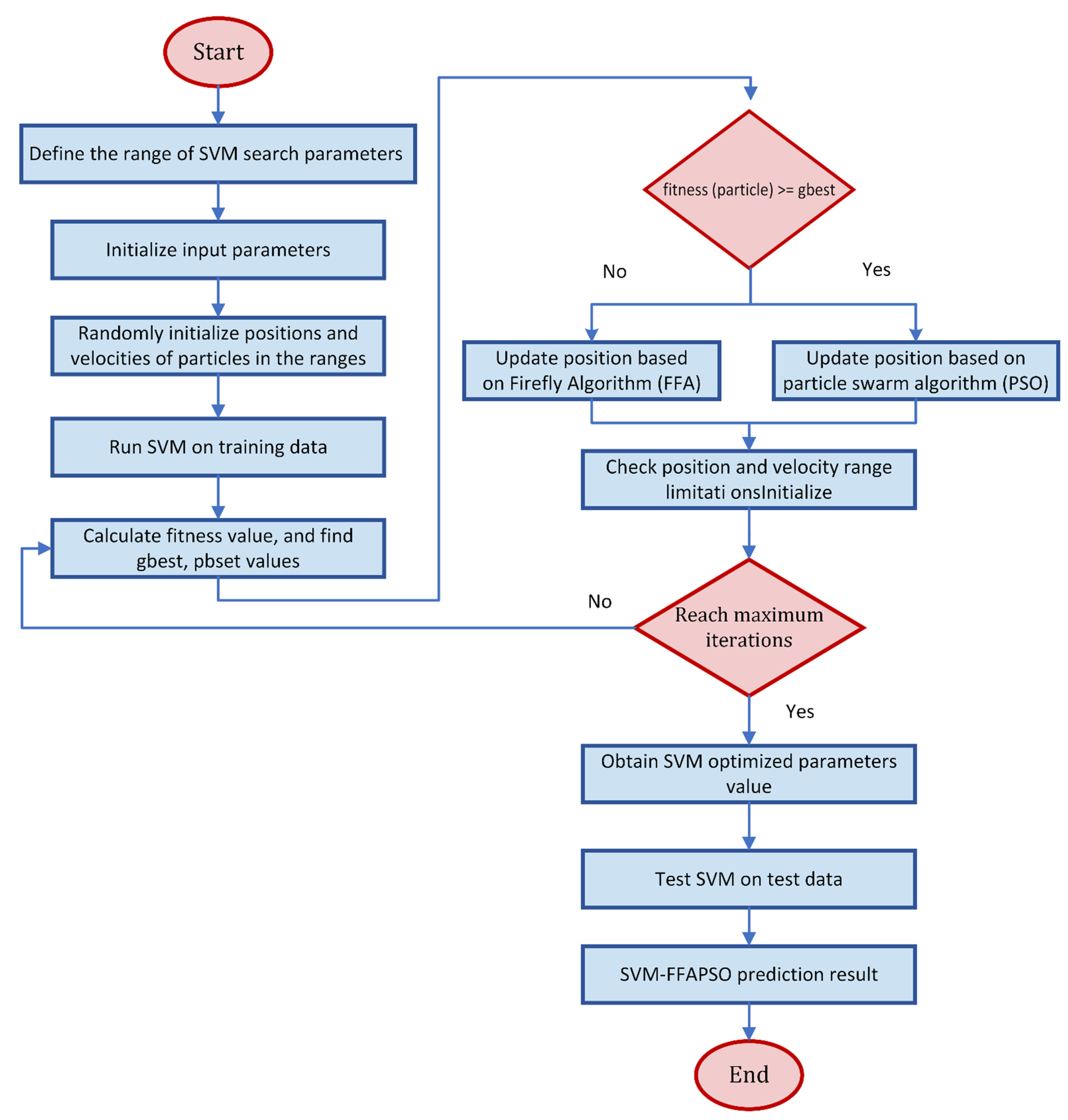
Our motivation is to introduce a new hybrid model for better prediction of DO concentration in rivers, using SVR optimization based on firefly algorithm particle swarm optimization (FFAPSO–SVR). The proposed FFAPSO–SVR was compared to the SVR, FFA–SVR and PSO–SVR, while hybridizing the SVR and LSSVR using MOA was reported in the literature [28,34]. To the best of our knowledge, combining the FFA and PSO to provide a single algorithm coupled with the SVR model has never reported in the literature, therefore constituting the major motivation of our study. 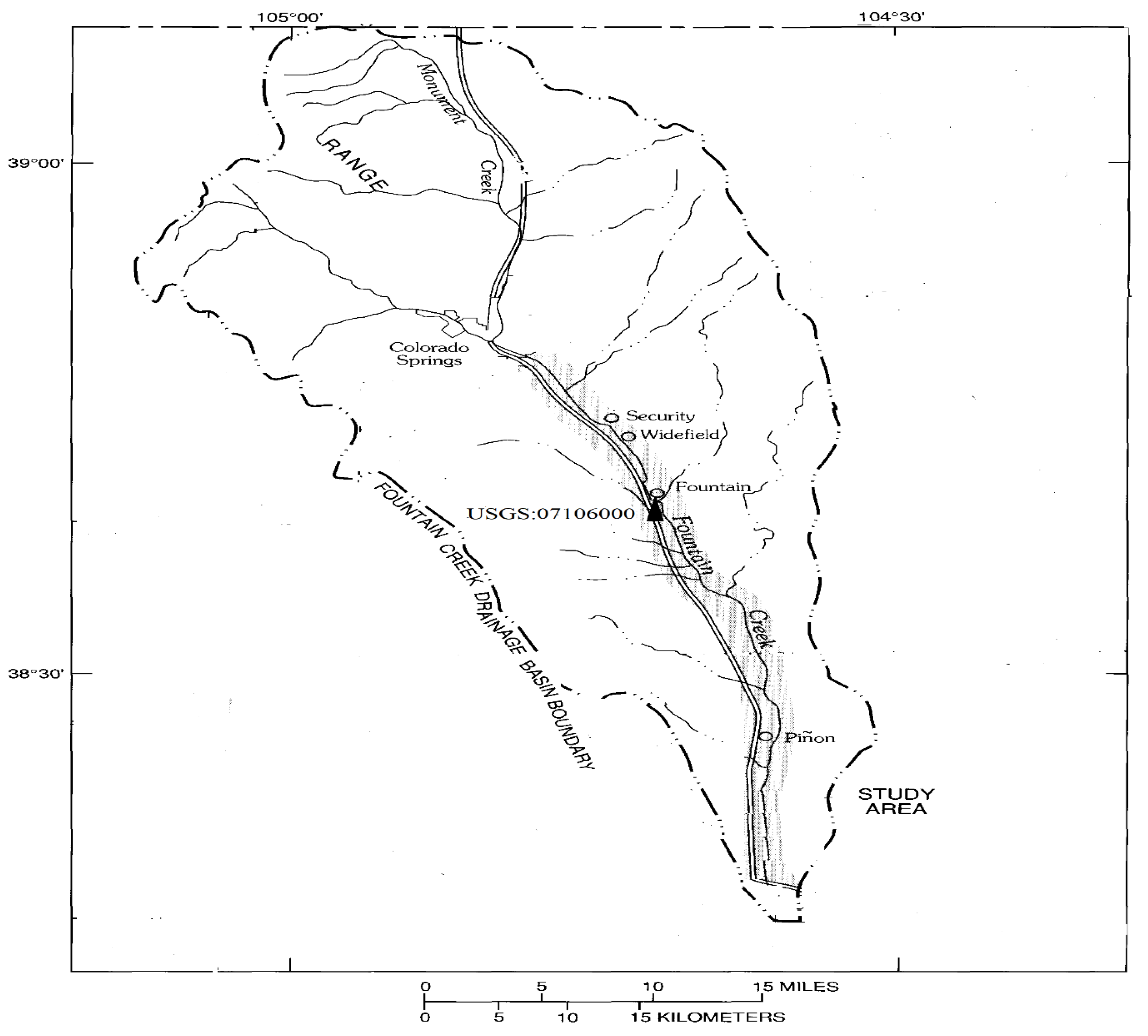The rest of the paper is organized as follows: Section 2 describes the case study and briefly describes each model applied in this study. Section 3 presents the main results and discusses their relevance. Finally, the main conclusions drawn from this study are presented in Section 4.

2. Materials and Methods

2.1. Case Study

The study area is situated in the Fountain Creek basin near Fountain, Colorado, USA, as shown in Figure 1. The study station adopted in this study is operated by USGS with operational id of Station No: 07106000 (38.36° N latitude and 104.40° E longitude). The selected station covers a gross area of 1763.78 km² with gauge datum of 5353 ft. above sea level. This region has a subtropical monsoon climate with large spatial and temporal variability. Dissolved oxygen (DO) plays a vital role in determining the water quality of site. Therefore, the DO of this station was selected to analyze the water quality of this site. To model DO, daily time series data of DO, pH, T, EC and Q were obtained from the website of USGS for the duration of 1 January 1995 to 31 January 2011. So as to improve the modeling procedure and data quality, unrecorded dates of some variables were excluded from the study. Therefore, a total of 4637 sample data points of 5 selected variables (DO, pH, T, EC and Q) was adopted. Out of 4637 sample data points, 80 percent of data (3727) were used as the training dataset for selected machine learning models, while the remaining 20 percent of data (910) were adopted as the testing dataset. For the training dataset, the maximum–minimum values are 13.1–5.8, 24.6–0, 1280–287, 2530–32 and 12.2–5.2 for the pH, T, EC, Q and DO variables, whereas the corresponding values for the testing are 12.7–6.3, 23.1–0, 1290–425, 844–39 and 11.1–5.9, respectively. Standard deviation and skewness values of training datasets are 1.60–0.19, 6.45–0.12, 139.7–1.35, 178.7–5.27 and 1.42–0.21 for the pH, T, EC, Q and DO variables, respectively, while the corresponding statistics are 1.39–0.02, 6.44–0.21, 115.9–1.04, 65.5–4.25 and 1.30–0.06 for the testing datasets, respectively. As can be clearly seen, the Q variable has the highest skewed distribution in both training and testing datasets, followed by the EC data. The pH and DO data are very close to normal distribution.

2.2. Support Vector Machine (SVM)

Model support vector machines (SVM) have been applied in many scientific areas of research in the last decade. This is due to their theoretical and applied benefits, which validate their development, presentation and classification. The major contribution of this model is to find the hyperplane that finely divides the data points, which is vital for determining a decision boundary with an extreme geometric margin. This is applicable to signal processing, pattern recognition, and non-linear regression [45,46,47]. Vladimir Vapnik developed the SVM in 1995 (AT and T Bell Laboratory) to predict future phenomena with statistical learning analysis [45]. SVM is applied to estimate exact non-linear relationships between input and output variables, helping to solve the real-life problems which are based on non-linear classification. The structure of the SVM model is shown in Figure 2.

Consider input vector data as $X=\left\{r_k\right\}\in R^d$ and $Y=\left\{s_k\right\}\in R$ is as output vector data, which are merged to prepare the training data set as $\left\{\left(r_1, s_1\right),\left(r_2, s_2\right), \dots ,\left(r_N, s_N\right) \right\}$ with $s_k\in \left\{-1,+1\right\}$ as for class tags and $Y\left(X\right)=sign\left[w^{T}X+b\right]$ as linear classifier, here N denotes as number of samples. The training data set is divided into two parts, as discussed below:

$$\{\begin{array}{c}{w}^T{r}_k+b\ge +1, if s_k=+1\\ w^T{r}_k+b\le -1, if s_k=-1\end{array}$$

(1)

It can be further written as:

$$Y\left[w^{T}X+b\right]\ge 1$$

The base of the SVM model is the theory of convex optimization; it takes the Lagrangian optimality properties to discover the constrained optimization. The solution of this problem is obtained using dual space of Lagrange multipliers with the following resulting classifier:

$$s\left(r\right)=sign\left[{\displaystyle \sum }_{k=1}^N{\alpha }_k{s}_k{r}_k^{T}r+b\right]$$

(2)

Additionally, in this SVM classifier, additional slack variable is used to formulate the current problem and the following modified set of inequalities are [45]:

$$Y\left[w^{T}X+b\right]\ge 1-\xi , where \xi =\left\{{\xi }_1,{\xi }_2,\dots ,{\xi }_N \right\}$$

This new SVM formulation is used to estimate both linear and non-linear function. For the classical SVM style and least square type of SVM is used to consider the equality kind of constraints [48,49]. To reduce the lengthy task of determining the solutions to complex problems, SVM reformulation is used. The primal space is as,

$$s\left(r\right)=sign\left[w^{T}r+b\right]$$

(3)

Here, b is real constant and the non-linear classification the dual space is of the form,

$$s\left(r\right)=sign\left[{\displaystyle \sum }_{k=1}^N{\alpha }_k{s}_{k}K\left(r,r_k\right)+b\right]$$

(4)

where ${\alpha }_1,{\alpha }_2,\dots ,{\alpha }_N$ are positive real constants, and $b$ is a real constant. In general, $K\left(r,r_k\right)=\langle \phi (r_{k),}\phi \left(r\right)\rangle$, $\langle ·,·\rangle$ is the inner product, and $\phi \left(r\right)$ is the non-linear map from original space to higher-dimensional space. The SVM model for functional estimation takes the form

$$s\left(r\right)={\displaystyle \sum }_{k=1}^N{\alpha }_k{s}_{k}K\left(r,r_k\right)+b$$

(5)

K(r,r_k) is a kernel function satisfying Mercer condition, such as Gaussian, polynomial or sigmoid kernels. It is defined as

$$K\left(r,r_k\right)=\Phi {\left(r\right)}^T\Phi \left(r_k\right)$$

(6)

Here, RBF (radial basis function) has two parameters $\alpha$ and $\gamma$ which are width and regularization constant. Although, the SVM model provides the ultimate results, it has many shortcomings. The main shortcoming is the descriptor’s selection.

2.3. SVM–FFA (Firefly Algorithm)

Biological systems are very much inspired to develop most of the meta-heuristic algorithms, FFA is one of those which is inspired from natural phenomena. This natural algorithm looks for the optimal solution of the problem by modeling the behavior of a set of fireflies and assigning a relevant value corresponding to the location fitness of each firefly as a model for firefly luciferin by updating the location of the fireflies in the successive iterations of the algorithm. The major two phases of this model are light intensity and formulation of attractiveness for each iteration of the updating phase. So, in this section, the fireflies move toward other fireflies with higher light intensity in their neighborhood. That is why the successive iterations provide the set moves towards a better solution [50,51,52].

The major FFA rules are as below:

(a)

Unisex fireflies;

(b)

Increase in attractiveness of the fireflies;

(c)

All fireflies have unique brightness.

The major tasks of the FFA model are brightness and objective function deviation with respect to different distances.

$$I\left(r\right)=I_0{e}^{\left(-\gamma r^2\right)}$$

(7)

here I depicts the brightness at distance r from a firefly, I₀ is starting brightness, $\gamma$ is light absorption. $\beta$ is introduced to represent the next attractiveness at distance r from the firefly and ${\beta }_0$ is attractiveness at distance r = 0 as

$$\beta \left(r\right)={\beta }_0{e}^{\left(-\gamma r^2\right)}$$

(8)

$$r_{ij}=\Vert x_i+x_j\Vert =\sqrt{{\displaystyle \sum _{k=1}^d\left(x_{i,k}-x_{j,k}\right)}}$$

(9)

this $r_{ij}$ is the Cartesian distance between two fireflies i and j and the movement of firefly i as attracted to another brighter firefly j can be represented as below

$$\Delta x_i={\beta }_0{e}^{\left(-\gamma r^2\right)}\left(x_j-x_i\right)+\alpha {\in }_i$$

(10)

The next movement of firefly i is updated as below

$$x_i^{i+1}=x_i+\Delta x_i$$

(11)

The SVM model is used to select the proper parameter for the next iteration of firefly, which helps to determine the optimal SVM parameters. The working flow of the SVM–FFA model is shown in Figure 3.

2.4. SVM–Particle Swarm Optimization (PSO)

Particle swarm optimization (PSO) is a very popular method, inspired by the social behavior of natural living creatures. The method focuses on specific kinds of animals that unequivocally move in groups and share in the experience of other members, for instance, feathered animals racing to a food source. This is related to an advanced look for answers regarding non-direct conditions in a genuine esteemed pursuit space. Kennedy and Eberhart developed this PSO as the new model for global optimization in 1995 [53,54].

In PSO, every particle i has two vectors, namely a velocity vector and a position vector. The apprise process works according to the preceding best position and the entire swarm preceding best position. The particle i adjusts its velocity vector $v_i$ and position vector $x_i$ as per the below given equations:

$$v^{n+1}=\omega v^n+c_1{r}_1\left(p^n-x^n\right)+c_2{r}_2\left(p_g^n-x^n\right)$$

(12)

$$x^{n+1}=x^n+\beta v^n$$

(13)

where $v^n$ and $x^n$ are the present velocity and position of the particle, $r_1$ and $r_2$ are two independently uniformly distributed arbitrary variables with a range, $p^n$ depicts the best preceding position of the particle i, $p_g^n$ shows the best position among all particles in the population.

This algorithm has become very famous in many areas of research in just a few years due to its adaptability to all optimization problems by having a selection of particles that move around a hunt space. An exact answer can be obtained by any particle in the neighborhood. To evaluate the distance between the particles, the Euclidian algorithm is used, which is important for the development of particles’ communication. The topological neighborhoods inconsequential to the area are used for the famous model gbest. Here, swarm is used to acquire the input data. It will be more effective when PSO properties are combined with the SVM model. The basic working flow of the SVM–PSO model is shown in Figure 4 [55,56].

2.5. Proposed New Hybrid Model (Support Vector Machines Tuned with Firefly Algorithm Particle Swarm Optimization (SVR–FFAPSO))

The tuning parameter λ plays a vital role in obtaining the optimal results from the penalized support vector machine with L1-norm. In this process of penalization, λ governs the transaction between the number of selected descriptors and classification. So, it is very important to select a suitable value of λ. If the value is small, then it leads to overfitting the data as the large numbers of descriptors will not be removed. To choose wisely the value of λ, the data-driven cross-validation approach is used in the literature. However, it identifies many irrelevant descriptors as the number of a descriptor is large, it is also time-consuming. To overcome this problem, metaheuristics algorithms play an important role. By using the hybridization, many different metaheuristics algorithms can be clubbed into a single framework, take favors of the used algorithms and then yield a more favorable performance than using a single algorithm. PSO is most widely used, but it requires leaving the local optima to circumvent premature convergence. Additionally, in PSO, the problem becomes more complex as the variable size increases. On the other hand, FFA is a competent local searching methodology but the major drawback of becoming trapped in local minimum is due to the intensity of the light for attraction.

In this study, a new hybrid model named FFAPSO method developed in [57], is utilized. In this new algorithm, FFA is embedded in PSO to make it more powerful by improving the exploration and exploitation of the PSO model. The main steps of the FFAPSO method are demonstrated in [57]. In this section, the hybrid FFAPSO method is used to obtain the optimal values of the SVM parameters (ε, C, and γ). This proposed hybridization is used to find the value of parameters, the L1-norm. The basic working flow of the SVM–FFAPSO model is shown in Figure 5, and summarized in the following steps:

Step 1: Define the range of SVM searching parameters.

Step 2: Generate initial parameter population (set of individuals).

Step 3: Split dataset into two sets (training and testing sets).

Step 4: Train SVM model using k-fold cross validation on training dataset.

Step 5: Calculate the fitness value of each individual in the population according to the root mean square error (RMSE).

Step 6: Find the global best individual (gbest) and local best individual (pbest).

Step 7: Update the position of each individual using FFAPSO as follows: If fitness of the individual $\le$ gbest, update position using FFA algorithm. Otherwise, update position using PSO algorithm.

Step 8: Repeat step 5–7 until reach the maximum number of iterations.

Step 9: Output the optimal set of parameters (gbest) found at the end of the iteration. Then, train the SVM model with these parameters.

Step 10: Predict the output of data in testing dataset part by SVM model.

2.6. Model Performance Evaluation Matrices

The outcomes of the SVM, SVM–PSO, SVM–FFA and SVM–FFAPSO models were assessed by the following comparison criteria:

$$RMSE:Root Mean Square Erro=\frac{1}{N}{\displaystyle \sum }_{i=1}^N{\left[{(D{O}_0)}_i-{(D{O}_C)}_i\right]}^2$$

(14)

$$MAE:Mean Absolute Error=\frac{1}{N}{\displaystyle \sum }_{i=1}^N|{(D{O}_0)}_i-{(D{O}_C)}_i|$$

(15)

$$R^2:Determination Coefficient={\left[\frac{{{\displaystyle \sum }}_{t=1}^N\left(D{O}_0-\overline{D{O}_0}\right)\left(D{O}_c-\overline{D{O}_c}\right)}{\sqrt{{{\displaystyle \sum }}_{t=1}^N{(D{O}_0-\overline{D{O}_0})}^2{(D{O}_c-\overline{D{O}_c})}^2}}\right]}^2$$

(16)

$$NSE:Nash-Suutcliffe=1-\frac{{{\displaystyle \sum }}_{i=1}^N{[{(D{O}_0)}_i-{(D{O}_c)}_i]}^2}{{{\displaystyle \sum }}_{i=1}^N{[{(D{O}_0)}_i-{\overline{DO}}_0]}^2},-\infty <NSE\le 1$$

(17)

where $D{O}_c$ is computed DO, $D{O}_0$ is observed DO, ${\overline{DO}}_0$ is average of the measured or observed DO and, $N$ is data quantity. These indexes are adopted due to their successful usage in the literature [58,59,60,61,62].

3. Application and Results

In the present study, the SVM hyperparameters were tuned by following the suggestion by Sudheer et al. (2014). The parameters $C$, $\gamma$, and $\epsilon$ were searched in the exponential space $C\in \left({10}^{-5},{10}^5\right)$, $\gamma \in \left(0,{10}^1\right)$ and $\epsilon \in \left(0,{10}^1\right)$.

Table 1. Parameter setting of the optimization algorithms used in the study.

SVM	$C$	10
	$\gamma$	0.1
	$\epsilon$	0.01
	Kernel type	Radial basis function (RBF)
PSO	Cognitive component ($c_1$)	1.49445
	Social component ($c_2$)	1.49445
	inertia weight	0.5–0.9
FFA	Initial value of randomization parameter ($\alpha$)	0.5
	Absorption coefficient ($\gamma$)	1.0
FFAPSO	As in both PSO and FFA
All algorithms	Population	25
	Number of iterations	100
	Number of runs for each algorithm	25

sums up brief information about the set parameters for the implemented method and algorithms. Data split rule of 80–20% was used before applying the machine learning methods. Forty populations and 100 iterations were set for all algorithms. They were run 25 times and their averages were recorded. Several combinations of four variables (T, pH, EC and Q) were used as input to the models to estimate daily DO.

Table 2. The comparison of SVM model in DO estimation.

No. of Inputs	Input Combinations	Training				Testing
		RMSE	MAE	R2	NSE	RMSE	MAE	R2	NSE
1	T	0.631	0.456	0.802	0.802	0.360	0.274	0.931	0.923
	pH	0.391	0.311	0.942	0.924	0.331	0.282	0.961	0.935
	EC	1.383	1.177	0.05	0.05	1.302	1.134	0.022	0.009
	Q	1.417	1.206	0.002	0.002	1.296	1.14	0.006	0.004
2	T, pH	0.379	0.297	0.93	0.929	0.362	0.285	0.955	0.922
	T, EC	0.634	0.456	0.801	0.8	0.36	0.275	0.927	0.92
	T, Q	0.647	0.47	0.793	0.792	0.357	0.272	0.931	0.924
	pH, EC	0.356	0.279	0.942	0.937	0.32	0.263	0.965	0.939
	Q, EC	1.372	1.167	0.065	0.065	1.33	1.133	0.078	0.053
	pH, Q	0.394	0.306	0.94	0.923	0.317	0.269	0.961	0.94
3	T, pH, EC	0.326	0.245	0.948	0.947	0.225	0.179	0.97	0.961
	T, pH, Q	0.432	0.336	0.914	0.907	0.366	0.288	0.942	0.92
	T, EC, Q	0.648	0.478	0.792	0.791	0.404	0.32	0.93	0.903
	pH, Q, EC	0.356	0.278	0.942	0.937	0.304	0.234	0.966	0.945
4	T, pH, EC, Q	0.316	0.237	0.951	0.95	0.223	0.176	0.978	0.97

shows the training and testing outcomes of the standard SVM method in respect of RMSE, MAE, R² and NSE. As can be seen from the table, 15 possible input combinations were evaluated using SVM. As expected, the SVM model having all four variables produced the lowest errors (RMSE = 0.316 mg/L, MAE = 0.237 mg/L for training and RMSE = 0.223 mg/L, MAE = 0.176 mg/L for testing) and the highest R² (R² = 0.951 for training, R² = 0.978 for testing) and NSE (NSE = 0.95 for training and NSE = 0.97 for testing).

According to the combinations with one input, the pH-based SVM model has the highest accuracy, followed by the T-based model and EC- and Q-based models, which have very low accuracy. It can be said that the pH has the highest influence on DO, followed by the T variable, whereas the Q has the least effect on DO, followed by the EC variable. From double-input combinations, however, it is observed that the SVM models with pH, Q and pH, EC have almost the same accuracy and they perform superior to the other alternatives in estimating DO in the test stage. This implies that the EC and Q also have considerable influence on DO estimation when they were used together with pH variable. However, Q or EC variables does not considerably improve the SVM accuracy when they were used with the T input. As expected, the combination of Q, EC produced the worst results. Examining the triple input combinations indicates that the SVM model with T, pH and EC provides the highest accuracy (RMSE = 0.225 mg/L, MAE = 0.179 mg/L, R² = 0.97 and NSE = 0.961) and it is followed by the pH, Q and EC inputted model. From the all the input combinations considered, it can be said that only the use of one- or two- input combinations may give missing information about the effect of a variable on daily DO. All the possible combinations should be evaluated to decide the impact of each variable in the estimation of DO.

A comparison of SVM–PSO models with different input cases is presented in

Table 3. The comparison of SVM–PSO model in DO estimation.

No. of Inputs	Input Combinations	Training				Testing
		RMSE	MAE	R2	NSE	RMSE	MAE	R2	NSE
1	T	0.628	0.453	0.805	0.804	0.345	0.26	0.936	0.927
	pH	0.344	0.267	0.94	0.94	0.316	0.24	0.965	0.941
	EC	1.381	1.176	0.051	0.051	1.298	1.131	0.02	0.002
	Q	1.414	1.201	0.007	0.007	1.295	1.139	0.007	0.002
2	T, pH	0.313	0.235	0.951	0.951	0.205	0.157	0.98	0.975
	T, EC	0.631	0.456	0.801	0.801	0.359	0.274	0.93	0.923
	T, Q	0.629	0.457	0.803	0.803	0.351	0.266	0.933	0.927
	pH, EC	0.34	0.261	0.943	0.943	0.303	0.232	0.966	0.945
	Q, EC	1.331	1.114	0.121	0.121	1.321	1.127	0.083	0.039
	pH, Q	0.341	0.262	0.942	0.942	0.307	0.238	0.967	0.944
3	T, pH, EC	0.317	0.238	0.942	0.942	0.225	0.177	0.972	0.967
	T, pH, Q	0.314	0.235	0.952	0.952	0.221	0.173	0.975	0.971
	T, EC, Q	0.629	0.455	0.804	0.804	0.355	0.269	0.93	0.925
	pH, Q, EC	0.341	0.263	0.942	0.942	0.301	0.231	0.966	0.946
4	T, pH, EC, Q	0.308	0.231	0.954	0.954	0.219	0.172	0.978	0.973

for estimating daily DO concentration. For this method, the four-inputted model has the best accuracy with the best RMSE, MAE, R² and NSE scores in the simulation (training) and estimation (testing) stages (0.308 mg/L, 0.231 mg/L, 0.954, 0.954 for training and 0.219 mg/L, 0.172 mg/L, 0.978, 0.973 for testing). Here, parallel results were also acquired from the different combinations of single, double and triple inputs. Compared to the single SVM method, the hybrid SVM–PSO considerably improves the estimation accuracy, especially for the limited input cases; for example, improvement for the best one input (pH variable) SVM model is 4.5%, 15%, 0.42% and 0.64%, with respect to RMSE, MAE, R² and NSE and the corresponding improvements for the best double input (pH and Q) SVM model are 3.15%, 11.5%, −0.62% and −0.43% in the test stage, respectively.

The training and testing outcomes of the SVM–FFA methods with different input cases are reported in

Table 4. The comparison of SVM–FFA model in DO estimation.

No. of Inputs	Input Combinations	Training				Testing
		RMSE	MAE	R2	NSE	RMSE	MAE	R2	NSE
1	T	0.624	0.444	0.807	0.807	0.344	0.259	0.939	0.93
	pH	0.341	0.263	0.942	0.942	0.301	0.232	0.966	0.946
	EC	1.38	1.175	0.051	0.053	1.295	1.129	0.022	0.003
	Q	1.411	1.204	0.005	0.005	1.293	1.138	0.018	0.002
2	T, pH	0.308	0.231	0.953	0.953	0.209	0.162	0.979	0.974
	T, EC	0.63	0.455	0.803	0.803	0.358	0.273	0.931	0.924
	T, Q	0.626	0.453	0.806	0.806	0.341	0.258	0.938	0.931
	pH, EC	0.338	0.256	0.946	0.946	0.301	0.23	0.968	0.946
	Q, EC	1.329	1.11	0.123	0.123	1.327	1.132	0.075	0.048
	pH, Q	0.338	0.259	0.943	0.943	0.305	0.236	0.969	0.947
3	T, pH, EC	0.31	0.233	0.952	0.952	0.218	0.171	0.978	0.972
	T, pH, Q	0.311	0.234	0.952	0.952	0.222	0.174	0.978	0.974
	T, EC, Q	0.618	0.441	0.811	0.811	0.343	0.259	0.935	0.93
	pH, Q, EC	0.34	0.26	0.943	0.943	0.298	0.23	0.967	0.947
4	T, pH, EC, Q	0.299	0.225	0.956	0.956	0.204	0.157	0.981	0.975

. Like the previous two methods, here also the model with full input variables performed the best (RMSE = 0.299 mg/L, MAE = 0.225 mg/L, R² = 0.956, NSE = 0.956 for training and RMSE = 0.204 mg/L, MAE = 0.157 mg/L, R² = 0.981, NSE = 0.975 for testing) in the simulation and estimation of daily DO. Comparison with the standard SVM and hybrid SVM–PSO methods clearly reveals that the FFA tuning considerably improves the accuracy of the SVM method in estimating daily DO. By employing this algorithm, the performance of one input (pH variable) SVM increased by 9.1%, 17.7%, 0.52% and 1.18% in respect to RMSE, MAE, R² and NSE, the corresponding improvements are 3.8%, 12.3%, 0.83% and 0.74% for the double input (pH and Q) SVM and for the triple input SVM, they are 3.11%, 4.47%, 0.82% and 1.14%, respectively. The improvements obtained in RMSE, MAE, R² and NSE, respectively are 4.75%, 3.33%, 0.10% and 0.53% for one input SVM–PSO, 0.65%, 0.84%, 0.21% and 0.32% for double input SVM–PSO and 3.11%, 3.39%, 0.62% and 0.52% for triple input SVM–PSO models in the test stage.

Table 5. The comparison of SVM–FFAPSO model in DO estimation.

No. of Inputs	Input Combinations	Training				Testing
		RMSE	MAE	R2	NSE	RMSE	MAE	R2	NSE
1	T	0.621	0.441	0.809	0.809	0.338	0.255	0.941	0.932
	pH	0.339	0.261	0.943	0.943	0.285	0.22	0.966	0.952
	EC	1.378	1.17	0.058	0.058	1.291	1.127	0.025	0.008
	Q	1.4	1.181	0.027	0.026	1.29	1.125	0.019	0.01
2	T, pH	0.294	0.222	0.957	0.957	0.206	0.167	0.981	0.977
	T, EC	0.623	0.451	0.807	0.807	0.354	0.27	0.934	0.927
	T, Q	0.618	0.442	0.81	0.81	0.339	0.256	0.939	0.933
	pH, EC	0.334	0.246	0.949	0.949	0.3	0.228	0.97	0.949
	Q, EC	1.327	1.107	0.126	0.126	1.315	1.119	0.093	0.069
	pH, Q	0.335	0.256	0.946	0.946	0.303	0.233	0.972	0.949
3	T, pH, EC	0.309	0.232	0.952	0.952	0.206	0.165	0.979	0.975
	T, pH, Q	0.295	0.224	0.954	0.954	0.212	0.161	0.98	0.976
	T, EC, Q	0.616	0.44	0.812	0.812	0.34	0.257	0.936	0.931
	pH, Q, EC	0.335	0.256	0.944	0.944	0.295	0.223	0.972	0.949
4	T, pH, EC, Q	0.293	0.22	0.957	0.957	0.202	0.155	0.985	0.977

sums up the training and testing outcomes of the hybrid SVM–HFPSO (SVM–FFAPSO) methods for different input cases. The best DO estimates were acquired from the four-input model (T, pH, EC and Q) having the lowest RMSE (0.202 mg/L), MAE (0.155 mg/L) and the highest R² (0.985) and NSE (0.977). There is a slight difference between the four-input SVM–HFPSO and SVM–FFA models, whereas the difference between these methods is considerable for the limited input cases. For example, relative differences in RMSE and MAE for the best one-input are 5.32% and 5.17%, while they are 5.50% and 3.51% for the triple input in the test stage, respectively. The new hybrid method (SVM–HFPSO) improved the best single SVM method by 13.9%, 22%, 0.52% and 1.83% with respect to RMSE, MAE, R² and NSE, the corresponding improvements are 43%, 41%, 2.7%, 5.97% for the double input (T and pH) model and for the triple input model, they are 8.4%, 7.8%, 0.93% and 1.46%, respectively. Compared to the SVM–PSO methods, the improvements obtained in RMSE, MAE, R² and NSE, respectively, are 9.8%, 8.3%, 0.1% and 1.17% for one input model and 8.4%, 6.78%, 0.72% and 0.83% for the triple input model in the test stage.

The outcomes of the best standard SVM, SVM–PSO, SVM–FFA and SVM–HFPSO, models having four inputs of T, pH, EC and Q, were further compared in multi-time step daily DO estimating. Till now, we compared the four methods in estimating daily DO at time t (for the current day).

Table 6. Multi-time step estimating using best SVM based models (T, pH, EC, Q).

Model	Time Scale	Time Step	Training				Testing
			RMSE	MAE	NSE	R2	RMSE	MAE	NSE	R2
Best SVM	Daily	I	0.511	0.379	0.870	0.870	0.378	0.285	0.915	0.920
		Ii	0.625	0.463	0.806	0.806	0.479	0.359	0.864	0.868
		Iii	0.678	0.508	0.772	0.772	0.520	0.396	0.839	0.846
		Iv	0.704	0.526	0.754	0.754	0.527	0.406	0.835	0.844
		V	0.725	0.545	0.739	0.739	0.540	0.420	0.827	0.842
		Vi	0.746	0.565	0.724	0.724	0.557	0.437	0.815	0.830
		Vii	0.764	0.581	0.710	0.710	0.586	0.461	0.795	0.811
Best SVM–PSO	Daily	I	0.511	0.378	0.871	0.871	0.378	0.284	0.917	0.923
		Ii	0.622	0.462	0.808	0.808	0.480	0.360	0.866	0.869
		Iii	0.673	0.504	0.775	0.775	0.517	0.394	0.841	0.847
		Iv	0.700	0.523	0.757	0.757	0.523	0.401	0.837	0.846
		V	0.719	0.541	0.743	0.743	0.535	0.414	0.830	0.843
		Vi	0.739	0.560	0.729	0.729	0.550	0.432	0.820	0.832
		Vii	0.756	0.576	0.716	0.716	0.585	0.459	0.798	0.816
Best SVM–FFA	Daily	I	0.500	0.371	0.876	0.876	0.367	0.278	0.920	0.925
		Ii	0.619	0.459	0.810	0.810	0.469	0.358	0.867	0.873
		Iii	0.673	0.504	0.775	0.775	0.513	0.390	0.843	0.848
		Iv	0.698	0.522	0.758	0.758	0.529	0.410	0.834	0.846
		V	0.717	0.539	0.744	0.744	0.528	0.407	0.832	0.845
		Vi	0.737	0.559	0.730	0.730	0.546	0.427	0.823	0.835
		Vii	0.751	0.572	0.720	0.720	0.581	0.456	0.802	0.819
Best SVM–FFAPSO	Daily	I	0.495	0.365	0.878	0.878	0.362	0.275	0.922	0.927
		Ii	0.613	0.454	0.813	0.813	0.469	0.355	0.869	0.875
		Iii	0.661	0.492	0.783	0.783	0.507	0.387	0.847	0.853
		Iv	0.690	0.515	0.763	0.763	0.521	0.402	0.839	0.850
		V	0.706	0.529	0.752	0.752	0.519	0.401	0.840	0.844
		Vi	0.725	0.546	0.739	0.739	0.536	0.420	0.829	0.838
		Vii	0.742	0.564	0.727	0.727	0.562	0.441	0.808	0.823

compares the optimal models for estimating daily DO from t + 1 (time step i) to t + 7 (time step vii). It is clear from the table that implementing PSO, FFA and FFAPSO in tuning hyperparameters of SVM method improves its accuracy in estimating multi-time step daily DO concentration.

The ranges of the RMSE, MAE, NSE and R² for the standard SVM are 0.378–0.586 mg/L, 0.285–0.461 mg/L, 915–0.795 and 0.920–0.811 from time step i to vii, while the corresponding ranges are 0.378–0.585 mg/L, 0.284–0.459 mg/L, 917–0.798, 0.923–0.816 for the SVM–PSO, 0.367–0.581 mg/L, 0.278–0.456 mg/L, 920–0.802, 0.925–0.819 for the SVM–FFA and 0.362–0.562 mg/L, 0.275–0.441 mg/L, 922–0.808, 0.927–0.823 for the SVM–FFAPSO, respectively. By implementing the hybrid SVM–FFAPSO, the observed improvements in RMSE, MAE, NSE and R² of the standard SVM are 26.4%, 24.1%, 13.8% and 15.9% in estimating 7-day ahead (time step vii or t + 7) DO concentration in the test stage, respectively.

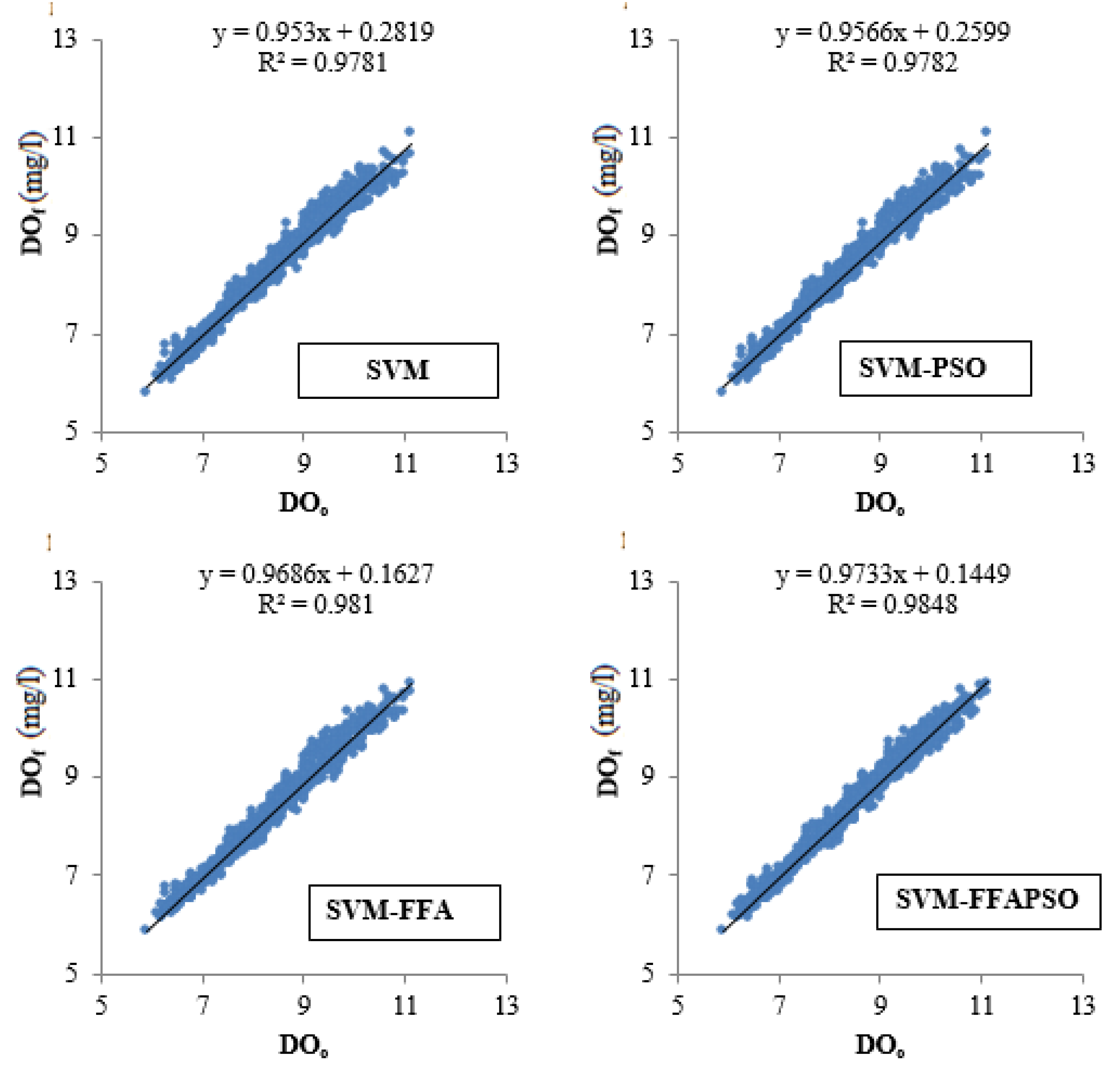
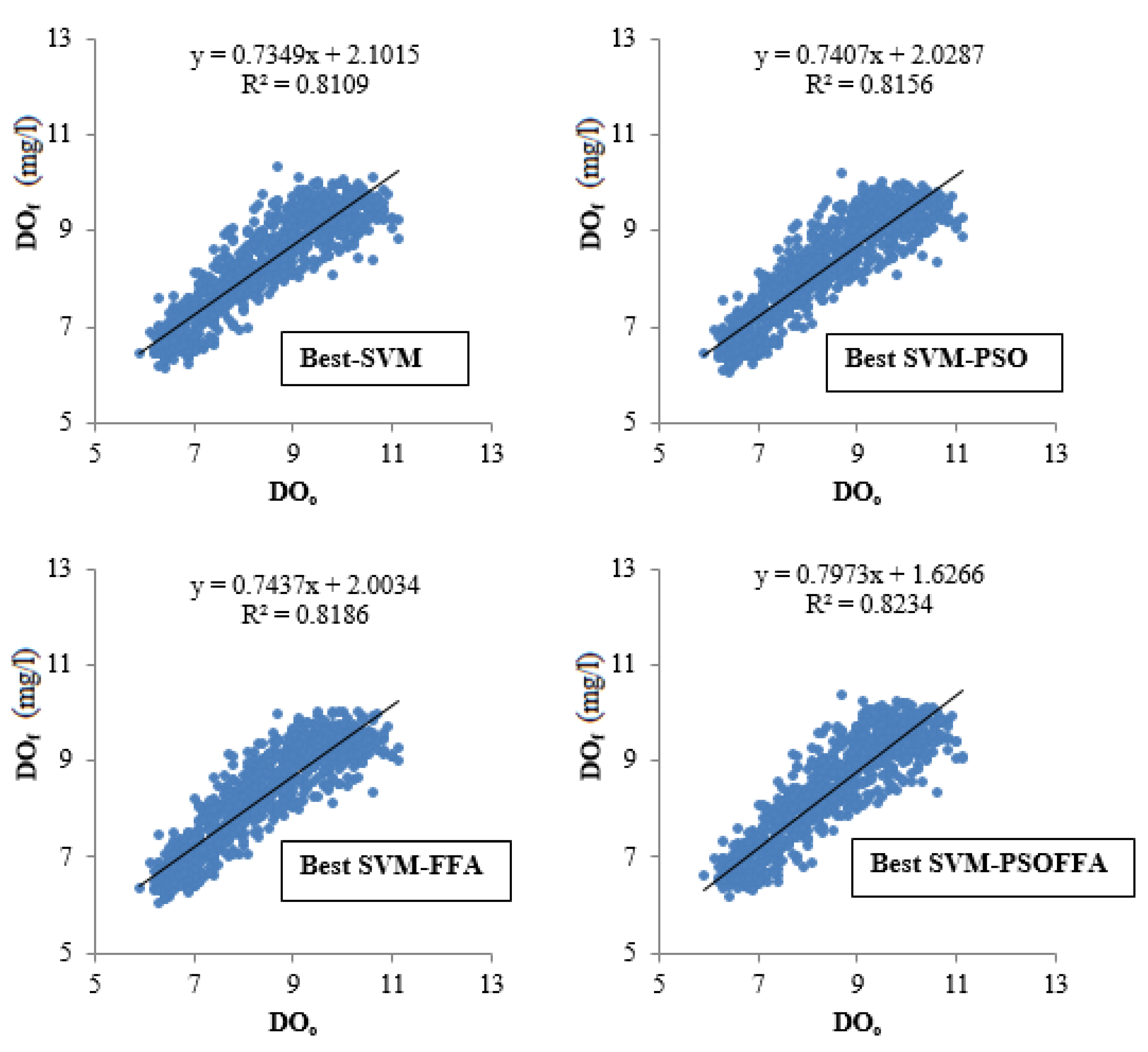
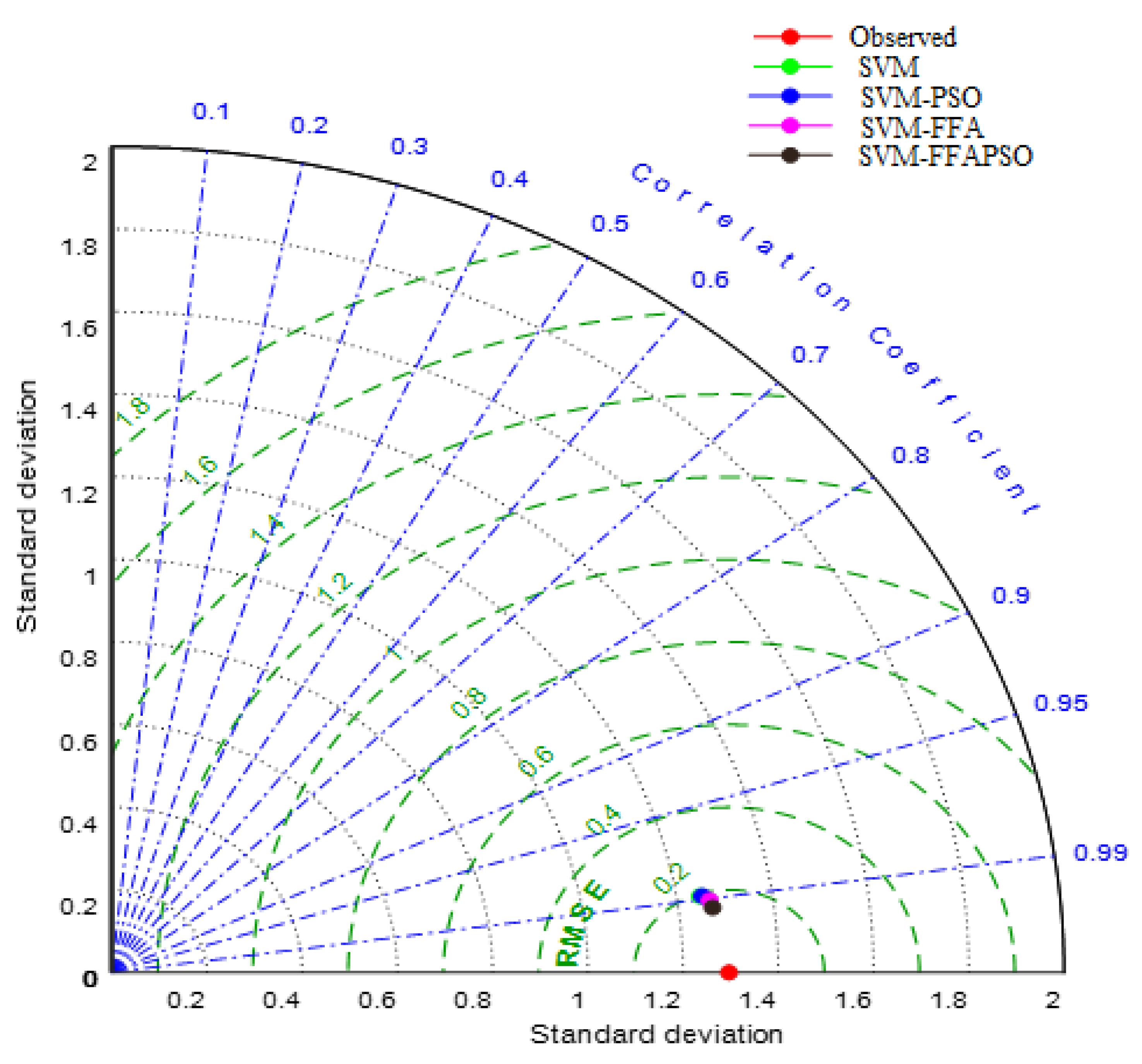
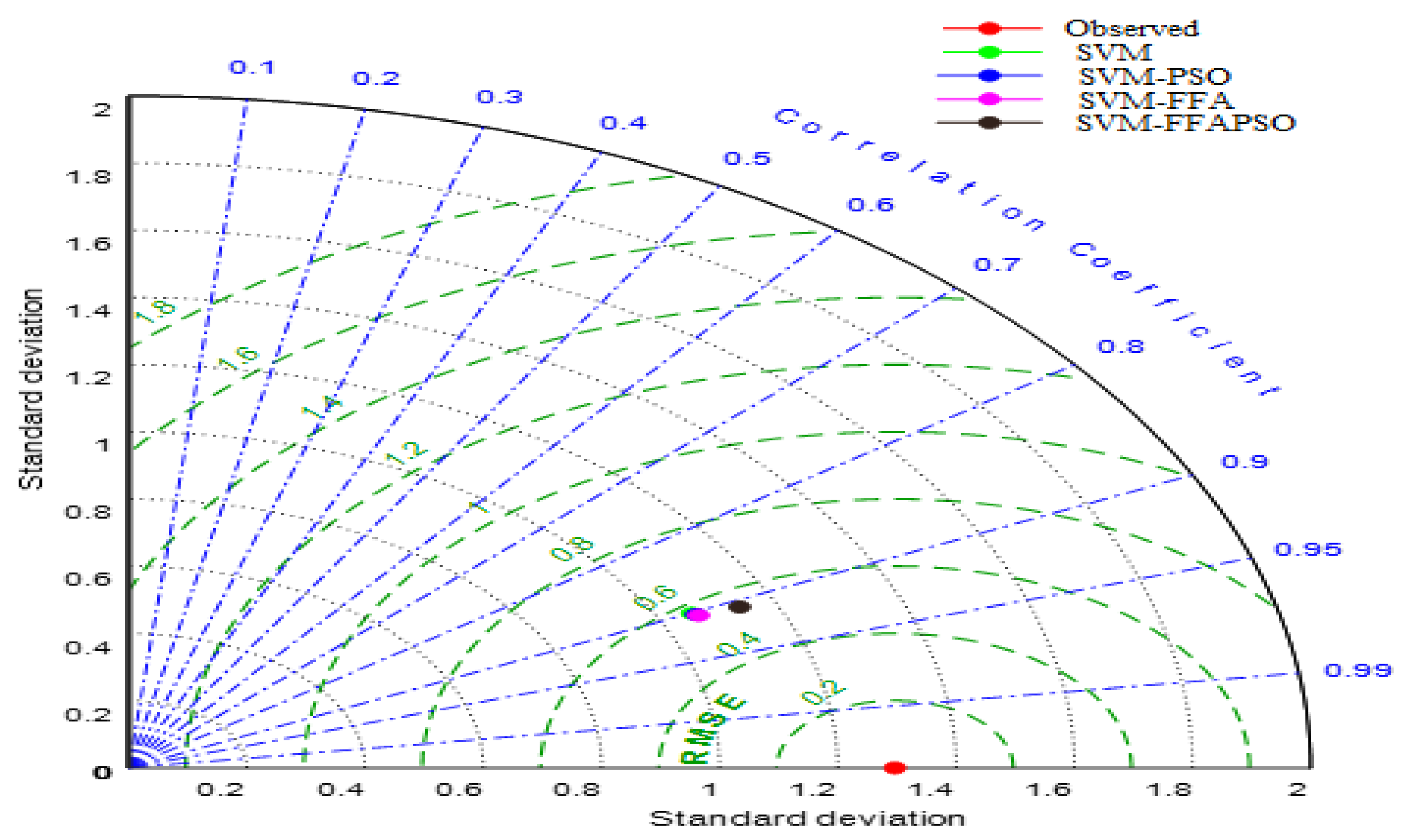
Figure 6 compares the testing outcomes of the optimal SVM–based models via scatter diagrams. It is evident from the fit line equations and R² values, the SVM–FFAPSO has less scattered estimates compared to other models and its performance is followed by the hybrid SVM–FFA and SVM–PSO. The Taylor diagram provided in Figure 7 tell us that the hybrid SVM–FFAPSO model has closer standard deviation to the observed DO concentration and it has the lowest RMSE and the highest correlation.

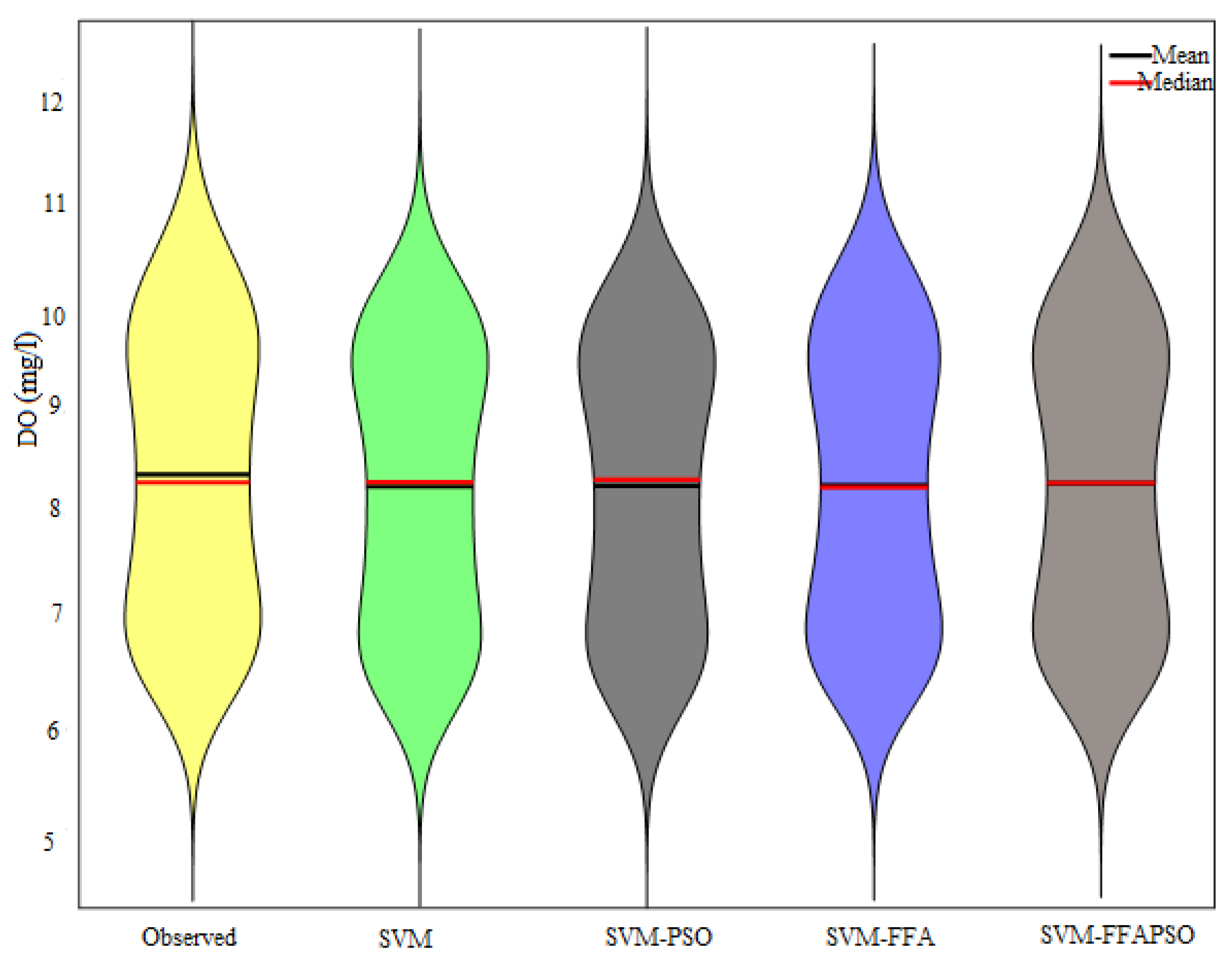
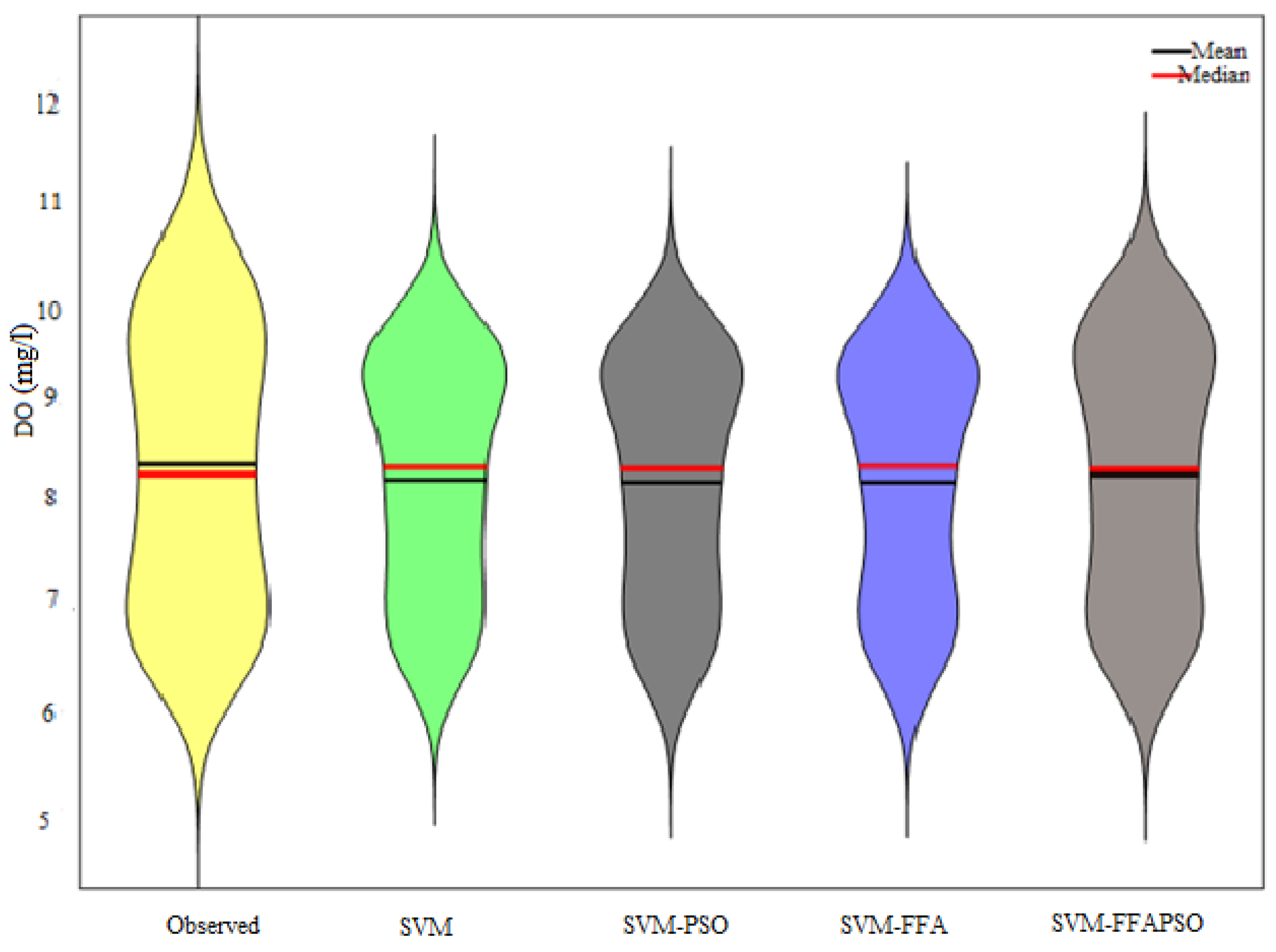
A Violin chart compares the distributions of the models’ estimation in Figure 8. It is seen from the figure that the proposed SVM–FFAPSO has closer distribution to the that of the observed DO values.

Figure 9 illustrates the scatterplot comparison of the SVM–based models’ outcomes in estimating 7-day ahead DO concentration. As seen from the fit line equations and determination coefficient values in the figure, the hybrid SVM–FFAPSO keeps its superiority in estimating t + 7 DO with slope coefficient and bias values closer to 1 and 0 and higher R² compared to other three models. Hybrid SVM–FFA and SVM–PSO also have better forecasting performance than the standard SVM model, as evident from the fit line equations closer to the ideal line equation (y = x) and higher R². It is clearly observed from the Taylor diagram given in Figure 10 that the hybrid SVM–FFAPSO model has superior accuracy over other models with respect to RMSE, correlation and standard deviation. The hybrid SVM–FFAPSO has closer standard deviation to the observed one and higher correlation and lower RSME compared to the SVM–FFA, SVM–PSO and standard SVM models. Figure 11 shows that the similarity between the distributions of the SVM–FFAPSO and observed values is higher compared to the other SVM–based models in estimating 7-day ahead DO concentration. It is clearly seen from the figure that the mean and median values of the hybrid SVM–FFAPSO are closer to the observed one and distribution of the estimates in the upper and lower parts (with respect to mean or medium) are more resembling the distributions of the target DO values. Comparison of Figure 5, Figure 6 and Figure 7 clearly indicates that increasing the time lag to 7 considerably decreased the models’ accuracy in estimating DO concentration.

Singh et al. [63] predicted the DO of the Gomti River, India using neural networks and they found correlation coefficient, R of 0.76 from the best model in the test stage. Ranković et al. [64] modeled the DO of the Gruza Reservoir, Serbia, considering the inputs of pH, temperature, nitrates, chloride and total phosphate. They obtained an R of 0.874 for the best model in the test stage. Heddam [65] used GRNN for modeling the DO of the Upper Klamath River, USA and they used T, pH, SC and SD as inputs. The correlation coefficient (R) of the best model (GRNN) was found to be 0.984 in the test stage. Elkiran et al. [66] investigated the accuracy of an ensemble method involving ANFIS, SVM and ARIMA in modeling DO of the Yamuna River, India using inputs BOD, COD, discharge, pH, Ammonia and water temperature. The best models produced a mean R of 0.969 from three stations considered in their study. In our study, the best SVM–FFAPSO model provided R of 0.992 in modeling DO of Fountain Creek, which indicates the good accuracy of the proposed model.

4. Conclusions

In this study, the viability of a new hybrid method, SVM–FFAPSO, was investigated for predicting DO concentration for multiple time steps. The outcomes of the model were compared with the standard SVM and hybrid SVM–FFA and SVM–PSO models. Various combinations of daily pH, T, EC and Q data acquired from Fountain Creek near Fountain, USA were used as inputs to the models to estimate 1-day to 7-day ahead DO. The implemented methods were assessed based on RMSE, MAE, NSE, R² and graphical inspections (scatterplots, Taylor and violin charts). Analysis outcomes showed that the SVM–FFAPSO outperformed the other methods in estimating DO in all time steps. Tuning SVM hyperparameters using FFA, PSO and FFAPSO improved the accuracy of the standard SVM method in forecasting multi-time step daily DO concentration. The proposed hybrid SVM–FFAPSO improved the estimation accuracy of the standard SVM with respect to the RMSE, MAE, NSE and R² by 13.9%, 22%, 0.52% and 1.83% in estimating 1-day ahead DO concentration in the test stage, respectively. The corresponding improvements were, respectively, obtained as 26.4%, 24.1%, 13.8% and 15.9% in estimating 7-day ahead DO concentration. The outcomes recommended the employment of hybrid SVM–FFAPSO in DO modeling.

References

1. Gupta, S.; Gupta, S.K. A critical review on water quality index tool: Genesis, evolution and future directions. Ecol. Inform. 2021, 63, 101299. [Google Scholar] [CrossRef]
2. Hmoud Al-Adhaileh, M.; Waselallah Alsaade, F. Modelling and Prediction of Water Quality by Using Artificial Intelligence. Sustainability 2021, 13, 4259. [Google Scholar] [CrossRef]
3. Yin, L.; Fu, L.; Wu, H.; Xia, Q.; Jiang, Y.; Tan, J.; Guo, Y. Modeling dissolved oxygen in a crab pond. Ecol. Model. 2021, 440, 109385. [Google Scholar] [CrossRef]
4. Alizamir, M.; Kisi, O.; Adnan, R.M.; Kuriqi, A. Modelling reference evapotranspiration by combining neuro-fuzzy and evolutionary strategies. Acta Geophys. 2020, 68, 1113–1126. [Google Scholar] [CrossRef]
5. Adnan, R.; Parmar, K.; Heddam, S.; Shahid, S.; Kisi, O. Suspended Sediment Modeling Using a Heuristic Regression Method Hybridized with Kmeans Clustering. Sustainability 2021, 13, 4648. [Google Scholar] [CrossRef]
6. Kisi, O.; Shiri, J.; Karimi, S.; Adnan, R.M. Three Different Adaptive Neuro Fuzzy Computing Techniques for Forecasting Long-Period Daily Streamflows. In Big Data in Engineering Applications; Springer: Singapore, 2018; pp. 303–321. [Google Scholar]
7. Adnan, R.M.; Mostafa, R.R.; Kisi, O.; Yaseen, Z.M.; Shahid, S.; Zounemat-Kermani, M. Improving streamflow prediction using a new hybrid ELM model combined with hybrid particle swarm optimization and grey wolf optimization. Knowl. Based Syst. 2021, 230, 107379. [Google Scholar] [CrossRef]
8. Yuan, X.; Chen, C.; Lei, X.; Yuan, Y.; Adnan, R.M. Monthly runoff forecasting based on LSTM–ALO model. Stoch. Environ. Res. Risk Assess. 2018, 32, 2199–2212. [Google Scholar] [CrossRef]
9. Tao, H.; Al-Sulttani, A.O.; Ameen, A.M.S.; Ali, Z.H.; Al-Ansari, N.; Salih, S.Q.; Mostafa, R.R. Training and Testing Data Division Influence on Hybrid Machine Learning Model Process: Application of River Flow Forecasting. Complexity 2020, 2020, 8844367. [Google Scholar] [CrossRef]
10. Adnan, R.M.; Mostafa, R.R.; Islam, A.R.M.T.; Gorgij, A.D.; Kuriqi, A.; Kisi, O. Improving Drought Modeling Using Hybrid Random Vector Functional Link Methods. Water 2021, 13, 3379. [Google Scholar] [CrossRef]
11. Sha, J.; Li, X.; Zhang, M.; Wang, Z.L. Comparison of Forecasting Models for Real-Time Monitoring of Water Quality Parameters Based on Hybrid Deep Learning Neural Networks. Water 2021, 13, 1547. [Google Scholar] [CrossRef]
12. Fijani, E.; Barzegar, R.; Deo, R.; Tziritis, E.; Skordas, K. Design and implementation of a hybrid model based on two-layer decomposition method coupled with extreme learning machines to support real-time environmental monitoring of water quality parameters. Sci. Total Environ. 2019, 648, 839–853. [Google Scholar] [CrossRef] [PubMed]
13. Chia, S.L.; Chia, M.Y.; Koo, C.H.; Huang, Y.F. Integration of advanced optimization algorithms into least-square support vector machine (LSSVM) for water quality index prediction. Water Supply 2021, 22, 951–1963. [Google Scholar] [CrossRef]
14. Heddam, S.; Kim, S.; Danandeh Mehr, A.; Zounemat-Kermani, M.; Malik, A.; Elbeltagi, A.; Kisi, O. Predicting dissolved oxygen concentration in river using new advanced machines learning: Long-short term memory (LSTM) deep learning. Comput. Earth Environ. Sci. 2021, 1, 1–20. [Google Scholar] [CrossRef]
15. Zhi, W.; Feng, D.; Tsai, W.P.; Sterle, G.; Harpold, A.; Shen, C.; Li, L. From hydrometeorology to river water quality: Can a deep learning model predict dissolved oxygen at the continental scale? Environ. Sci. Technol. 2021, 55, 2357–2368. [Google Scholar] [CrossRef] [PubMed]
16. Tasnim, B.; Jamily, J.A.; Fang, X.; Zhou, Y.; Hayworth, J.S. Simulating diurnal variations of water temperature and dissolved oxygen in shallow Minnesota lakes. Water 2021, 13, 1980. [Google Scholar] [CrossRef]
17. Dabrowski, J.J.; Rahman, A.; Pagendam, D.E.; George, A. Enforcing mean reversion in state space models for prawn pond water quality forecasting. Comput. Electron. Agric. 2020, 168, 105120. [Google Scholar] [CrossRef]
18. Cao, X.; Liu, Y.; Wang, J.; Liu, C.; Duan, Q. Prediction of dissolved oxygen in pond culture water based on K-means clustering and gated recurrent unit neural network. Aquac. Eng. 2020, 91, 102122. [Google Scholar] [CrossRef]
19. Zhao, N.; Fan, Z.; Zhao, M. A New Approach for Estimating Dissolved Oxygen Based on a High-Accuracy Surface Modeling Method. Sensors 2021, 21, 3954. [Google Scholar] [CrossRef] [PubMed]
20. Salih, S.Q.; Alakili, I.; Beyaztas, U.; Shahid, S.; Yaseen, Z.M. Prediction of dissolved oxygen, biochemical oxygen demand, and chemical oxygen demand using hydrometeorological variables: Case study of Selangor River, Malaysia. Environ. Dev. Sustain. 2021, 23, 8027–8046. [Google Scholar] [CrossRef]
21. Heddam, S. New modelling strategy based on radial basis function neural network (RBFNN) for predicting dissolved oxygen concentration using the components of the Gregorian calendar as inputs: Case study of Clackamas River, Oregon, USA. Model. Earth Syst. Environ. 2016, 2, 1–5. [Google Scholar] [CrossRef] [Green Version]
22. Rozario, A.P.; Devarajan, N. Monitoring the quality of water in shrimp ponds and forecasting of dissolved oxygen using Fuzzy C means clustering based radial basis function neural networks. J. Ambient Intell. Humaniz. Comput. 2021, 12, 4855–4862. [Google Scholar] [CrossRef]
23. Keshtegar, B.; Heddam, S.; Hosseinabadi, H. The employment of polynomial chaos expansion approach for modeling dissolved oxygen concentration in river. Environ. Earth Sci. 2019, 78, 34. [Google Scholar] [CrossRef]
24. Tiyasha, T.; Tung, T.M.; Bhagat, S.K.; Tan, M.L.; Jawad, A.H.; Mohtar, W.H.M.W.; Yaseen, Z.M. Functionalization of remote sensing and on-site data for simulating surface water dissolved oxygen: Development of hybrid tree-based artificial intelligence models. Mar. Pollut. Bull. 2021, 170, 112639. [Google Scholar] [CrossRef] [PubMed]
25. Heddam, S. Intelligent Data Analytics Approaches for Predicting Dissolved Oxygen Concentration in River: Extremely Randomized Tree versus Random Forest, MLPNN and MLR. In Intelligent Data Analytics for Decision-Support Systems in Hazard Mitigation; Springer: Singapore, 2021; pp. 89–107. [Google Scholar] [CrossRef]
26. Nacar, S.; Mete, B.; Bayram, A. Estimation of daily dissolved oxygen concentration for river water quality using conventional regression analysis, multivariate adaptive regression splines, and TreeNet techniques. Environ. Monit. Assess. 2020, 192, 752. [Google Scholar] [CrossRef] [PubMed]
27. Yang, F.; Moayedi, H.; Mosavi, A. Predicting the Degree of Dissolved Oxygen Using Three Types of Multi-Layer Perceptron-Based Artificial Neural Networks. Sustainability 2021, 13, 9898. [Google Scholar] [CrossRef]
28. Zhu, C.; Liu, X.; Ding, W. Prediction model of dissolved oxygen based on FOA-LSSVR. In Proceedings of the 2017 36th Chinese Control Conference (CCC), Dalian, China, 26–28 July 2017; pp. 9819–9823. [Google Scholar] [CrossRef]
29. Raheli, B.; Aalami, M.T.; El-Shafie, A.; Ghorbani, M.A.; Deo, R.C. Uncertainty assessment of the multilayer perceptron (MLP) neural network model with implementation of the novel hybrid MLP-FFA method for prediction of biochemical oxygen demand and dissolved oxygen: A case study of Langat River. Environ. Earth Sci. 2017, 76, 503. [Google Scholar] [CrossRef]
30. Deng, C.; Wei, X.; Guo, L. Application of neural network based on PSO algorithm in prediction model for dissolved oxygen in fishpond. In Proceedings of the 2006 6th World Congress on Intelligent Control and Automation, Guilin, China, 21–23 June 2006; Volume 2, pp. 9401–9405. [Google Scholar] [CrossRef]
31. Song, C.; Yao, L.; Hua, C.; Ni, Q. A novel hybrid model for water quality prediction based on synchrosqueezed wavelet transform technique and improved long short-term memory. J. Hydrol. 2021, 603, 126879. [Google Scholar] [CrossRef]
32. Zhang, K.; Wu, L. Using a fractional order grey seasonal model to predict the dissolved oxygen and pH in the Huaihe River. Water Sci. Technol. 2021, 83, 475–486. [Google Scholar] [CrossRef]
33. Cao, S.; Zhou, L.; Zhang, Z. Prediction of Dissolved Oxygen Content in Aquaculture Based on Clustering and Improved ELM. IEEE Access 2021, 9, 40372–40387. [Google Scholar] [CrossRef]
34. Dehghani, R.; Torabi Poudeh, H.; Izadi, Z. Dissolved oxygen concentration predictions for running waters with using hybrid machine learning techniques. Modeling Earth Syst. Environ. 2021, 6, 1–15. [Google Scholar] [CrossRef]
35. Miao, X.; Deng, C.; Li, X.; Gao, Y.; He, D. A hybrid neural network and genetic algorithm model for predicting dissolved oxygen in an aquaculture pond. In Proceedings of the 2010 International Conference on Web Information Systems and Mining, Sanya, China, 23–24 October 2010; Volume 1, pp. 415–419. [Google Scholar] [CrossRef]
36. Shah, M.I.; Javed, M.F.; Alqahtani, A.; Aldrees, A. Environmental assessment based surface water quality prediction using hyper-parameter optimized machine learning models based on consistent big data. Process Saf. Environ. Prot. 2021, 151, 324–340. [Google Scholar] [CrossRef]
37. Zhou, X.; Li, D.; Zhang, L.; Duan, Q. Application of an adaptive PID controller enhanced by a differential evolution algorithm for precise control of dissolved oxygen in recirculating aquaculture systems. Biosyst. Eng. 2021, 208, 186–198. [Google Scholar] [CrossRef]
38. Jiang, J.; Tang, S.; Liu, R.; Sivakumar, B.; Wu, X.; Pang, T. A hybrid wavelet-Lyapunov exponent model for river water quality forecast. J. Hydroinform. 2021, 23, 864–878. [Google Scholar] [CrossRef]
39. Huang, J.; Huang, Y.; Hassan, S.G.; Xu, L.; Liu, S. Dissolved oxygen content interval prediction based on auto regression recurrent neural network. J. Ambient. Intell. Humaniz. Comput. 2021, 12, 1–10. [Google Scholar] [CrossRef]
40. Li, W.; Wei, Y.; An, D.; Jiao, Y.; Wei, Q. LSTM-TCN: Dissolved oxygen prediction in aquaculture, based on combined model of long short-term memory network and temporal convolutional network. Environ. Sci. Pollut. Res. 2022, 29, 1–12. [Google Scholar] [CrossRef] [PubMed]
41. Yang, H.; Liu, S. A prediction model of aquaculture water quality based on multiscale decomposition. Math. Biosci. Eng. 2021, 18, 7561–7579. [Google Scholar] [CrossRef] [PubMed]
42. Moghadam, S.V.; Sharafati, A.; Feizi, H.; Marjaie, S.M.S.; Asadollah, S.B.H.S.; Motta, D. An efficient strategy for predicting river dissolved oxygen concentration: Application of deep recurrent neural network model. Environ. Monit. Assess 2021, 193, 798. [Google Scholar] [CrossRef] [PubMed]
43. Song, C.; Yao, L. Application of artificial intelligence based on synchrosqueezed wavelet transform and improved deep extreme learning machine in water quality prediction. Environ. Sci. Pollut. Res. 2022, 17, 1–17. [Google Scholar] [CrossRef] [PubMed]
44. Wu, Y.; Sun, L.; Sun, X.; Wang, B. A hybrid XGBoost-ISSA-LSTM model for accurate short-term and long-term dissolved oxygen prediction in ponds. Environ. Sci. Pollut. Res. 2021, 29, 18142–18159. [Google Scholar] [CrossRef] [PubMed]
45. Cortes, C.; Vapnik, V. Support-vector networks. Mach. Learn. 1995, 20, 273–297. [Google Scholar] [CrossRef]
46. Kisi, O.; Parmar, K.S. Application of least square support vector machine and multivariate adaptive regression spline models in long term prediction of river water pollution. J. Hydrol. 2016, 534, 104–112. [Google Scholar] [CrossRef]
47. Kisi, O.; Parmar, K.S.; Soni, K.; Demir, V. Modeling of air pollutants using least square support vector regression, multivariate adaptive regression spline, and M5 model tree models. Air Qual. Atmos. Heal. 2017, 10, 873–883. [Google Scholar] [CrossRef]
48. Singh, S.; Parmar, K.S.; Makkhan, S.J.S.; Kaur, J.; Peshoria, S.; Kumar, J. Study of ARIMA and least square support vector machine (LS-SVM) models for the prediction of SARS-CoV-2 confirmed cases in the most affected countries. Chaos Solitons Fractals 2020, 139, 110086. [Google Scholar] [CrossRef] [PubMed]
49. Suykens, J.A.K.; Vandewalle, J. Least squares support vector machine classifiers. Neural. Process. Lett. 1999, 9, 293–300. [Google Scholar] [CrossRef]
50. Yang, X.S. Firefly algorithm, stochastic test functions and design optimization. Int. J. Bio-Inspired Comput. 2010, 2, 78–84. [Google Scholar] [CrossRef]
51. Gandomi, A.H.; Yang, X.S.; Alavi, A.H. Mixed variable structural optimization using Firefly Algorithm. Comput. Struct. 2011, 89, 2325–2336. [Google Scholar] [CrossRef]
52. Poursalehi, N.; Zolfaghari, A.; Minuchehr, A.; Moghaddam, H.K. Continuous firefly algorithm applied to PWR core pattern enhancement. Nucl. Eng. Des. 2013, 258, 107–115. [Google Scholar] [CrossRef]
53. Kennedy, J.; Eberhart, R.C. Particle swarm optimization. In Proceedings of the IEEE International Conference on Neural Networks, (Perth, Australia); IEEE Service Center: Piscataway, NJ, USA, 1995; pp. 1942–1948. [Google Scholar]
54. Eberhart, R.C.; Kennedy, J. A new optimizer using particle swarm theory. In Proceedings of the Sixth International Symposium on Micro Machine and Human Science (Nagoya, Japan); IEEE Service Center: Piscataway, NJ, USA, 1995; pp. 39–43. [Google Scholar]
55. Poli, R.; Kennedy, J.; Blackwell, T. Particle swarm optimization. Swarm Intell. 2007, 1, 33–57. [Google Scholar] [CrossRef]
56. Wang, D.; Tan, D.; Liu, L. Particle swarm optimization algorithm: An overview. Soft Comput. 2018, 22, 387–408. [Google Scholar] [CrossRef]
57. Aydilek, I.B. A hybrid firefly and particle swarm optimization algorithm for computationally expensive numerical problems. Appl. Soft Comp. 2018, 66, 232–249. [Google Scholar] [CrossRef]
58. Adnan, R.M.; Jaafari, A.; Mohanavelu, A.; Kisi, O.; Elbeltagi, A. Novel Ensemble Forecasting of Streamflow Using Locally Weighted Learning Algorithm. Sustainability 2021, 13, 5877. [Google Scholar] [CrossRef]
59. Adnan, R.M.; Liang, Z.; El-Shafie, A.; Zounemat-Kermani, M.; Kisi, O. Prediction of Suspended Sediment Load Using Data-Driven Models. Water 2019, 11, 2060. [Google Scholar] [CrossRef] [Green Version]
60. Banadkooki, F.B.; Singh, V.P.; Ehteram, M. Multi-timescale drought prediction using new hybrid artificial neural network models. Nat. Hazards 2021, 106, 2461–2478. [Google Scholar] [CrossRef]
61. Başakın, E.E.; Ekmekcioğlu, Ö.; Özger, M. Drought prediction using hybrid soft-computing methods for semi-arid region. Model. Earth Syst. Environ. 2021, 7, 2363–2371. [Google Scholar] [CrossRef]
62. Adnan, R.M.; Petroselli, A.; Heddam, S.; Santos, C.A.G.; Kisi, O. Short term rainfall-runoff modelling using several machine learning methods and a conceptual event-based model. Stoch. Environ. Res. Risk Assess. 2021, 35, 597–616. [Google Scholar] [CrossRef]
63. Singh, K.P.; Basant, A.; Malik, A.; Jain, G. Artificial neural network modeling of the river water quality—A case study. Ecol. Model. 2009, 220, 888–895. [Google Scholar] [CrossRef]
64. Ranković, V.; Radulović, J.; Radojević, I.; Ostojić, A.; Čomić, L. Neural network modeling of dissolved oxygen in the Gruža reservoir, Serbia. Ecol. Model. 2010, 221, 1239–1244. [Google Scholar] [CrossRef]
65. Heddam, S. Generalized regression neural network-based approach for modelling hourly dissolved oxygen concentration in the Upper Klamath River, Oregon, USA. Environ. Technol. 2014, 35, 1650–1657. [Google Scholar] [CrossRef] [PubMed]
66. Elkiran, G.; Nourani, V.; Abba, S.I. Multi-step ahead modeling of river water quality parameters using ensemble artificial intelligence-based approach. J. Hydrol. 2019, 577, 123962. [Google Scholar] [CrossRef]
Figure 1. Location of study site.
Sustainability 14 03470 g001
Figure 2. Structure of SVM model.
Sustainability 14 03470 g002
Figure 3. Basic Working Flow of SVM–FFA Model.
Sustainability 14 03470 g003
Figure 4. Basic Working Flow of SVM–PSO Model.
Sustainability 14 03470 g004
Figure 5. Basic Working Flow of SVM–FFAPSO Model.
Sustainability 14 03470 g005
Figure 6. Scatterplots of the observed and estimated daily DO concentrations by different SVM based models in the test period using best input combination.
Sustainability 14 03470 g006
Figure 7. Taylor diagram of daily DO concentrations by different SVM based models in the test period using best input combination.
Sustainability 14 03470 g007
Figure 8. Violin charts of daily DO concentrations by different SVM based models in the test period using best input combination.
Sustainability 14 03470 g008
Figure 9. Scatterplots of the observed and estimated multistep (7 days ahead) DO concentrations by different SVM based models in the test period using best input combination.
Sustainability 14 03470 g009
Figure 10. Taylor diagram of multistep (7 days ahead) DO concentrations by different SVM based models in the test period using best input combination.
Sustainability 14 03470 g010
Figure 11. Violin charts of multistep (7 days ahead) DO concentrations by different SVM based models in the test period using best input combination.
Sustainability 14 03470 g011