
Collaborative Optimization of Vehicle and Crew Scheduling for a Mixed Fleet with Electric and Conventional Buses


1
College of Engineering, Shenyang Agricultural University, Shenyang 110866, China
2
Department of Transport & Planning, Delft University of Technology, 2600 AA Delft, The Netherlands
3
College of Forensic Sciences, Criminal Investigation Police University of China, Shenyang 110854, China
*
Author to whom correspondence should be addressed.
Sustainability 2022, 14(6), 3627; https://0-doi-org.brum.beds.ac.uk/10.3390/su14063627
Submission received: 13 February 2022
/
Revised: 17 March 2022
/
Accepted: 17 March 2022
/
Published: 19 March 2022
(This article belongs to the Special Issue Sustainable Transportation Electrification: Policy, Planning and Operation)
Abstract
:Replacing conventional buses with electric buses is in line with the concept of sustainable development. However, electric buses have the disadvantages of short driving range and high purchase price. Many cities must implement a semi-electrification strategy for bus routes. In this paper, a bi-level, multi-objective programming model is established for the collaborative scheduling problem of vehicles and drivers on a bus route served by the mixed bus fleet. The upper-layer model minimizes the operation cost and economic cost of carbon emission to optimize the vehicle and charging scheme; while the lower-layer model tries to optimize the crew-scheduling scheme with the objective of minimizing driver wages and maximizing the degree of bus-driver specificity, considering the impact of drivers’ labor restrictions. Then, the improved multi-objective particle swarm algorithm based on an -constraint processing mechanism is used to solve the problem. Finally, an actual bus route is taken as an example to verify the effectiveness of the model. The results show that the established model can reduce the impact of unbalanced vehicle scheduling in mixed fleets on crew scheduling, ensure the degree of driver–bus specificity to standardize operation, and save the operation cost and driver wage.
1. Introduction
1.1. Background
To tackle climate change and curb carbon emissions, many countries worldwide have pledged to partially or completely replace their conventional buses with electric ones in the coming decades [1,2]. Electric buses (EBs) are clean, non-polluting, and energy-efficient. They are consistent with the concept of sustainable transportation and are conducive to cost savings for a long time. However, their purchase price is high, between USD 300,000 and USD 900,000 per vehicle [3], which is about 2–3 times the price of conventional buses (CBs), and the upfront purchase cost brings great pressure. Thus, many cities have had to delay the electrification of buses or reduce the proportion of EBs in their fleets. During this period, EBs and CBs need to jointly serve one bus route.
EBs consume less electricity per unit mileage, which is helpful for reducing the operation cost of bus routes, but their driving range is limited and their charging time is long [4]. In contrast, the cruising range of CBs is long, and the refueling time is very short, but the fuel consumption per unit mileage is large, which leads to increases in bus route operation costs and carbon emissions. For a mixed fleet with a fixed electrification ratio, it is usually necessary to comprehensively consider operation costs and carbon emissions for vehicle scheduling. Here, CBs are the supplement of EBs, and they have been allocated to shorter trips in priority or smaller numbers of trips [5].
This uneven vehicle-scheduling scheme will exacerbate the crew-scheduling problem, which makes the one-driver-one-bus service mode no longer applicable. Compared with the non–one-driver-one-bus mode, the driver is more familiar with the bus conditions in the one-driver-one-bus situation, and it is also convenient for bus companies to manage vehicles and drivers. In addition, since the buses’ travel time is greatly affected by road traffic conditions, passenger boarding and alighting, and the number of signalized intersections with a high amount of randomness, the one-driver-one-bus service mode can more flexibly deal with the problem of bus delays at the departure or destination station. Therefore, considering the specificity of the bus driver, in which the same driver serves the same bus as much as possible, collaboratively optimizing vehicle and crew scheduling for a mixed fleet of EBs and CBs could not only help reduce the operation costs of bus companies but also help standardize operations and improve bus service quality.
1.2. Literature Review
In view of the scheduling problems for vehicles and crews using a mixed fleet with electric and conventional buses, existing studies can be roughly divided into two groups in terms of optimization structures, namely the two-phase sequence method and the collaborative scheduling method.
- 1.
- Two-phase sequence method
In the two-phase sequence method, the vehicle-scheduling scheme for the mixed fleet is first determined considering the travel time feasibility and the service integrity of EBs, and then the crew-scheduling scheme is optimized considering labor regulations [6]. The input of the crew-scheduling model depends on the output of the vehicle-scheduling model, and it can reduce the complexity of the combinatorial optimization problem.
For the vehicle-scheduling problem, most studies are only focused on the conventional bus [7,8,9,10] or pure electric bus [11,12,13,14]. Only a few studies focus on the vehicle-scheduling problem of mixed fleets of CBs and pure EBs. Zhou et al. (2020) proposed a multi-objective bi-level programming model to optimize the vehicle and charging scheduling of a mixed bus fleet [15]. Under range and refueling constraints, Li et al. (2019) developed an integer linear programming model for multiple-depot vehicle-scheduling problems with multiple vehicle types, including EBs. Additionally, they developed a simplified formulation to handle larger-scale problems for approximate solutions, based on the time-space flow network [16]. Ayman et al. (2022) presented a novel framework for the data-driven prediction of trip-level energy use for mixed-vehicle transit fleets and the optimization of vehicle assignments [17]. Lu et al. (2021) proposed a joint optimal scheduling model for a mixed bus fleet under micro driving conditions, and it was validated based on data from Beijing [18]. Rinaldi et al. (2020) developed a mixed-integer linear program model to address the problem of vehicle scheduling with a mixed fleet of electric and hybrid/non-electric buses and used an ad hoc decomposition scheme to enhance the scalability of the proposed model [4]. Duan et al. (2021) proposed an optimal framework for reforming the mixed operation schedule for electric buses and traditional fuel buses under stochastic trip times [19].
Regarding the crew-scheduling problem, Smith and Wren (1988) described a bus crew-scheduling system based on a set covering formulation and used many heuristics to keep it to a manageable size [20]. Chen and Niu (2012) presented an approach for solving the bus crew-scheduling problem, which considers early, day, and late duty modes with time-shift and work-intensity constraints [21]. Ma et al. (2016) investigated a variable neighborhood search algorithm for solving real-world bus–driver scheduling problems [22]. Ma et al. (2017) proposed a model considering fairness in the bus crew-scheduling problem and used a hybrid ant colony optimization algorithm to solve it [23]. Kang et al. (2019) developed an integer linear programming model to deal with the bus- and driver-scheduling problems with mealtime windows for a single public transport bus route [24]. Lin et al. (2020) proposed an integrated scheduling and rostering model for bus drivers and devised a branch-and-price-and-cut algorithm to solve the complex problem [25]. Rahman et al. (2020) presented an approach for rescheduling the bus crew’s timetable in the event of late for relief and took the multi-agent system to adapt dynamic environments [26]. Perumal et al. (2021) proposed a column generation approach that attempted to minimize operational expense for the driver scheduling problem with staff cars [27].
- 2.
- Collaborative scheduling method
The above-mentioned interaction between the vehicle-scheduling problem and the crew-scheduling problem is considered for cooperatively finding the optimal vehicle and crew-scheduling scheme, which may be a result of balance or compromise. In recent years, more and more scholars have begun to pay attention to the research on integrated vehicle- and crew-scheduling problems. Boyer et al. (2018) proposed a mixed-integer linear programming model and a variable neighborhood search for the flexible vehicle- and crew-scheduling problem [28]. Amberg et al. (2019) examined combined vehicle- and crew-scheduling in public bus transit in the context of both robust and cost-efficient resource allocation [29]. Simoes et al. (2021) proposed a matheuristic algorithm for solving the multiple-depot vehicle and crew-scheduling problem [30]. Andrade-Michel et al. (2021) proposed the bus-vehicle- and reliable-driver-scheduling problem considering drivers’ reliability information to reduce the number of non-covered trips throughout the day and thus improve the user’s satisfaction [31]. Perumal et al. (2021) introduced an integrated electric vehicle- and crew-scheduling problem with given a set of timetabled trips and recharging stations [32].
Under the framework of the two-phase sequence method, the output of the crew-scheduling scheme depends on the input of the vehicle-scheduling scheme, and it is difficult to achieve the optimal total system cost. Unlike the optimization problem of the vehicle and crew scheduling for a single bus type, CBs have become supplements of EBs in the mixed bus fleet, and the operating intensity varies greatly between different bus types, due to the respective characteristics of EBs and CBs. In this case, to ensure the rationality and fairness of the driver’s working time, the driver may need to drive multiple buses, which brings inconvenience to the convenience of operation and management of bus companies and the reliability of bus services.
1.3. Contributions
The purpose of this paper is to collaboratively optimize the vehicle-scheduling scheme and crew-scheduling scheme of the mixed fleet, considering the operation costs, carbon emissions, driver wages, and the degree of driver–bus specificity. The main contributions of this paper are as follows: (i) Considering the feasibility of travel time and the integrity of service trips, a vehicle-scheduling optimization model for a mixed fleet of EBs and CBs is established to minimize the operation costs and carbon emissions. (ii) A quantification method of driver–bus specificity is proposed, and a crew-scheduling optimization model is established under the constraints of labor regulations, with the objective of minimizing driver wages and maximizing driver–bus specificity. (iii) For the collaborative scheduling problem of vehicles and drivers in mixed bus fleets, we design a bi-level multi-objective programming model, which is solved by an improved multi-objective particle swarm algorithm based on the -constraint processing mechanism.
2. Methodology
2.1. Notation Definition
Let the set of EBs be , the set of CBs be , and the set of drivers be . A service trip refers to a round-trip operation of the bus between the departure and terminal stations of the route. A driving trip is defined as a driver driving a designated bus from the departure station to the terminal station and then returning to the departure station. The I service trips within the daily operating time are labeled in turn according to the timetable, and service trips i and j are two adjacent trips that a certain bus needs to run. The numbers of each driving trip correspond to those of service trips. EBs use their idle time to recharge during the day. The time from the beginning of charging to the end of charging constitutes a charging trip, and the set of charging trips is recorded as . The route has a single depot for electric buses to charge, and for drivers to rest during shift changes, assuming that the number of charging facilities in it is adequate.
We define a binary variable if service trips i and j are adjacent trips run by EB k, ; otherwise . We define a binary variable if service trips i and j are adjacent trips run by CB h, ; otherwise, . The variable represents whether the driver g drives EB k to complete the service trip i. Variable represents whether the driver g drives CB h to complete the service trip i. Let indicate that EB k is charged during charging trip r; otherwise, .
Aiming at the collaborative scheduling problem of vehicles and crew in mixed bus fleets, we designed a bi-level multi-objective programming model, as shown in Figure 1. The upper layer is the vehicle-scheduling model for a bus fleet mixed with EBs and CBs that minimize the operation cost and carbon emissions [15,16]. The lower layer is the crew-scheduling model that minimizes the wages of drivers [21,27] and maximizes the degree of driver–bus specificity. The degree of driver–bus specificity of the entire fleet is quantified by the variance of the number of possible vehicle swaps of drivers. In the upper-layer model, the connecting time between trips should be considered when arranging service trips for electric buses and traditional buses, and the time-of-use (TOU) power price policy and the energy consumption demand of subsequent service trips should be taken into account when arranging charging trips for electric buses. In the lower-layer model, the driver’s working hours should comply with labor regulations. Appendix A introduces the meaning of the main notation used in the mathematical model.
2.2. Vehicle Scheduling (Upper Layer)
The purpose of the vehicle-scheduling problem for a mixed bus fleet is to allocate suitable service trips for EBs together with CBs, while arranging charging trips for EBs. The vehicle-scheduling problem for a bus fleet mixed with EBs and CBs is the same as the CB scheduling problem in terms of optimization objectives, and it is expected to minimize operation costs and carbon emissions; in terms of constraints, both EBs and CBs need to consider the travel time feasibility, and EBs also need to consider the TOU power price policy and the integrity of the service trip (i.e., whether the remaining battery power of the bus at the start of the service trip can meet the needs of subsequent service trips).
2.2.1. Objective Functions
The operation cost of a mixed fleet includes the cost of electricity consumption for EBs and fuel consumption for CBs. The carbon emissions mainly come from CBs, as EBs can be regarded as having zero emissions. The optimization objective Z of the vehicle-scheduling problem can be expressed as:
where OCB is the operation cost of CBs, RMB; OEB is the operation cost of EBs, RMB; MCB is the carbon emission of the mixed fleet, g; is the economic coefficient of the carbon emission of the mixed fleet, RMB/g.
The operation cost of CBs is equal to the cumulative driving mileage during the daily operating time multiplied by the corresponding mileage cost per unit, as shown in Equation (2).
where, is the fuel cost per unit mileage of CB, RMB/km; is the trip length, km; indicates whether CB h starts the operation task of the day from the service trip j; indicates whether CB h ends the operation task of the day from the service trip i; is the distance between the depot and the departure station of the service trip j, km; is the distance between the depot and the departure station of the service trip i, km.
Unlike CBs, EBs need to recharge during the day. The unit electricity price of charging is affected by the TOU power price policy and differs between various time periods. Let be the set of time periods during daytime operating hours [33]. The operation cost of EBs is equal to the daytime charging cost plus the nighttime charging cost, as shown in Equation (3).
where is the unit electricity price of charging in the period q, RMB/kWh; is the charging time of EB k in the period q, h; is the charging power of EB, kW; is the unit electricity price of charging at night, RMB /kWh; is the rated battery capacity of EB k, kWh; is the remaining battery power of EB k when the daytime operation task is completed and the night charging plan has not yet started, kWh; is the upper limit of the battery state of charge (SOC) set to prevent overcharge damage to the battery, %.
The total carbon emission of CBs is equal to the product of the accumulated driving mileage during the daily operation and the average carbon emission per kilometer , as shown in Equation (4).
2.2.2. Constraints
In the process of vehicle scheduling, we need to ensure that the adjacent service trips run by the same EBs or CBs are time feasible, namely that any EB k or CB h has sufficient time to take service trip j after trip i. For CBs, it is only necessary to ensure that the difference between the departure time of service trip j and service trip i is greater than or equal to the travel time of service trip i, as shown in Equation (5). The travel time includes the running time on the route, the docking time at the stations, and the dwell time at the departure station. For EBs, it is also necessary to ensure that the addition of charging trips will not affect the punctuality of buses, as shown in Equation (6). Equation (7) is the constraint of charging time of EB k.
where and Thj are departure times specified in the timetables for service trips i and j run by CB h; is the travel time of CB h on service trip i, h; and are departure times specified in the timetables for service trips i and j run by EB k; is the travel time of EB k on the service trip i, h; is the charging time of EB k on charging trip r, h; is the minimum charging time of EB k, h; and is the remaining battery power when EB k ends the service trip i, kWh.
The remaining battery power at the end of any adjacent service trips i and j run by EB k satisfies:
where is the remaining battery power when EB k ends the service trip j, kWh, and is the energy consumption of EB k on the service trip j, kWh.
In addition to time feasibility, EBs also need to keep the integrity of service trips. If EB k does not charge after the service trip i and continues to run service trip j, it should be ensured that the remaining battery power of the bus at the end of the service trip i can meet the energy consumption demand of the service trip j. If EB k needs to charge after the service trip i, there should be enough battery power to return to the depot.
where and is the energy consumption of the EB k returning from the departure station of the service trip i to the depot, kWh, and is the lower limit of battery SOC set to prevent over-discharge damage to the battery, %.
In addition, in order to ensure the normal operation of bus routes, it is stipulated that each service trip can only be assigned to one EB or CB, and each service trip needs to be run.
2.3. Crew Scheduling (Lower Layer)
For a bus fleet where EBs and CBs are mixed, the daily service time of each bus varies greatly, and it is difficult for drivers to continuously drive the same bus. This has a great impact on the convenience of operation and management of public transit companies and the reliability of public transport services. The crew-scheduling problem addressed in this section is to comprehensively consider labor regulations and reasonably arrange drivers to complete the driving trips for minimizing driver wages and maximizing driver–bus specificity.
2.3.1. Objective Functions
Driver wages are determined by the hours a driver works daily, including base wage and overtime pay. Effective working hours refer to the driving time of the driver, which only includes the running time on the route and does not include the time when the vehicle stops at the stations. On-duty time refers to the time duration from the start of the driver’s check-in at work to the time of check-out after getting off work. The driver’s base wage is calculated cumulatively based on the effective labor cost of a single driving trip. When the driver’s on-duty time is longer than the specified working time, the overtime pay needs to be calculated additionally. Then, one of the optimization objective functions of the lower layer optimization model, the calculation method of the driver’s one-day wage, is shown in Equation (11).
where and are the effective working hours, respectively, of CB h and EB k on driving trip i, h; and are the driver’s base wage coefficient and overtime pay coefficient, RMB/h; is the prescribed working time limit for driver g, h; and is the on-duty time of driver g, h.
A driver may complete multiple driving trips with the same CB or EB or may drive multiple CBs and EBs to complete operational tasks throughout the day. Thus, the number of buses that driver g needs to drive every day is shown in Equation (12).
When CB h has been driven by the driver g at least once, namely , then = 1. Otherwise, = 0. Similarly, when EB k has been driven by the driver g at least once, i.e., , then = 1. Otherwise, = 0.
We expect that in a mixed fleet of EBs and CBs, drivers serve the same bus as much as possible. Additionally, we choose to minimize the variance of the number of possible vehicle swaps of drivers , as in Equation (13), to maximize the driver–bus specificity of the entire fleet.
where is the number of drivers required for daily operations, people.
2.3.2. Constraints
Crew scheduling needs to meet some labor regulations, such as limited continuous driving time, mandatory rest periods, and limited extra work hours. Let binary variable denote whether the driver g continuously performs driving trips i and j. is a constant, and and are dwell times of CB h and EB k on service trip i, respectively. When , it is considered that driver g continuously executes driving trip j after the driving trip i, i.e., = 1; otherwise, = 0. The continuity between any driving trips of driver g is calculated in turn, and multiple continuous driving trip chains of driver g are obtained indirectly during the all-day operation time. Let driving trips u and v be denoted as the first and the last trip of the continuous driving trip chain, respectively.
Constraint (15) stipulates that the same driver shall not drive for more than the specified time continuously. The driver must rest after the specified time and rest at least (h) each time, as shown in Equation (16). Constraint (17) ensures that the driver does not work overtime more than the prescribed time every day.
In order to ensure the fairness of the effective working hours and labor income of drivers, constraint (18) shows that the number of daily driving trips of driver g should be greater than or equal to times of the average number of trips of all drivers and less than or equal to times of the average number of trips.
where, is the average number of driving trips per driver per day, equal to the ratio of the total number of trips I to the number of drivers required for daily operation.
Similar to the vehicle-scheduling problem, crew scheduling must ensure that only one driver can drive the EB or CB on each driving trip, and each vehicle needs to be driven by a human.
2.4. Solution Algorithm
In this paper, a bi-level multi-objective optimization model is developed for the collaborative scheduling problem of vehicles and drivers of mixed fleets. The upper-layer model is a single-objective integer programming model that optimizes the vehicle-scheduling scheme of the mixed fleet with the objective of minimizing the operation cost and the economic cost of carbon emissions. The lower-layer model is a multi-objective integer programming model, which optimizes the crew-scheduling scheme with the objective of minimizing the driver’s wages and the variance of the number of possible vehicle swaps of drivers.
The multi-objective programming problem is solved by an improved multi-objective particle swarm algorithm [34,35,36] based on the -constraint processing mechanism (-TMOPSO). In the processing of constraints, a constraint processing mechanism similar to reference [37] is adopted, which comprehensively weighs the feasibility of the solution and the degree of violation of the constraints. In the early stage of the algorithm, infeasible solutions with a violation degree not larger than are treated as (pseudo)feasible solutions. As the number of iterations increases, the parameter gradually decreases, fewer infeasible solutions are regarded as (pseudo)feasible solutions. In the iterative process, the calculation method of parameter changing with time a is shown in Equations (20) and (21):
where A is the time duration of constraint processing; is the initial value of , which is equal to the average value of the violation degree of infeasible solutions in the initial population; is the degree to which the d-th mixed fleet vehicle-scheduling and crew-scheduling schemes violate the l-th standard constraint , in which , , .
The specific steps of the -TMOPSO algorithm are as follows:
Step 1: Set the number of iterations o = 1. Determine the basic parameters of the algorithm, including the particle population size nPop, the size nRep of the external archive set Up, and the maximum number of iterations Maxgen.
Step 2: Initialize particle position and velocity. The location determines which service trip or driving trip is assigned to which bus and which driver. The discrete variables are encoded by the classical sigmoid function, and the velocity is mapped to the interval [0, 1], as shown in Equation (22). Then, compare with the random number , and obtain the value of the position by Equation (23).
Step 3: Initialize , select particles according to , and calculate the fitness value of each particle by solving the model. The fitness function is shown in Equations (1), (11), and (13), and the non-inferior solution is added to the external archive set. A strategy based on crowding distance is used to maintain the external archive set. When the number of solutions in the archive exceeds its size, the solutions with smaller crowding distance are deleted.
Step 4: Determine the initial optimal position of the particle , and then use the three-point random selection strategy to select a suitable group optimal position for each particle. Three points refer to the three non-inferior solutions in the external file set, whose Euclidean distances between the particle are smallest, largest, and in the middle.
Step 5: Update the velocity and position of the particles according to Equations (24) and (25) while ensuring that the particles do not cross the bounds.
where is the velocity of the particle d at the o+1-th iteration; is the inertial weight; and are the acceleration factors; , , and are the random numbers generated between 0-1.
Step 6: Use Formula (20) to update , let o = o + 1. If the number of iterations is greater than Maxgen, stop and output the external archive set; otherwise, return to Step 4.
3. Case Study
3.1. Scenario Description
We take an actual circular bus route in Changchun City, China, as an example to verify and analyze the model. The mileage of the route is = 28 km, passing through 53 stations, as shown in Figure 2. The departure times of the first and last trips daily are 5:50 a.m. and 7:00 p.m., respectively. There are I = 68 service trips during the daily operation. The departure timetable of the route is shown in Table 1. Assuming that there is a depot 5 km away from the departure station of the route, where the bus can dwell and be charged, = = 5 km.
There are currently three CBs and nine EBs that need to be allocated to each service trip. The vehicle parameters used in this paper are from References [15,16]. If the energy capacity of CB is 350 L, the energy consumption rate per mileage is 0.63 L/km, and the fuel price is 7.65 RMB/L, then the fuel cost per mileage of CB = 4.82 RMB/km. The average carbon emission per kilometer = 2.6 g/km, and the economic coefficient of carbon emission = 50 RMB/kg. The rated battery capacity of EB is 230 kWh. In order to prevent the battery from being damaged by overcharge and over-discharge, the battery SOC upper limit δ1 = 100% and the lower limit = 20%. The energy consumption rate of EB is 1.2 kWh/km; hence, the energy consumption of each service trip = 33.6 kWh, and the energy consumption of returning from the departure station to the depot = 6 kWh. Electric bus charging power b = 120 kW, minimum charging time = 0.15 h. Refer to the TOU power price of general industry to determine the unit electricity price of EB charging , as shown in Table 2. The night electricity price = = 0.369 RMB/kWh. The average travel time of the bus 1.7 h, including the running time on the route = = 1 h, the total docking time at the stations = = 0.5 h, and the dwell time at the departure station is 0.2 h.
The driver’s base wage coefficient = 20 RMB/h, and overtime pay coefficient = 30 RMB/h. The prescribed working time limit = 8 h. Let = 0.25 h, when 15 min; the driver is considered to be driving continuously. The driver’s continuous driving time shall not exceed the prescribed duration = 4 h. If the prescribed time is exceeded, the driver must take a rest, at least = 0.5 h each time. The driver’s daily overtime shall not exceed the prescribed time = 6 h. In order to ensure the fairness of the effective working hours and labor income of drivers, the coefficients and are, respectively, 0.7 and 1.3.
3.2. Results
We use MATLAB programming to complete the solution of the model on a desktop computer We assign a higher priority to the driver–bus specificity (Equation (13)) than the operation costs of the mixed fleet and driver wages. In the external archive, when the operation costs of the mixed fleet and driver wages of one scheme (Scheme 1) are higher than those of the other scheme (Scheme 2), but the driver–bus specificity of Scheme 1 is better than that of Scheme 2, the crowding distance of Scheme 1 is considered to be greater than that of Scheme 2, which will be preferred.
The objective of the upper-layer model = 2581.9 RMB, of which the operation costs of CBs is 1764.1RMB, the operation costs of EBs is 770.2 RMB, and the carbon emission cost of the mixed fleet is 47.58 RMB. In the objective of the lower-layer model, the driver’s one-day wages = 2378 RMB, and the variance of the number of possible vehicle swaps of the driver = 0.
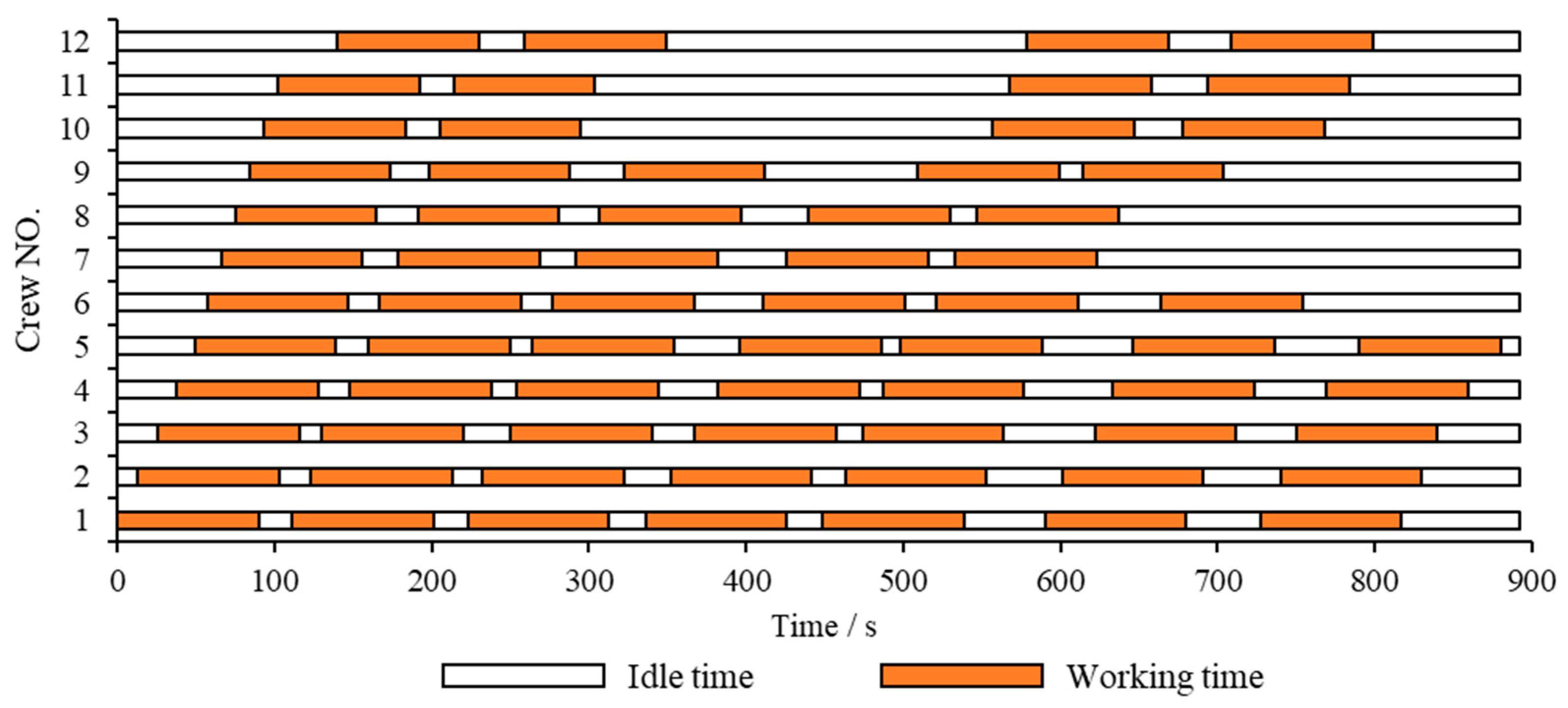
The departure time of the first bus is recorded as 0 s, and the end time of the last bus is recorded as 892s. The vehicle and charging scheme of EBs within the all-day operating hours (0–892 s) are shown in Figure 3, the vehicle-scheduling scheme of CBs is shown in Figure 4, and the crew-scheduling scheme is shown in Figure 5. In the Gantt charts below, white represents the idle time of the bus or driver, yellow indicates the service time of the mixed fleet on the route, green slashes are the charging time of EB, and orange shows the driver’s working time.
3.3. Analysis
In this section, we further analyze the optimization results in Section 3.2 in terms of two aspects: the vehicle- and charging-scheduling scheme and the crew-scheduling scheme.
- (i)
- Vehicle- and charging-scheduling scheme
Table 3 and Table 4 show the daily operation of the EB fleet and the CB fleet, respectively. Total idle time is the sum of the idle time between the first and last service trips assigned to buses. The first five EBs need to run seven service trips per day, and the sixth EB needs to run six service trips per day. The remaining EBs need to run five service trips per day. There is little difference in service intensity between different EBs. The first six EBs need to be arranged with charging trips, and the charging arrangements are shown in Table 5. Charging trips are mainly concentrated between 15:00–16:30, which belong to Period 3. The remaining battery power of EB fleet is sufficient in Period 1 and the service trips are compact, so it is difficult to recharge. Compared with Periods 2 and 4, electricity price in Period 3 is cheaper. Thus, arranging charging trips for the EB fleet in time Period 3 can save the operation cost of the EB fleet while ensuring normal operation and service integrity.
The utilization intensity of EBs is greater than that of CBs, as not only is the number of service trips allocated per day significantly larger than that of CBs, but also the idle time is less than that of CBs. CBs only need to run four trips a day, mainly distributed in 7:20–10:10 in the morning and 15:00–17:40 in the afternoon. Observing the departure timetable, it can be found that the bus route has a smaller departure interval between 7:20 and 10:10 in the morning, and hence more buses are required at the same time. As shown in Figure 3, some EBs are arranged with a charging trip from 15:00 to 17:40 in the afternoon, and the remaining EBs are not enough to ensure the normal operation of the route. In conclusion, CBs are complementary to EBs and will only be allocated service trips in scenarios where EBs are not sufficient. This is because the vehicle-scheduling problem of mixed fleets usually aims to minimize the total daily operation costs of the fleet and the economic cost of carbon emissions, and the same is true for the proposed upper-level optimization model. In the case of charging during the day (the electricity price during the day is slightly higher than that at night), the average energy consumption cost per unit mileage of the electric bus is 0.49 RMB/km. However, the fuel cost per mileage of CBs is 4.82 RMB/km, and there is an additional carbon emission cost, which is about 9.8 times that of EBs.
- (ii)
- Crew scheduling
A total of 12 drivers are required throughout the day in the one-driver-one-bus mode. Table 6 shows the daily working arrangements of drivers numbered 1 to 9. These drivers check in and check out once per day and implement a one-shift or single-shift system. Table 7 shows the daily working arrangements of the drivers numbered 10–12. These three drivers check in twice per day and check out twice per day, and a combination of the morning shift and evening shift is implemented. The fifth driver has two continuous driving trip chains, and each time, he drives two service trips continuously. The rest time between adjacent trips in two continuous driving trip chains is 14 min and 12 min, respectively, less than 15 min. Therefore, after the end of the continuous driving behavior, two longer rest time periods are arranged, which are 42 min and 58 min, respectively, greater than the prescribed 30 min. The remaining drivers do not have the continuous driving trip chain. The time feasibility constraint for the vehicle-scheduling problem focuses on the total travel time including the dwell time at the departure station, so in the one-driver-one-bus mode, drivers can take a reasonable rest by taking advantage of the dwell time at the departure station, the idle time between adjacent service trips, and the charging time of EB to avoid fatigue driving.
There are differences in total effective working hours and on-duty time between drivers, resulting in slight differences in daily wages. In order to ensure the stability and fairness of drivers’ long-term work income, shifts can be carried out in a two-week cycle. In detail, if a certain driver executes the crew-scheduling scheme in the first row in Table 6 one day, this driver will execute the scheme in the second row in Table 6 the next day, and so on.
4. Conclusions
In this study, we address the problem of collaborative scheduling of vehicles and drivers on a bus route that combines electric buses and conventional buses, with the objective of minimizing the operation costs and economic cost of carbon emissions of the mixed fleet, driver wages, and maximizing bus–driver specificity. Taking into account the service trips and charging trips performed by each bus, the bus type, and driving trips performed by each driver as the optimization variables, a bi-level multi-objective programming model is established, and the improved multi-objective particle swarm algorithm based on -constraint processing mechanism is used to solve it. Finally, an actual bus route is taken as an example to verify and validate the model. The conclusions are as follows:
- (i)
- The collaborative optimization method of vehicle scheduling and crew scheduling established for the mixed fleet can ensure the specificity of drivers and buses, and it also arranges the charging plan during valley-peak periods to ensure service integrity and save the operation cost of the bus route.
- (ii)
- The utilization intensity of EBs is greater than that of CBs, which is reflected in that not only is the number of service trips allocated each day significantly larger than that of CBs, but also the idle time is less than that of CBs. In the vehicle-scheduling process of the mixed fleet, CBs supplement EBs, and the service trip is allocated only when the number of EBs is insufficient.
- (iii)
- In the collaborating process of vehicle scheduling and driver scheduling for the mixed fleet, drivers can use the dwell time at the departure station, the idle time between adjacent service trips, and the charging time of EB to allow for reasonable rest. In this way, fatigue driving can be effectively avoided.
However, there are still some limitations in the research, which can be further discussed and studied in the future: (i) When the number of charging piles in the charging depot is limited, the vehicle-scheduling model needs to increase constraints and consider the impact of EBs queuing time on the charging duration and the remaining battery power at the end of any service trip. This will lead to the vehicle-scheduling problem becoming very complicated, and new ways of defining optimization variables will be needed. (ii) Reducing the daily utilization intensity of CBs can indeed effectively reduce the operation costs and carbon emissions of bus routes, but it will also affect the depreciation of CBs and EBs, which in turn affects the electrification process of bus routes. Therefore, in the future, extended research should be conducted on the scheduling problem of urban bus routes with limited charging depot capacity and clear electrification goals from the perspective of the whole life cycle.
Author Contributions
Conceptualization, J.W., H.W., and A.C.; and methodology, J.W. and H.W.; validation, A.C., and C.S.; investigation, J.W.; writing—original draft preparation, J.W. and A.C.; writing—review and editing, H.W.; visualization, C.S.; supervision, A.C. All authors have read and agreed to the published version of the manuscript.
Funding
This research received no external funding.
Institutional Review Board Statement
Not applicable.
Informed Consent Statement
Not applicable.
Data Availability Statement
The data presented in this study are available on request from the corresponding author.
Conflicts of Interest
The authors declared that they have no conflict of interest to this work.
Appendix A

Table A1.
Description of the main notation used in the mathematical model.
| Notation | Description |
|---|---|
| 1 if service trips i and j are adjacent trips run by EB k; 0 otherwise | |
| 1 if service trips i and j are adjacent trips run by CB h; 0 otherwise | |
| 1 if the driver g drives EB k to complete the service trip i; 0 otherwise | |
| 1 if the driver g drives CB h to complete the service trip i; 0 otherwise | |
| 1 if EB k is charged during charging trip r; 0 otherwise | |
| 1 if driver g continuously performs driving trips i and j; 0 otherwise | |
| OCB | the operation cost of CBs |
| OEB | the operation cost of EBs |
| MCB | the carbon emission of the mixed fleet |
| CP | the driver’s one-day wage |
| the variance of the number of possible vehicle swaps of drivers | |
| the number of drivers required for daily operations | |
| the number of buses that driver g needs to drive every day | |
| the fuel cost per mileage | |
| the average carbon emission per kilometer | |
| the trip length | |
| ) | departure times of service trips i (j) run by CB h |
| ) | departure times of service trips i (j) run by EB k |
| ) | the travel time of CB h on service trip i (j) |
| ) | the travel time of EB k on the service trip i (j) |
| the effective working hours of CB h on driving trip i | |
| the effective working hours of EB k on driving trip i | |
| dwell times of CB h on service trip i | |
| dwell times of EB k on service trip i | |
| the charging time of EB k on charging trip r | |
| the unit electricity price of charging in the period q | |
| the rated battery capacity of EB k | |
| the remaining battery power when EB k ends the service trip j | |
| the energy consumption of EB k on the service trip j | |
| the lower limit of the battery state of charge (SOC) | |
| the upper limit of the battery state of charge (SOC) | |
| the maximum time that the driver shall drive continuously | |
| the minimum rest time after continuous driving | |
| the maximum time that the driver work overtime |
References
- Ahani, P.; Arantes, A.; Melo, S. A portfolio approach for optimal fleet replacement toward sustainable urban freight transportation. Transp. Res. Part D Transp. Environ. 2016, 48, 357–368. [Google Scholar] [CrossRef]
- Transport for London Bus Fleet Now Meet ULEZ Standards. 300 E-Buses Expected in 2021. Available online: https://www.sustainable-bus.com/news/transport-for-london-ulez-standard-electric-buses (accessed on 14 January 2021).
- Sclar, R.; Werthmann, E.; Orbea, J.; Siqueira, E.; Tavares, V.; Pinheiro, B.; Albuquerque, C.; Castellanos, S. The Future of Urban Mobility: The case for electric bus deployment in Bogotá. Colombia 2020, 3. Available online: https://urbantransitions.global/wp-content/uploads/2020/04/The_Future_of_Urban_Mobility_web_FINAL.pdf (accessed on 12 March 2022).
- Rodrigues, A.; Seixas, S. Battery-electric buses and their implementation barriers: Analysis and prospects for sustainability. Sustain. Energy Technol. Assess. 2022, 51, 101896. [Google Scholar] [CrossRef]
- Rinaldi, M.; Picarelli, E.; D’Ariano, A.; Viti, F. Mixed-fleet single-terminal bus scheduling problem: Modelling, solution scheme and potential applications. Omega 2020, 96, 102070. [Google Scholar] [CrossRef]
- Desrochers, M.; Soumis, F. A Column Generation Approach to the Urban Transit Crew Scheduling Problem. Transp. Sci. 1989, 23, 1–13. [Google Scholar] [CrossRef] [Green Version]
- Ceder, A. Public-transport vehicle scheduling with multi vehicle type. Transp. Res. Part C Emerg. Technol. 2011, 19, 485–497. [Google Scholar] [CrossRef]
- Haghani, A.; Banihashemi, M. Heuristic approaches for solving large-scale bus transit vehicle scheduling problem with route time constraints. Transp. Res. Part A-Policy Pract. 2002, 36, 309–333. [Google Scholar] [CrossRef]
- Wang, S.; Wei, Z.; Bie, Y.; Wang, K.; Diabat, A. Mixed-integer second-order cone programming model for bus route clustering problem. Transp. Res. Part C Emerg. Technol. 2019, 102, 351–369. [Google Scholar] [CrossRef]
- Bie, Y.; Tang, R.; Wang, L. Bus Scheduling of Overlapping Routes with Multi-Vehicle Types Based on Passenger OD Data. IEEE Access 2020, 8, 1406–1415. [Google Scholar] [CrossRef]
- Tang, X.D.; Lin, X.; He, F. Robust scheduling strategies of electric buses under stochastic traffic conditions. Transp. Res. Part C-Emerg. Technol. 2019, 105, 163–182. [Google Scholar] [CrossRef]
- Bie, Y.; Xiong, X.; Yan, Y.; Qu, X. Dynamic headway control for high-frequency bus line based on speed guidance and intersection signal adjustment. Comput.-Aided Civ. Infrastruct. Eng. 2020, 35, 4–25. [Google Scholar] [CrossRef]
- Zhang, L.; Wang, S.; Qu, X. Optimal electric bus fleet scheduling considering battery degradation and non-linear charging profile. Transp. Res. Part E-Logist. Transp. Review 2021, 154, 102445. [Google Scholar] [CrossRef]
- Bie, Y.; Ji, J.; Wang, X.; Qu, X. Optimization of electric bus scheduling considering stochastic volatilities in trip travel time and energy consumption. Comput.-Aided Civ. Infrastruct. Eng. 2021, 36, 1530–1538. [Google Scholar] [CrossRef]
- Zhou, G.J.; Xie, D.F.; Zhao, X.M.; Lu, C.R. Collaborative Optimization of Vehicle and Charging Scheduling for a Bus Fleet Mixed with Electric and Traditional Buses. IEEE Access 2020, 8, 8056–8072. [Google Scholar] [CrossRef]
- Li, L.; Lo, H.K.; Xiao, F. Mixed bus fleet scheduling under range and refueling constraints. Transp. Res. Part C Emerg. Technol. 2019, 104, 443–462. [Google Scholar] [CrossRef]
- Ayman, A.; Sivagnanam, A.; Wilbur, M.; Pugliese, P.; Dubey, A.; Laszka, A. Data-Driven Prediction and Optimization of Energy Use for Transit Fleets of Electric and ICE Vehicles. ACM Trans. Internet Technol. 2022, 22, 1–29. [Google Scholar] [CrossRef]
- Lu, T.; Yao, E.; Zhang, Y.; Yang, Y. Joint Optimal Scheduling for a Mixed Bus Fleet under Micro Driving Conditions. IEEE Trans. Intell. Transp. Syst. 2021, 22, 2464–2475. [Google Scholar] [CrossRef]
- Duan, M.; Qi, G.; Guan, W.; Lu, C.; Gong, C. Reforming mixed operation schedule for electric buses and traditional fuel buses by an optimal framework. IET Intell. Transp. Syst. 2021, 15, 1287–1303. [Google Scholar] [CrossRef]
- Smith, B.M.; Wren, A. A Bus Crew Scheduling System Using a Set Covering Formulation. Transp. Res. Part A-Policy Pract. 1988, 22, 97–108. [Google Scholar] [CrossRef]
- Chen, M.M.; Niu, H.M. A Model for Bus Crew Scheduling Problem with Multiple Duty Types. Discret. Dyn. Nat. Soc. 2012, 2012, 649213. [Google Scholar] [CrossRef] [Green Version]
- Ma, J.H.; Ceder, A.; Yang, Y.; Liu, T.; Guan, W. A case study of Beijing bus crew scheduling: A variable neighborhood-based approach. J. Adv. Transp. 2016, 50, 434–445. [Google Scholar] [CrossRef]
- Ma, J.H.; Song, C.Y.; Ceder, A.; Liu, T.; Guan, W. Fairness in optimizing bus-crew scheduling process. PLoS ONE 2017, 12, e0187623. [Google Scholar] [CrossRef] [PubMed]
- Kang, L.J.; Chen, S.K.; Meng, Q. Bus and driver scheduling with mealtime windows for a single public bus route. Transp. Res. Part C-Emerg. Technol. 2019, 101, 145–160. [Google Scholar] [CrossRef]
- Lin, D.Y.; Juan, C.J.; Chang, C.C. A Branch-and-Price-and-Cut Algorithm for the Integrated Scheduling and Rostering Problem of Bus Drivers. J. Adv. Transp. 2020, 2020, 3153201. [Google Scholar] [CrossRef]
- Rahman, A.; Shibghatullah, A.S.; Abas, Z.A.; Eldabi, T.; Mon, C.S.; Hussin, A.A.A. Solving Late for Relief Event in Bus Crew Rescheduling Using Multi Agent System. J. Eng. Sci. Technol. 2020, 15, 1972–1983. [Google Scholar]
- Perumal, S.S.G.; Larsen, J.; Lusby, R.M.; Riis, M.; Christensen, T.R.L. A column generation approach for the driver scheduling problem with staff cars. Public Transp. 2021, 34. [Google Scholar] [CrossRef]
- Boyer, V.; Ibarra-Rojas, O.J.; Rios-Solis, Y.A. Vehicle and Crew Scheduling for Flexible Bus Transportation Systems. Transp. Res. Part B-Methodol. 2018, 112, 216–229. [Google Scholar] [CrossRef]
- Amberg, B.; Amberg, B.; Kliewer, N. Robust Efficiency in Urban Public Transportation: Minimizing Delay Propagation in Cost-Efficient Bus Driver Schedules. Transp. Sci. 2019, 53, 89–112. [Google Scholar] [CrossRef]
- Simoes, E.M.L.; Batista, L.D.; Souza, M.J.F. A Matheuristic Algorithm for the Multiple-Depot Vehicle and Crew Scheduling Problem. IEEE Access 2021, 9, 155897–155923. [Google Scholar] [CrossRef]
- Andrade-Michel, A.; Rios-Solis, Y.A.; Boyer, V. Vehicle and reliable driver scheduling for public bus transportation systems. Transp. Res. Part B-Methodol. 2021, 145, 290–301. [Google Scholar] [CrossRef]
- Perumal, S.S.G.; Dollevoet, T.; Huisman, D.; Lusby, R.M.; Larsen, J.; Riis, M. Solution approaches for integrated vehicle and crew scheduling with electric buses. Comput. Oper. Res. 2021, 132, 105268. [Google Scholar] [CrossRef]
- Bie, Y.; Gong, X.; Liu, Z. Time of day intervals partition for bus schedule using GPS data. Transp. Res. Part C Emerg. Technol. 2015, 60, 443–456. [Google Scholar] [CrossRef]
- Kraiem, H.; Flah, A.; Mohamed, N.; Alowaidi, M.; Bajaj, M.; Mishra, S.; Sharma, N.K.; Sharma, S.K. Increasing Electric Vehicle Autonomy Using a Photovoltaic System Controlled by Particle Swarm Optimization. IEEE Access 2021, 9, 72040–72054. [Google Scholar] [CrossRef]
- Kraiem, H.; Aymen, F.; Yahya, L.; Trivino, A.; Alharthi, M.; Ghoneim, S.S.M. A Comparison between Particle Swarm and Grey Wolf Optimization Algorithms for Improving the Battery Autonomy in a Photovoltaic System. Appl. Sci. 2021, 11, 7732. [Google Scholar] [CrossRef]
- Aymen, F. Internal Fuzzy Hybrid Charger System for a Hybrid Electrical Vehicle. J. Energy Resour. Technol.-Trans. ASME. 2018, 140, 012003. [Google Scholar] [CrossRef]
- Deb, K.; Pratap, A.; Agarwal, S.; Meyarivan, T. A fast and elitist multiobjective genetic algorithm: NSGA-II. IEEE Trans. Evol. Comput. 2002, 6, 182–197. [Google Scholar] [CrossRef] [Green Version]
Figure 1.
The overall structure of the methodology.

Figure 2.
Circular bus route layout.

Figure 3.
Vehicle and charging scheme of EBs.

Figure 4.
Vehicle-scheduling scheme of CBs.

Figure 5.
Crew-scheduling scheme.

Table 1.
Timetable of bus route.
| i | i | i | i | ||||
|---|---|---|---|---|---|---|---|
| 1 | 05:50 | 18 | 08:37 | 35 | 11:42 | 52 | 15:18 |
| 2 | 06:03 | 19 | 08:49 | 36 | 11:57 | 53 | 15:29 |
| 3 | 06:16 | 20 | 09:01 | 37 | 12:12 | 54 | 15:40 |
| 4 | 06:28 | 21 | 09:08 | 38 | 12:26 | 55 | 15:51 |
| 5 | 06:39 | 22 | 09:15 | 39 | 12:41 | 56 | 16:04 |
| 6 | 06:47 | 23 | 09:24 | 40 | 12:56 | 57 | 16:12 |
| 7 | 06:56 | 24 | 09:33 | 41 | 13:10 | 58 | 16:23 |
| 8 | 07:05 | 25 | 09:42 | 42 | 13:19 | 59 | 16:36 |
| 9 | 07:14 | 26 | 10:00 | 43 | 13:33 | 60 | 16:54 |
| 10 | 07:23 | 27 | 10:04 | 44 | 13:44 | 61 | 17:08 |
| 11 | 07:32 | 28 | 10:09 | 45 | 13:57 | 62 | 17:24 |
| 12 | 07:41 | 29 | 10:14 | 46 | 14:08 | 63 | 17:39 |
| 13 | 07:53 | 30 | 10:27 | 47 | 14:19 | 64 | 17:57 |
| 14 | 08:00 | 31 | 10:42 | 48 | 14:31 | 65 | 18:10 |
| 15 | 08:10 | 32 | 10:57 | 49 | 14:43 | 66 | 18:20 |
| 16 | 08:18 | 33 | 11:12 | 50 | 14:57 | 67 | 18:39 |
| 17 | 08:30 | 34 | 11:26 | 51 | 15:07 | 68 | 19:00 |
Table 2.
TOU power price of the general industry.
| q | Period Starting Time | Period Ending Time | (RMB/kWh) |
|---|---|---|---|
| 1 | 7:00 | 10:00 | 0.832 |
| 2 | 10:00 | 15:00 | 1.322 |
| 3 | 15:00 | 18:00 | 0.832 |
| 4 | 18:00 | 21:00 | 1.322 |
| 5 | 21:00 | 23:00 | 0.832 |
| 6 | 23:00 | 7:00 | 0.369 |
Table 3.
EB fleet daily operating arrangements.
| k | Departure Time of the First Service Trip | End Time of the Last Service Trip | Total Idle Time (min) | Total Service Time (min) | Number of Service Trips |
|---|---|---|---|---|---|
| 1 | 5:50 | 19:39 | 83 | 714 | 7 |
| 2 | 6:03 | 19:52 | 111 | 714 | 7 |
| 3 | 6:16 | 20:02 | 98 | 714 | 7 |
| 4 | 6:28 | 20:21 | 107 | 714 | 7 |
| 5 | 6:39 | 20:42 | 115 | 714 | 7 |
| 6 | 6:47 | 18:36 | 71 | 612 | 6 |
| 7 | 6:56 | 16:25 | 59 | 510 | 5 |
| 8 | 7:05 | 16:39 | 64 | 510 | 5 |
| 9 | 7:14 | 17:46 | 122 | 510 | 5 |
Table 4.
CB fleet daily operating arrangements.
| h | Departure Time of the First Service Trip | End Time of the Last Service Trip | Total Idle Time (min) | Total Service Time (min) | Number of Service Trips |
|---|---|---|---|---|---|
| 1 | 7:23 | 18:50 | 279 | 408 | 4 |
| 2 | 7:32 | 19:06 | 286 | 408 | 4 |
| 3 | 8:10 | 19:21 | 263 | 408 | 4 |
Table 5.
EB fleet charging arrangements.
| k | Departure Time of the Charging | End Time of the Charging | Charging Time (min) | Idle Time until Next Service Trip (min) |
|---|---|---|---|---|
| 1 | 15:01 | 15:33 | 32 | 6 |
| 2 | 15:15 | 15:47 | 32 | 4 |
| 3 | 15:26 | 15:58 | 32 | 14 |
| 4 | 15:39 | 16:11 | 32 | 12 |
| 5 | 15:50 | 16:22 | 32 | 14 |
| 6 | 16:13 | 16:28 | 15 | 26 |
Table 6.
Daily working arrangements of drivers 1–9.
| g | Check-in Time | Check-out Time | Total Effective Working Time (min) | Total Rest Time (min) | On-Duty Time (min) |
|---|---|---|---|---|---|
| 1 | 5:50 | 19:39 | 420 | 187 | 817 |
| 2 | 6:03 | 19:52 | 420 | 187 | 817 |
| 3 | 6:16 | 20:02 | 420 | 184 | 814 |
| 4 | 6:28 | 20:21 | 420 | 191 | 821 |
| 5 | 6:39 | 20:42 | 420 | 201 | 831 |
| 6 | 6:47 | 18:36 | 360 | 157 | 697 |
| 7 | 6:56 | 16:25 | 300 | 107 | 557 |
| 8 | 7:05 | 16:39 | 300 | 112 | 562 |
| 9 | 7:14 | 17:46 | 300 | 170 | 620 |
Table 7.
Daily working arrangements of drivers 10–12.
| g | First Check-in Time | First Check-out Time | Second Check-in Time | Second Check-out Time | Total Effective Working Time (min) | Total Rest Time (min) | On-Duty Time (min) |
|---|---|---|---|---|---|---|---|
| 10 | 7:23 | 10:57 | 15:07 | 18:50 | 240 | 53 | 413 |
| 11 | 7:32 | 11:06 | 15:18 | 19:06 | 240 | 58 | 418 |
| 12 | 8:10 | 11:51 | 15:29 | 19:21 | 240 | 69 | 429 |
Publisher’s Note: MDPI stays neutral with regard to jurisdictional claims in published maps and institutional affiliations. |
© 2022 by the authors. Licensee MDPI, Basel, Switzerland. This article is an open access article distributed under the terms and conditions of the Creative Commons Attribution (CC BY) license (https://creativecommons.org/licenses/by/4.0/).
Share and Cite
MDPI and ACS Style
Wang, J.; Wang, H.; Chang, A.; Song, C. Collaborative Optimization of Vehicle and Crew Scheduling for a Mixed Fleet with Electric and Conventional Buses. Sustainability 2022, 14, 3627. https://0-doi-org.brum.beds.ac.uk/10.3390/su14063627
AMA Style
Wang J, Wang H, Chang A, Song C. Collaborative Optimization of Vehicle and Crew Scheduling for a Mixed Fleet with Electric and Conventional Buses. Sustainability. 2022; 14(6):3627. https://0-doi-org.brum.beds.ac.uk/10.3390/su14063627
Chicago/Turabian StyleWang, Jing, Heqi Wang, Ande Chang, and Chen Song. 2022. "Collaborative Optimization of Vehicle and Crew Scheduling for a Mixed Fleet with Electric and Conventional Buses" Sustainability 14, no. 6: 3627. https://0-doi-org.brum.beds.ac.uk/10.3390/su14063627
Note that from the first issue of 2016, this journal uses article numbers instead of page numbers. See further details here.