
Road Asset Value Calculation Based on Asset Performance, Community Benefits and Technical Condition


Department of Construction Management, Faculty of Civil Engineering, University of Zilina, Univerzitna 8215/1, 01026 Žilina, Slovakia
*
Author to whom correspondence should be addressed.
Sustainability 2022, 14(7), 4375; https://0-doi-org.brum.beds.ac.uk/10.3390/su14074375
Submission received: 24 January 2022
/
Revised: 1 April 2022
/
Accepted: 4 April 2022
/
Published: 6 April 2022
(This article belongs to the Special Issue Sustainable Pavement Maintenance Management)
Abstract
:The article presents a comprehensive asset management method. Here presented method aims to bridge the economic approach to asset management with the technical approach to road infrastructure life cycle, namely its resilience and performance. The presented asset value calculation methods are based both on socio-economic viewpoints on community benefits of an asset, as well as the technical aspect of the technical condition and residual life calculations of a road infrastructure. In contrast to common road asset management methods, asset value is not arbitrarily annually depreciated, instead, it is exactly calculated based on pavement performance models, pavement construction fatigue and paving material properties. Road asset value calculation is based on the asset performance and the technical condition of a pavement structure and other objects. Road asset performance is defined in terms of society and road user demands put on road category and its qualitative standard. Road asset technical condition is evaluated by the procurement cost calculation and condition deterioration. Value of condition deterioration is defined by residual life expectancy based on fatigue and construction reliability of the road infrastructure. The cross-asset allocation method is used for the creation of programs for claim and allocation of funding. The aim was to increase the credibility of the road administrators with the public as they present their decisions based on road asset management, and to increase the level of acceptance for practitioners.
1. Introduction
Many road administrators are considering or actively trying to implement asset management systems. The main driver behind these initiatives is the public requirement to safeguard the investment of taxpayers. Asset management (AM) systems are inherently linked to a certain level of uncertainty created through both the asset valuation method and the infrastructure performance models. To mitigate this uncertainty, it is recommended to link asset management with well-developed component management systems, e.g., pavement management system, bridge management system, rail management system, etc. These should be based on the life cycle management principle. [1] The topics of pavement performance modelling method, calculation of residual life expectancy of pavement and bridges [2,3,4,5] are described in this article in an informative manner to provide background for the road asset value calculation method which is the main part of the article.
One of the main objectives of the asset management is the asset valuation. Asset valuation is used to calculate the current and future value of an asset. Asset management systems must be built on systems that work with robust values that can be accurately predicted. If a parameter, on which asset valuation is based, cannot be predicted throughout the asset lifecycle with a comfortable level of certainty, the accuracy of the asset management system will be too inaccurate to be of use. The precondition of reliability and completeness of data needed for a working road asset management has been pointed out in several studies. Refs. [6,7,8] Road administrators are unable to adequately build an argument for a funding increase with subjective systems or systems that arbitrarily simplify complex technical aspects of asset deterioration and structural and material fatigue. The description of the road asset value calculation method that utilizes these complex technical aspects is the main part of the article. Arbitrary or subjective guess-based expert systems used in the calculation of assets value can be viewed by the stakeholders and government authorities as unreliable or outright misleading. The asset value calculation methods described in the following chapters should produce objective funding claims and performance indicators of a road network administrator.
The road asset value calculation method described in this article was based on the first comprehensive works published simultaneously by the Organisation for Economic Co-operation and Development (OECD) and the Federal Highway Administration (FHWA) in the United States of America in 2000 [9,10]. ISO standards [11,12,13] specify basic definitions and requirements needed for the implementation of asset management. Country-specific implementation procedures follow the Highway infrastructure asset management guidance documents [14] for the United Kingdom.
It has been widely recognized that the implementation of the asset management is often an expensive and resource-intensive task [15]. Research articles [16,17,18] focused on the assessment of demands on road infrastructure in terms of investment criteria and equity analysis. In addition, as has been shown by Too [19], road network administrators need to have personnel with specialized know-how and skills in civil engineering, economics, traffic modelling and geographic information systems. Asset management implementation experience and related topics in different countries are frequently published and are a good base to identify pitfalls and best practices to supplement World Road Association (PIARC) Asset management guidelines [20] and proceedings of the World Road Congresses [21,22,23]. The presented method builds upon theoretical foundations laid out in journals [2,24], and at the PIARC World Congress in Abu Dhabi [25].
The point where the resources invested into developing reliable asset management pays off is the decision making. A comprehensive cross-sectional method—Cross-Asset Allocation (CAA) is described based on [23]. The output of the method are programs for funding requirements based on asset performance related to demands of the society and road users. It also defines requirements for an optimal fund allocation for the prevention of asset value decline of road infrastructure objects based on their technical condition. The technical condition is based on diagnostics and residual life expectancy calculation of objects such as roads, bridges, culverts, etc. Subsequently, alternatives for rehabilitation technology are evaluated with the use of the optimization decision-making methods and the benefit analyses including Cost-benefit analysis (CBA) [24,25,26,27,28]. CBA uses pavement performance models (PPM) based on degradation functions [29,30,31,32,33].
The equations for the asset value calculations and PPM were created by the authors appointed by the national road network manager. This would not have been possible without a complete road database maintained by the administrator for well over 20 years. This database contains long-term measurements of pavement serviceability and bearing capacity. This allows for the creation of degradation functions and residual service life calculations. Optimization of rehabilitation actions is based on CBA following national CBA guidelines or software solutions such as the Highway Development and Management Model (HDM-4).
2. Asset Management Principles and Rules
Asset management is subject to operational and accounting regulations of given country. For instance, in the European Union, this should be carried out following the Regulation of the European Parliament on the European system of national and regional accounts in the European Union [34]. This regulation defines road assets in the structure shown in Table 1.
Asset management is about managing a road administrator’s resources more similar to a business. This business-like approach requires adhering to the principles of the business economy during the road infrastructure asset management processes. Stakeholders (road users, taxpayers, politicians) need to be treated similar to customers with emphasis on economics and finance. That means a shift in thinking from the traditional engineering approach to approach focused on the satisfaction of customer expectations and more sustainable solutions [20].
Its definition, AM is an integrated set of processes and systems designed to achieve optimal and cost-effective use of assets over their lifetime, including needs identification, procurement, operation and development. It includes an economic and financial evaluation of comparisons between alternative investment options.
AM is a dynamic process. As assets wear out over time, their wear and tear manifest influencing the serviceability of the asset, its operational capability and the quality of service provided to the customer. These factors, in addition to the actual physical degradation that eventually leads to inevitable replacement and related replacement costs, constitute depreciation of the asset value. [35]. To prolong the asset life cycle, enable reliable planning and evaluation of resource allocation, system methods are incorporated into the asset management methodology, in particular the Pavement management system, Life cycles cost analysis, PPM, CBA and many others.
The implementation of AM within the road administrator modus operandi also requires the creation of a database system (road databank, asset inventory, etc.). Data collection storing and analysing should utilise modern technologies such as geographic information systems (GIS) and spatially enabled management systems [36].
Implementation of AM into the structure of road administrator’s organisation differs by the level of organisation’s maturity to adopt AM. Gap analysis can help to determine the position of the organisation [37].
Gap analysis can help to determine the position of the organisation, but generally, road administrators are usually required to follow these steps:
- creation of asset structure,
- implementing asset management policy,
- implementation of an asset management information system,
- creation of asset structure,
- assessment of the current state of existing assets,
- proposal of future requirements on assets, development program and resource planning,
- monitoring and evaluation of assets condition and performance and adherence to the development program,
- implementation of system solutions and measures to achieve the optimal state of assets.
3. Calculation of Asset Value
Calculation of asset value, i.e., asset valuation is the process of determining monetary value which translates infrastructure condition and its impacts on stakeholders into monetary terms as public wealth or equity. Basic asset valuation techniques are cost-based. For long-life infrastructure, this value gives a good representation of what is being spent on an asset omitting the effect of the periodic maintenance and necessary repairs on the actual condition of the asset. More advanced asset valuation methods take into account the actual value for the stakeholders in terms of their socio-economic benefits and value for actual road users. Equations (1)–(4) can be used for these advanced asset valuation techniques as road asset value of:
- Community society benefits.
- Road system performance.
The assessment of community benefits values the level of transport service available to the stakeholders. These stakeholders are road users but also the public directly affected by services provided by traffic on the valuated asset. These services include generation of capital, providing clientele to services, development of the cities and regions, and the protection of the environment.
The assessment of road system performance evaluates the road category and its capacity; it takes into account the road geometric parameters, traffic intensity, and traffic safety.
The calculation of the asset value based on its technical condition is a method similar to the Depreciated Replacement Cost (DRC) method [38]. The improvement provided by here presented method is that the depreciation is based on the exact determination of the operational serviceability and structure asset condition. The quantification of operational serviceability and structure asset condition is carried out with the use of pavement performance models and residual life expectancy, which is calculated as resistance to fatigue of pavement construction and paving materials. These advanced concepts are explained in later chapters, but the gist is that pavement operational serviceability is the ability of pavement to ensure safe and economical road traffic; residual life expectancy is the technical condition of the pavement expressed as the ability of the road to bear the traffic load.
3.1. Performance-Based Asset Value
Performance-based asset valuation means that the road assets are valued in terms of their services and socio-economic benefits to the community. These benefits are achieved by road asset performance ensuring safe and economic traffic.
Here presented methods and equations have been created by the authors. It is an excerpt from report commissioned by Ministry of Transport and Construction of Slovak republic and the Slovak Road Administration [39].
3.1.1. Value of the Community Benefits
The proposed asset value of community benefits is created by the transport services provided by the road infrastructure to the community’s wellbeing and prosperity. These services include transportation to work, travel, medical accessibility, emergency responder accessibility, communal services, etc. In addition, transportation asset availability and a certain required level of asset performance can be required to fulfil international agreements or commitments. Road asset availability and performance may also reduce environmental impacts of traffic and can help to develop a region through the attraction of investors and developers by fulfilling their logistic requirements.
The value of community benefits is produced by the mere existence of an asset and its transportation significance, but it is heavily influenced by the serviceability—traffic capacity, geometric parameters, speed restrictions, and ride quality.
The value of the community benefits of an asset is calculated by comparing its current condition against its ideal condition. The following method is recommended for the comparison:
- DRC calculation of the existing asset;
- calculation of the acquisition cost of a new asset with the ideal parameters, this may be a complex reconstruction and modernization of the existing asset or construction of a new ideal asset that will compete with the existing evaluated asset (bypass, highway alternative, etc.);
- calculation of the difference between the DRC of the evaluated existing asset and construction costs of the new ideal asset.
The proposed method should be used to forecast asset value in the future. The precondition is to be able to predict asset performance during the asset life cycle and the exact length of the life cycle by calculation of the residual service life of the road. This is elaborated in detail in later chapters. The ratio of the residual service life of the valuated asset to the theoretic service life of a new ideal asset is a coefficient that has to be used to multiply DRC of the valuated asset.
Value of community benefit is the sum of discounted annual cash flows during the evaluating period which is usually the asset life cycle. Annual cash flow is the sum of annual benefits produced by the asset improvement and the difference between the DRC and purchasing price of a new ideal asset.
The proposed calculation of the asset value of community benefits is shown in Equation (1).
NPVCB = net present value of community benefits [€],
Bt(a−b) = community benefits as a difference between scenario a—no complex reconstruction and modernization or a new asset and b—complex reconstruction and modernization or a new asset “do something” (b) in year “t” [€],
APt = acquisition price in “do something” scenario in year “t” [€],
MCt = maintenance cost increase in “do something” scenario in year “t” [€],
u = discount rate [%],
Tzp = year of the beginning of the life cycle [year],
T = evaluation of individual years of the life cycle [years].
3.1.2. Value of Road Asset Performance
The performance of a road asset has a value related to the traffic capacity, geometric parameters, speed restrictions, and ride quality. This asset performance should ensure smooth, economic, and safe traffic flow during the road life cycle.
The proposed calculation of economic efficiency is calculated the same way as described in Section 3.1.1, however, instead of community benefits, only road user costs are considered. The value of road system performance will be always lesser than the value of the community benefits since the value of the community benefits includes the value of road system performance.
NPVRSP = net present value of community benefits [€],
RUB(a−b) = road user benefits as a difference between scenario a—no complex reconstruction and modernization or a new asset and b—complex reconstruction and modernization or a new asset “do something” (b) in year “t” [€],
APt = acquisition price in “do something” scenario in year “t” [€],
MCt = maintenance cost increase in “do something” scenario in year “t” [€],
u = discount rate [%],
Tzp = year of the beginning of the life cycle [year],
T = evaluation of individual years of the life cycle [years].
These road system performance benefits are tied with the road users’ benefits and their travel time costs, vehicle operating costs, and accident costs. These costs are demands monetized for travel time, fuel costs, lubricant costs, vehicle wear, etc. Additional external environmental costs such as emissions, noise and others may be included [40].
User costs are heavily influenced by traffic intensity, geometric parameters, intersections, pavement degradation, etc. We propose that the user cost calculation before and after the recovery is performed following national CBA guidelines such as European Commission guideline [41] or software solutions such as the Highway Development and Management Model (HDM-4).
3.2. Calculation of Value Based on the Technical Condition
The technical condition of road infrastructure can be evaluated based on parameters that define a road’s operational capability, therefore, value based on technical condition can be called the technical condition value of the asset.
Operational capability is the ability of the road to perform the required operational functions. It is the condition and quality of the asset. The criteria of operational capability include road unevenness, surfacing defects, and skid resistance.
Technical condition is the ability of the road to withstand traffic loads. Technical condition is expressed as a level of wear compared to the asset’s theoretical pristine condition. For roads, this is the difference calculated as the residual bearing capacity or residual service life of pavement as described in [2,42].
3.2.1. Operation Capability Value of an Asset
The proposed operation capability value of an asset is monetarily expressed as a value of an asset’s ability to perform and fulfil services demanded by road users. Calculation of the value can follow the method described in Section 3.1. The difference is that pavement rehabilitation is considered to be an improvement of the operational capability. In this case, the “do something” doesn’t mean a start of a new life cycle or an acquisition of a new asset. The operation capability value is the sum of road user benefits during the asset’s life-cycle. The ”do something“ scenario is the maintenance and repair standard employed by the road administrator on the asset. This value serves the administrator to judge his maintenance and repair strategies and optimize them for maximal operational capability of the road asset.
The benefits are expressed as the difference between the user costs of the desired pristine condition and its present state as seen in Equation (3). Operational capability value for bridges is not calculated because the road users are affected only by the bridge pavement.
NPVOC = net present value of operational capability [€],
UCDN = total annual road user costs for “do nothing” scenario in year t [€],
UCDS = total annual road user costs for “do something” scenario in year t [€],
kDEG = degradation coefficient (incremental or absolute depending on the pavement performance model),
kGAADT = annual average daily traffic growth coefficient.
UCDN and UCDS is the annual sum of road user costs categories of all vehicle types on a road section (a road asset usually consists of several homogenous road sections) for given scenario. For maintenance and repair evaluation needed for calculation of asset operational capability value, these consumptions are best related to changes expressed by the international roughness index (IRI). Changes in road user cost can be calculated using proprietary software solutions such as HDM-4 or by simplified models where road user cost increase coefficients are derived from IRI changes as shown in Equation (4).
UCz,i,j,k = user costs of type “z” (fuel, oil, maintenance, etc.), in year “i” of vehicle type “j” on section “k” [€],
ACz,i,j,k,IRI=1 = average consumption of type “z”, in year “i” of vehicle type “j” on section “k” or IRI = 1 m ∗ km−1, [(l, hours, % tires, % cars etc.) *],
UCz,j = unit cost of type “z” for vehicles of type “j” [€*(litre, hour, tyre, car)-1],
kIRI = road user cost coefficient for IRI in the year “I”.
3.2.2. The Value of the Construction—The Technical Condition
The proposed value of the construction—technical condition, i.e., construction value is an economically expressed value related to the ability of the asset (road structure, bridge) to withstand traffic load. This value is needed exclusively for the asset manager, i.e., not the user due to optimal asset management related to the construction of the road, bridge, etc. The current value is defined by calculating the current acquisition price which is reduced by the coefficient of wear of the structure. This is expressed as a ratio of the residual life to the designed life.
AVCC = value of an asset in current technical condition [€],
AAPPC = acquisition price of the asset in a pristine condition [€],
RLE = residual life expectancy [year],
DLE = designed life expectancy [year].
The proposed calculation of the current design value of an asset in relation to the optimal value, i.e., projected life can be expressed by Equation (6).
CVR = is the ratio of the current value of the asset to the current acquisition price of the asset in pristine condition [%].
3.2.3. Degradation Calculation
The key element of the proposed asset value calculations are the PPM’s. PPM is used to mathematically express the surface properties of pavements and their deterioration in relation to road construction, climatic and traffic effects. The road user costs (see Equation (4)) are directly proportional to pavement degradation and, if everything else is being equal (traffic, maintenance, climatic conditions etc.), this holds true also for the road user benefits which make a difference between road user costs in “do something” and “do nothing” scenarios in Equations (1) and (2).
Calculation of benefits RUB(a−b) in Equation (1) and NPVOC in Equation (2) produces the difference between user costs in both scenarios over the life expectancy of the asset. However, the benefits over the course of the asset life cycle are not linear due to the changing properties of the asset’s operational capability. Therefore, it is necessary to know the course of these changes, which is possible through PPM. Knowledge of PPM thus determines the accuracy of the calculation of the asset value.
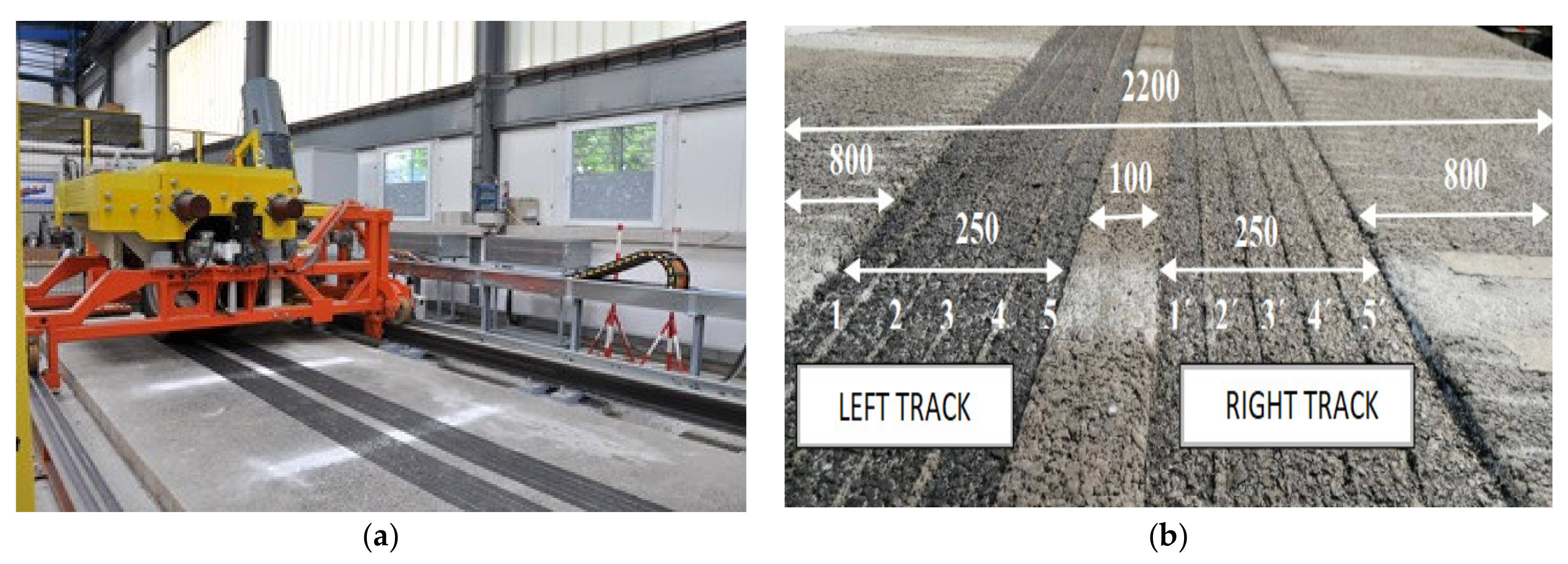
We propose that PPM should be derived either from experimental measurements on experimental sections or from long-term measurements on real pavements. For road asset managers with incomplete road data inventory, accelerated pavement testing may provide reliable PPM within the course of several months (Figure 1).
The actual pavement degradation expressed by the PPM is sometimes also called the pavement degradation model or degradation curves. Mathematically expressed degradation curves are used to describe the changes in pavement conditions during its life cycle. These mathematical functions express a relationship between changes in pavement serviceability, and the time or the number of load repetitions. The general shape of the degradation curves is usually described as an exponential function, which is a rule that gives independent variables (time or load repetitions) a value of a dependent variable (pavement serviceability parameter), see Equation (7).
P(n) = relative value of pavement serviceability parameter depending on the number of load repetitions “n”,
n = number of past load repetitions at the time of evaluation,
N = estimated total number of load repetitions until the limit value of the parameter is reached,
A = coefficient expressing the type of pavement and the types of materials used 0 <A ≤ 1,
B = exponent expressing the degradation, for individual parameters, values in interval 0.2–6.0.
At the APT experimental section, degradation curves were derived for a given type of pavement construction, climatic conditions and traffic load. Individual degradation functions were derived for the parameter of skid resistance, transverse and longitudinal unevenness.
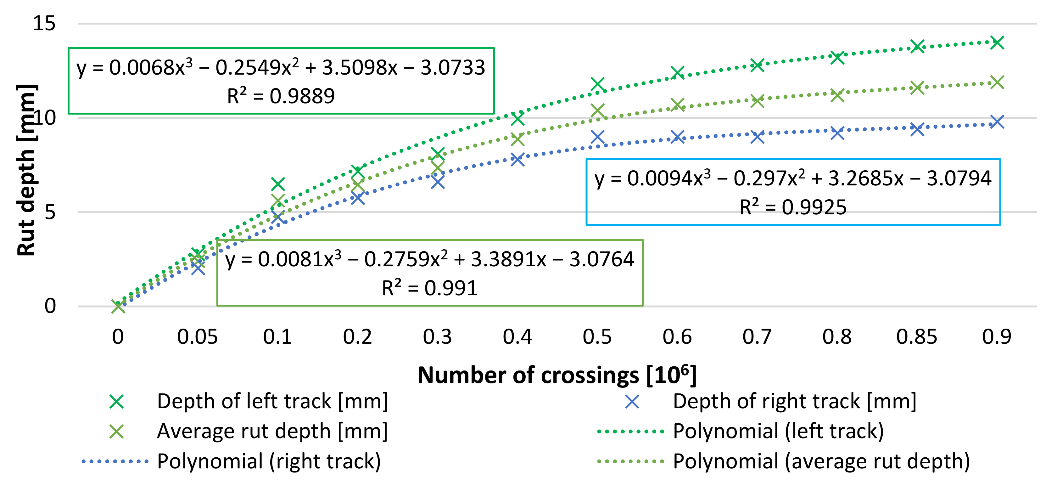
In Figure 2 there are shown three degradation functions of the Rut depth obtained experimentally by pavement operational serviceability modelling, such functions can be evaluated as dependence of Rut depth parameter in relation to number of crossings. In Figure 3 there is an evaluation of the same parameter of Rut depth as a next step of operational serviceability modelling where a growth of the Rut depth parameter is evaluated as a relative value by Equation (7). Such degradation function of Rut depth obtained from APT was already partly presented in several studies [2,43].
Road asset managers with mature and thorough road data inventories may prefer using historical data to create PPM. This is called long-term pavement performance monitoring (LTPPM). Reliability may be higher or lesser than PPM created from APT depending on the LTPPM data matrix. Loading intensity and climate conditions data are well known in APT testing, LTPPM usually provides only general estimation of these data.
As an example, we provide functions based on LTPPM of 15 years on real pavement sections monitored by the national administrator. Based on the analysis of these stored values, it was possible to mathematically derive the following functions (Equations (8)–(13)).
Longitudinal unevenness of trunk roads:
- time dependence T
y =−1.058x3 + 1.260x2 − 0.628x + 0.409
R2 = 0.961
R2 = 0.961
- load dependence N
y = −1.141x3 + 1.498x2 − 0.834x + 0.449
R2 = 0.965
R2 = 0.965
Transverse unevenness of trunk roads:
- time dependence T
y = −0.491x3 + 0.431x2 − 0.424x + 0.548
R2 = 0.973
R2 = 0.973
- load dependence N
y = −0.561x3 + 0.692x2 − 0.704x + 0.595
R2 = 0.983
R2 = 0.99
R2 = 0.983
R2 = 0.99
Skid resistance of trunk roads:
- time dependence T
y = −1.958x3 + 0.814x2 + 0.261x + 0.824
R2 = 0.955
R2 = 0.955
- load dependence N
y = 0.848x3 − 4.210x2 + 2.830x + 0.438
R2 = 0.927
R2 = 0.927
3.2.4. Calculation of the Residual Life Expectancy
The degradation of an asset at any given time during its life cycle ranges from 1.0—pristine condition to 0.0—emergency failure condition. The technical condition can be calculated as the residual life expectancy and its proportion to the projected life, see Equation (5). The calculation of the residual life expectancy itself is relatively difficult and differs for different types of assets (road, bridge, other). Similar to the calculation of degradation curves, the accuracy of the residual life expectancy calculation depends heavily on the accuracy of the input values.
Pavements
We advocate that the calculation of the residual life expectancy should be based on the methodology of pavement structure design, calculation of the current physical and deformation characteristics of pavement structure layers, and experimental measurement of fatigue characteristics of asphalt mixtures of the pavement surfacing. The basic relationship for the assessment of pavement construction is shown in Equation (14) [44].
σr,I = radial stress at the lower edge of the surfacing layer, which arises in the period “i” when loaded by the design axle [MPa],
Ri,I = calculated the value of the flexural tensile strength of the material under consideration for the conditions in period “i” [MPa],
SN = fatigue coefficient.
To use this equation for the calculation of the residual life expectancy of existing pavement, it is necessary to derive the actual modulus of elasticity and strength, especially in the surfacing layers. These are estimated during diagnostics of the pavements’ load-bearing capacity utilizing a falling weight deflectometer. [45]. FWD produces an impact on the pavement, which induces a flexible reaction. This reaction can be graphically represented by a deflection bowl. The shape of this bowl shows the deflection ordinates of individual sensors attached to the pavement. Based on the so-called back-calculation, the actual modulus of elasticity of the individual pavement layers is calculated. The back-calculation is a calculation in the layered elastic half-space model [46,47,48,49]. Subsequently, based on the modulus of elasticity, the stresses in the individual layers of the road structure are calculated.
The calculation of the residual life expectancy itself is derived based on the fatigue coefficients a and b in Equation (15). For the calculation of the fatigue coefficients, it is necessary to experimentally derive the parameters of fatigue characteristics which express pavement resilience against repeated loading. The test is carried out by repeated bending of a pavement surfacing layer test sample. Fatigue tests were carried out according to the European standard [50]. The results of the fatigue test are in the form of a Wöhler diagram shown in Figure 4.
ε0j = maximum amplitude of proportional deformation during the test conditions at the beginning of the measurement,
a,b = parameters measured during the fatigue tests is the stress lines coefficient in the range of N,
N = the number of load repetitions.
Calculation of maximum design axle load repetitions that the pavement can withstand can be determined from Equation (16).
DAL = number of design axle loads
ε6 = average deformation derived from fatigue curve after 106 loading cycles in microstrain [µm/m].
εj = calculated relative deformation on the lower fibres of the bituminous bound sub-layer in the pavement construction,
γ = fatigue test reliability factor—1.6
B = fatigue characteristics—falling gradient of the fatigue line, B = −1/b
For the implementation of this method into asset value calculation described in previous chapters, measurements were performed for the standard asphalt modified surfacing layer: AC 16 L PMB 45/80-75. The resulting shape of the deflection curve and the achieved parameters are shown in Figure 4 and Table 2. More detailed results for fatigue tests can be found in [51,52].
Where ε6 is strain level required for 1 million cycles fatigue life; b is slope parameter of fatigue line, B is falling gradient of the fatigue line, B = −1/b and A0 is value of intercept of samples related strain (log ε) and samples loading cycles count (log N).
Bridges
Systems of bridge construction condition evaluation can be divided into two groups:
- Evaluation systems based on index values—determined by mathematical-statistical operations with element evaluations and classification of their failures.
- Evaluation systems based on probabilistic calculations—calculations of the reliability of bridges concerning their load capacity and service life.
The systems differ in the degree of objectivity and complexity of the evaluation. The result of the bridge construction condition evaluation is the categorization of bridge structures into seven levels, from 1st degree—pristine condition, to 7th degree—emergency condition.
Bridges in the 7th category suffer from failures that affect the load capacity of the bridge to an extend that immediate action is required to avert the impending catastrophe.
In terms of the system approach in the bridge management system, the technical service life and residual service life are defined. The technical service life is mathematically modeled using a degradation curve, which is modified either absolutely, i.e., throughout its course, or partially, i.e., only in certain intervals. Modifications of the degradation function are given by the properties of the structure resilience, defects and failures of the structure, external influences (aggressive environment and traffic load), the level of maintenance, repairs performed, and other factors.
The modified degradation curves express the development of the particular property over time and the life expectancy is the period at the end of which the property reaches the limit of acceptable values. The modified function of the degradation curves is proposed in Equation (17).
t = bridge asset,
V0 = initial value of the bridge asset,
D(t) = degradation function,
∑mi(t) = sum of modification factors, variable or constant over time,
D0(t) = basic degradation function.
The degradation curves differ depending on the type of bridge construction. The residual life expectancy represents the modeling of the behavior of the bridge construction in time depending on its condition and the effect of the surrounding environment. The result is a prognostic model that allows for a qualified estimate of the time during which to use the bridge is still possible, i.e., meeting at least the minimum operational requirements.
Other Objects
Other objects on the road infrastructure include culverts, drainage equipment, lighting, etc. From the point of view of the information systems, they do not have decision-making optimization methods and therefore, expert guess is sufficient for determining their value. The technical condition of the object is estimated based on visual inspections or experimental diagnostic methods to determine their degree of wear compared to their pristine condition.
4. Value-Based Asset Management: Cross-Asset Allocation Method
Asset value calculation methods presented in previous chapters can produce asset values and the value of the managed road network as the sum of these values. These asset values and road network values are useful by themselves as indicators and for communication with public and government authorities. However, the greatest potential is their implementation of the value-based decision-making procedures.
The road administrator has to decide which particular value or combination of values or even sum of all values will be crucial for his decision making [53]. Community value, performance value, and technical condition value may have different importance based on culture, and administrator’s level (municipal, regional, national). Road network development and maintenance based on asset value allow for the creation of investment strategies and maintenance programs that can stabilize, optimize or maximize road network values. These programs and strategies should be based on objective fund allocation methods such as the cross-asset allocation method.
Cross-asset allocation is the decision-making process by which resources to multiple programs or asset classes are distributed based on the simultaneously quantified prioritization of utility [54].
This performance-based resource allocation can have a bottom-up or a top-down approach as described by Nicolosi [23]. Here presented method of cross-asset allocation is a top-down approach, see Figure 4. We present a novel method for calculation of a rehabilitation program action plan that allocates resources to maximize the value of assets within the road network, see Equation (11). In addition, calculation method for the maximization of the asset value when investment programs compete with rehabilitation programs. This method uses a performance index as a way to maximize the benefits of both types of individual programs.
The cross-asset allocation method based on asset value calculated by methods described in previous chapters also benefits from the added reliability provided by PPM and objective residual life expectancy calculation. The outputs of this method are investment programs and budgets for managing the value of the road network. In addition to the methods described in previous chapters, the design of new pavements, as well as the design of overlays and other rehabilitation technologies, should be based on pavement design method, life-cycle analysis, PPM, overlay thickness optimization, and CBA as described in [2,3,24,55,56].
If the road network manager is unable to secure funding to increase the value of his assets, he should aim to at least stabilize the value with the most effective investments conserving road serviceability (see programs V, M, O). These investments are usually thin overlays applied in a timely manner. These technologies don’t increase the bearing capacity, i.e., operation capability. This may be a short-term strategy as this type of rehabilitation doesn’t extend the expected residual life of a pavement. Ideally, the road network manager should have enough funds to strategically invest to increase the value of the road network. All investment programs should be created following these four basic principles:
- 1st Principle: Each asset has both a value and performance (see Section 3).
- 2nd Principle: The proposed budget claim must allow restoring the asset from its current technical condition to a normatively defined standard.
- 3rd Principle: Funds need to be claimed and allocated for all objects that are a part of the road network, this includes roads, bridges, and other objects.
- 4th Principle: The life cycle of each asset must be evaluated.
The investment programs can be split into two categories:
- Fund allocation programs to achieve the required normative technical level of asset value.
- Asset development programs based on achieving their required performance.
A schematic of a comprehensive asset management methodology including all described principles as shown in Figure 4. The outputs of the method are individual programs:
- Program—V is a list of rehabilitation works necessary to maintain assets at a level that will keep the roads in a serviceable condition.
- Program—M is a list of rehabilitation works necessary to maintain assets at a level that will keep the bridges in a serviceable condition.
- Program—O is a list of rehabilitation works necessary to maintain assets at a level that will maintain the other objects of the road network in a serviceable condition.
- Program—ICS is a list of investments that will ensure that the performance of assets meets the road network criteria.
- Program—IS is a list of investments that will ensure that the performance of assets meets society demands.
The V, O and M programs are created with the use of the pavement management system and LCCA methods. If the technical condition of the asset no longer meets the operational capability, a rehabilitation of the asset is proposed within its life cycle to extend the asset life cycle. The sum of funds needed for programs V, M and O is the minimum financial budget that the road administration needs to secure the operation of the road network and stabilize its technical condition value. The program is a repair action plan of different rehabilitation works applied across all assets of the selected road network with maximal effect within budget constrain as we propose in Equation (18).
Programs ICS and IS should provide additional funds necessary to stabilize and increase the community value and asset performance value. The sum of all programs will create the cross-sectional price.
TOb = program action plan of rehabilitation actions on the road network,
TSi = is the value of the performance criterion of asset “i” derived from the technical condition of the asset and its max. values (see Section 3) and for the case of implementation of rehabilitation technology TOi,s,
TOi,s = is a variant of rehabilitation technology “s” on an asset “i”,
Price (TOb,s) = is the price of rehabilitation technology “s” on asset “i”.
b = budget limit for program “i”
In case of limited funding, it is theoretically possible to allocate funds into ICS and IS even at the price of pulling funds from V, M and O programs [23]. However, it is necessary to introduce a strategic performance index as a combination of the advantages of individual programs, see proposed Equation (12). For instance, a lane addition on one asset to considerably increase its community and road user value may produce more value than securing serviceability on another road asset. However, the introduction of such coefficients has a subjective character and therefore the introduction of such allocation is purely theoretical. We can express this with Equation (19). The scheme of the creation of a final comprehensive cross-sectional program is shown in Figure 5.
POV = combined asset value produced by program V,
POM = combined asset value produced by program M,
POIS = combined asset value produced by program IS,
VIi = is the asset value of the performance index “i” as a linear combination of the benefits of individual programs,
Price (VIi) = complex cross-sectional price.
5. Conclusions
Arbitrary or subjective guess-based expert systems used in the calculation of assets value can be viewed by the stakeholders and government authorities as unreliable or outright misleading. Road administrators are unable to adequately build an argument for a funding increase with systems based on simplified technical aspects of asset deterioration and structural and material fatigue. The asset value calculation methods described in this paper incorporate PPM and residual service life calculation based on fatigue and rheological material properties for the prediction of asset service life. These should eliminate subjective arbitrary simplifications and should produce objective funding claims and performance indicators of the road network administrator capabilities.
The precondition to the application of these methods is an APT research program and/or an asset database with enough historical data to produce reliable PPM. The second precondition is the ability to asset pavement bearing capability and use it to calculate the residual service life of a pavement and design overlay thickness of rehabilitation actions. The application of cross-asset allocation method is recommended for the funding allocation of resources within investment programs aimed to optimize asset values described in this paper. The implementation of methods presented in this paper may require system steps within his manager’s modus operandi and organizational structure. In principle, these are the following steps:
- defining the requirements of the society and road infrastructure users from the current and long-term point of view,
- creation of the organization’s goals in terms of meeting the prospective goals-strategic plan,
- creation of method and schedule for implementation of asset management and administration,
- creation of the organizational structure of the organization taking into consideration the needs of asset management and administration,
- creation of organizational requirements, e.g., legal, financial, etc., for the implementation of asset management,
- personnel requirements of the organization for the implementation of asset management,
- assessment of the current state of assets,
- definition of alternative solutions to achieve the optimal condition of assets,
- implementation of a system for regular monitoring of the asset condition, i.e., controlling,
- defining the risks relevant to the realization of the organization’s asset management objectives.
In terms of these recommendations, it is realistic to successfully implement asset management systems based on the methods and algorithms described above. This will create the preconditions for a modern asset management system and optimally increase the value of road infrastructure and available funds.
Author Contributions
J.M. was in charge of the research, he coordinated and provided an oversight over all stages of the research. M.K. participated in preparation of the draft. Ľ.R. lead the APT research and coordinated the research team and wrote the article. M.K. compiled LTPPM data and created the presented pavement performance model, he also contributed to the final manuscript. All authors have read and agreed to the published version of the manuscript.
Funding
This research received no external funding.
Institutional Review Board Statement
Not applicable.
Informed Consent Statement
Not applicable.
Data Availability Statement
The data that are presented in this study are available within the figures and tables. They are also available from the corresponding author upon request.
Conflicts of Interest
The funders had no role in the design of the study; in the collection, analyses, or interpretation of data; in the writing of the manuscript, or in the decision to publish the results.
References
- Cowe Falls, L.; Haas, R.; McNeil, S.; Tighe, S. Asset Management and Pavement Management: Using Common Elements to Maximize Overall Benefits. Transp. Res. Rec. 2001, 1769, 1–9. [Google Scholar] [CrossRef]
- Mikolaj, J.; Remek, L.; Kozel, M. Optimization of Life Cycle Extension of Asphalt Concrete Mixtures in Regard to Material Properties, Structural Design and Economic Implications. Adv. Mater. Sci. Eng. 2016, 2016, 6158432. [Google Scholar] [CrossRef] [Green Version]
- Mikolaj, J.; Schlosser, F.; Remek, L.; Chytcakova, A. Asphalt Concrete Mixtures: Requirements with Regard to Life Cycle Assessment. Adv. Mater. Sci. Eng. 2015, 2015, 567238. [Google Scholar] [CrossRef] [Green Version]
- Maaty, A. Temperature Change Implications for Flexible Pavement Performance and Life. Int. J. Transp. Eng. Technol. 2017, 3, 1–11. [Google Scholar] [CrossRef] [Green Version]
- Xiao, D.; Qiu, Y.; Wang, K.C. Mechanistic-empirical pavement design guide (MEPDG): A bird’s-eye view. J. Mod. Transp. 2013, 19, 114–133. [Google Scholar] [CrossRef] [Green Version]
- Van der Velde, J.; Klatter, L.; Bakker, J. A holistic approach to asset management in the Netherlands. Struct. Infrastruct. Eng. 2013, 9, 340–348. [Google Scholar] [CrossRef]
- Brint, A.; Black, M. Improving estimates of asset condition using historical data. J. Oper. Res. Soc. 2014, 65, 242–251. [Google Scholar] [CrossRef]
- Migliaccio, G.; Bogus, S.; Cordova-Alvidrez, A. Continuous Quality Improvement Techniques for Data Collection in Asset Management Systems. J. Constr. Eng. Manag. 2014, 140, B4013008. [Google Scholar] [CrossRef]
- Organisation for Economic Co-Operation and Development (OECD). Asset Management for the Roads Sector; Road Transport and Intermodal Linkages Research Programme; OECD Publishing: Paris, France, 2001. [Google Scholar] [CrossRef]
- U.S. Department of Transportation. Department of Transportation. Asset Management Primer; Federal Highway Administration, Office of Asset Management: Washington, DC, USA, 1999; p. 30. [Google Scholar]
- ISO 55000; Asset Management—Overview, Principles and Terminology. 1st ed. National Standards Institute (ANSI): Washington, DC, USA, 2014; pp. 1–26ISBN 978-9267107110.
- ISO 55001; Asset Management—Management Systems—Requirements. 1st ed. National Standards Institute (ANSI): Washington, DC, USA, 2014; pp. 1–24ISBN 978-9267107448.
- ISO 55002; Asset Management—Management Systems—Guidelines for the Application of ISO 55001. 2nd ed. National Standards Institute (ANSI): Washington, DC, USA, 2018; pp. 1–84ISBN 978-9267110066.
- UK Roads Liaison Group. Highway Infrastructure Asset Management; Guidance Document; Queen’s Printer and Controller of Her Majesty’s Stationery Office: London, UK, 2013; p. 119. [Google Scholar]
- Godau, R. Why asset management should be a corporate function. J. Public Work. Infrastruct. 2008, 1, 171–184. [Google Scholar]
- Premius, H. The Infrastructure We Ride on. Decision Making in Transportation Investment. Transp. Rev. 2019, 39, 560–562. [Google Scholar] [CrossRef]
- Jafino, B.A.; Kwakkel, J.; Verbraeck, A. Transport network criticality metrics: A comparative analysis and a guideline for selection. Transp. Rev. 2020, 40, 241–264. [Google Scholar] [CrossRef]
- Di Ciommo, F.; Shiftan, Y. Transport equity analysis. Transp. Rev. 2017, 37, 139–151. [Google Scholar] [CrossRef] [Green Version]
- Too, E. Infrastructure asset: Developing maintenance management capability. Facilities 2012, 30, 234–253. [Google Scholar] [CrossRef] [Green Version]
- Piarc Asset Management Manual: A Guide for Practitioners. Available online: https://road-asset.piarc.org/en (accessed on 1 March 2022).
- Kokot, D. Common Framework for a European Life, Cycle Based Asset Management Approach for Transport Infrastructure Networks. Routes/Roads 2019, 2, 27–29. [Google Scholar]
- AM4INFRA. 2018. Available online: www.am4infra.eu (accessed on 13 November 2020).
- Nicolosi, V. Multi–Objective Approaches to Cross-Asset Resource Allocation in Transportation Asset Management. Routes/Roads 2019, 38, 37–44. [Google Scholar]
- Mikolaj, J.; Remek, L.; Macula, M. Asphalt concrete overlay optimization based on pavement performance models. Adv. Mater. Sci. Eng. 2017, 2017, 6063508. [Google Scholar] [CrossRef] [Green Version]
- Mikolaj, J.; Remek, L. Utilization of new methods for road infrastructure asset management in Slovakia. In Proceedings of the 26th World Road Congress, Abu Dhabi, United Arab Emirates, 6–10 October 2019; pp. 1–15. [Google Scholar]
- Life-Cycle Cost Analysis Procedures Manual: State of California Department of Transportation Division of Maintenance Pavement Program. 2013. Available online: https://dot.ca.gov/-/media/dot-media/programs/maintenance/documents/office-of-concrete-pavement/life-cycle-cost-analysis/lcca-25ca-manual-final-aug-1-2013-v2-a11y.pdf (accessed on 1 March 2022).
- Dayong, W.; Changwei, Y.; Kumfer, W.; Hongchao, L. A life-cycle optimization model using semi-markov process for highway bridge maintenance. Appl. Math. Model. 2017, 43, 45–60. [Google Scholar] [CrossRef]
- Mandapaka, V.; Basheer, I.; Khushminder, S.; Udloitz, P.; Harvey, J.T.; Sivaneswaran, N. Mechanistic-Empirical and Life-Cycle Cost Analysis for Optimizing Flexible Pavement Maintenance and Rehabilitation. J. Transp. Eng. 2012, 138, 625–633. [Google Scholar] [CrossRef]
- Gong, H.; Sun, Y.; Shu, X. Use of random forests regression for predicting IRI of asphalt pavements. Constr. Build. Mater. 2018, 189, 890–897. [Google Scholar] [CrossRef]
- Gupta, A.; Kumar, P.; Rastogi, R. Critical Review of Flexible Pavement Performance Models. J. Civ. Eng. 2014, 18, 142–148. [Google Scholar] [CrossRef]
- Susanna, A.; Crispino, M.; Giustozzi, F.; Toraldo, E. Deterioration trends of asphalt pavement friction and roughness from medium-term surveys on major Italian roads. Int. J. Pavement Res. Technol. 2017, 10, 421–433. [Google Scholar] [CrossRef]
- Wu, K. Development of PCI-Based Pavement Performance Model for Management of Road Infrastructure System; Arizona State University: Arizona, AZ, USA, 2015; Available online: https://repository.asu.edu/attachments/163996/content/Wu_asu_0010N_15506.pdf (accessed on 29 June 2021).
- Ferreira, A. Selection of pavement performance models for use in the Portuguese PMS. Int. J. Pavement Eng. 2011, 12, 87–97. [Google Scholar] [CrossRef]
- European Committee. Regulation of the European Parliement and of the Concil on the European System of National and Regional Accounts in the European Union; European Committee: Brussels, Belgium, 2010; Available online: https://www.europarl.europa.eu/RegData/docs_autres_institutions/commission_europeenne/com/2010/0774/COM_COM(2010)0774_EN.pdf (accessed on 20 January 2022).
- American Association of State Highway and Transportation Officials (AASHTO). AASHTO Transportation Asset Management Guide (Executive summary); Report Number: FHWA-HIF-13-047; American Association of State Highway and Transportation Officials: Washington, DC, USA, 2013. Available online: https://www.fhwa.dot.gov/asset/pubs/hif13047.pdf (accessed on 20 January 2022).
- Institute of Asset Management. Asset Management—An Anatomy; Version 3; Institute of Asset Management: Bristol, UK, 2015; Available online: https://theiam.org/media/1486/iam_anatomy_ver3_web-3.pdf (accessed on 21 January 2022).
- Scott, R.; Plano, C.; Nesbitt, M. Transportation Performance Management Capability Maturity Model; U.S. Department of Transportation, Federal Highway Administration Office of Transportation Performance Management: Washington, DC, USA, 2016; Available online: https://www.tpmtools.org/wp-content/uploads/2016/09/tpm-cmm.pdf (accessed on 19 January 2022).
- International Valuation Standards Council (IVSC). The cost approach for financial reporting–(DRC). In International Valuation Standards; International Valuation Guidance Note No. 8; IVSC: London, UK, 2005; Available online: http://www.romacor.ro/legislatie/22-gn8.pdf (accessed on 21 January 2022).
- Mikolaj, J.; Trojanová, M.; Remek, Ľ.; Kozel, M.; Hostačná, V. Implementation of the Road Asset Management; Report No. O-1030/2230/2020; Ministry of Transport and Construction of Slovak Republic; Slovak Road Administration: Bratislava, Slovakia, 2020. [Google Scholar]
- Essen, H.; Fiorello, D.; El Beyrouty, K.; Bieler, C.; Wijngaarden, L. Handbook on the External Costs of Transport; Version 2019–1.1; Publications Office of the European Union: Luxemburg, 2020; ISBN 978-92-76-18184-2. [Google Scholar] [CrossRef]
- Sartori, D.; Catalano, G.; Genco, M.; Pancotti, C.; Sirtori, E.; Vignetti, S.; del Bo, C. Guide to Cost-Benefit Analysis of Investment Projects; Publications Office of the European Union: Luxemburg, 2015; ISBN 978-92-79-34796-2. [Google Scholar] [CrossRef]
- Mikolaj, J.; Remek, L.; Margorinova, M. Road User Effects Related to Pavement Degradation Based on the Highway Development and Management Tools. Transp. Res. Procedia 2019, 40, 1141–1149. [Google Scholar] [CrossRef]
- Remek, L.; Mikolaj, J.; Skarupa, M. Accelerated Pavement Testing in Slovakia: APT Tester 105-03-1. Procedia Eng. 2017, 192, 765–770. [Google Scholar] [CrossRef]
- Schlosser, F.; Mikolaj, J.; Zatkaliakova, V.; Sramek, J.; Durekova, D.; Remek, Ľ. Deformation Properties and Fatigue of Bituminous Mixtures. Adv. Mater. Sci. Eng. 2013, 2013, 1–7. [Google Scholar] [CrossRef] [Green Version]
- Talvik, O.; Aavik, A. Use of FWD deflection basin parameters (sci, bdi, bci) for pavement condition assessment. Balt. J. Road Bridge Eng. 2009, 4, 196–202. [Google Scholar] [CrossRef]
- Gerrard, C.M. Tables of stresses, strains and displacements in two-layer elastic systems under various traffic loads. Aust. Road Res. Board 1969, 3, 157. [Google Scholar]
- Burmister, D.M. The General Theory of Stresses and Displacements in Layered Systems I. J. Appl. Physics. 1945, 16, 89–94. [Google Scholar] [CrossRef]
- Gupta, P.K.; Walowit, J.A. Contact stresses between an elastic cylinder and a layered elastic solid. J. Lubr. Technol. 1974, 96, 250–257. [Google Scholar] [CrossRef]
- Perriot, A.; Barthel, E. Elastic contact to a coated half-space: Effective elastic modulus and real penetration. J. Mater. Res. 2004, 19, 600–608. [Google Scholar] [CrossRef]
- EN 12697-24; Bituminous Mixtures—Test Method for Hot Mix Asphalt–Part 24: Resistant to Fatigue. European Committee for Standardization: Brussels, Belgium, 2003.
- Sramek, J. Stiffness and Fatigue of Asphalt Mixtures for Pavement Construction. Slovak J. Civ. Eng. 2018, 26, 24–29. [Google Scholar] [CrossRef] [Green Version]
- Schlosser, F.; Sramekova, E.; Sramek, J. Rheology, Deformational Properties and Fatigue of the Asphalt Mixtures. Adv. Mater. Res. 2014, 875–877, 578–583. [Google Scholar] [CrossRef]
- National Academies of Sciences, Engineering and Medicine. Case Studies in Cross-Asset, Multi-Objective Resource Allocation; The National Academies Press: Washington, DC, USA, 2019. [Google Scholar] [CrossRef]
- American Association of State Highway and Transportation Officials (AASHTO). Defining Cross-Asset Decision Making: A Discussion Paper (TAM ETG); Report Number: TAM-ETG-2015-PDL-003; American Association of State Highway and Transportation Officials: Washington, DC, USA, 2015. [Google Scholar]
- Mikolaj, J.; Remek, L. Life Cycle Cost Analysis—Integral Part of Road Network Management System. Procedia Eng. 2014, 91, 487–492. [Google Scholar] [CrossRef] [Green Version]
- Kozel, M.; Remek, L.; Ďurínová, M.; Šedivý, Š.; Šrámek, J.; Danišovič, P.; Hostačná, V. Economic Impact Analysis of the Application of Different Pavement Performance Models on First-Class Roads with Selected Repair Technology. Appl. Sci. 2021, 11, 409. [Google Scholar] [CrossRef]
Figure 1.
Accelerated pavement testing facility constructed and operated at University of Žilina (a) and Accelerated pavement testing facility track position (b).
Figure 1.
Accelerated pavement testing facility constructed and operated at University of Žilina (a) and Accelerated pavement testing facility track position (b).

Figure 2.
Degradation function of transverse unevenness—dependence of Rut depth parameter in relations to Number of crossings.
Figure 2.
Degradation function of transverse unevenness—dependence of Rut depth parameter in relations to Number of crossings.

Figure 3.
Degradation function—relative value of transverse unevenness.

Figure 4.
Wöhler’s diagram.

Figure 5.
Scheme of complex cross asset allocation method.


Table 1.
Road Infrastructure: Asset structure.
| Infrastructure assets | Roads |
| Bridges | |
| Tunnels | |
| Technical equipment (barriers, traffic signs, lights, etc.) | |
| Other assets | Heavy engineering equipment and machines |
| Material stocks | |
| Personnel | |
| License, software solutions, database systems, etc. |
Table 2.
Fatigue parameters of AC 16 L PMB 45/80-75.
| Parameter | A0 | B | b | ε6 |
| Fatigue values | −11.1474 | −4.5409 | −0.2202 | 167.42 |
Publisher’s Note: MDPI stays neutral with regard to jurisdictional claims in published maps and institutional affiliations. |
© 2022 by the authors. Licensee MDPI, Basel, Switzerland. This article is an open access article distributed under the terms and conditions of the Creative Commons Attribution (CC BY) license (https://creativecommons.org/licenses/by/4.0/).
Share and Cite
MDPI and ACS Style
Mikolaj, J.; Remek, Ľ.; Kozel, M. Road Asset Value Calculation Based on Asset Performance, Community Benefits and Technical Condition. Sustainability 2022, 14, 4375. https://0-doi-org.brum.beds.ac.uk/10.3390/su14074375
AMA Style
Mikolaj J, Remek Ľ, Kozel M. Road Asset Value Calculation Based on Asset Performance, Community Benefits and Technical Condition. Sustainability. 2022; 14(7):4375. https://0-doi-org.brum.beds.ac.uk/10.3390/su14074375
Chicago/Turabian StyleMikolaj, Ján, Ľuboš Remek, and Matúš Kozel. 2022. "Road Asset Value Calculation Based on Asset Performance, Community Benefits and Technical Condition" Sustainability 14, no. 7: 4375. https://0-doi-org.brum.beds.ac.uk/10.3390/su14074375
Note that from the first issue of 2016, this journal uses article numbers instead of page numbers. See further details here.