
Development of Bus Routes Reorganization Support Software Using the Naïve Bayes Classification Method


Supercomputing Application Center, Korea Institute of Science and Technology Information, University of Science and Technology, Daejeon 34141, Korea
*
Author to whom correspondence should be addressed.
Sustainability 2022, 14(8), 4400; https://0-doi-org.brum.beds.ac.uk/10.3390/su14084400
Submission received: 3 March 2022
/
Revised: 28 March 2022
/
Accepted: 6 April 2022
/
Published: 7 April 2022
(This article belongs to the Special Issue Smart Specialization Regional Development in Times of Uncertainty)
Abstract
:Reorganizing city bus routes is generally accomplished by designing bus supply methods to meet passenger demand. The bus supply method involves establishing bus routes and planning their schedules. The actual bus route reorganization decisions are not determined simply by balancing passenger demand and bus supply, but are based on other complex interests, such as bus routes that must exist for welfare but where profits are low. Machine learned prediction models could be helpful when considering such factors in the decision-making process. Here, the Naïve Bayes algorithm was applied to develop the classifier model because of its applicability, even with a limited amount of training data. As the input characteristics for the Naïve Bayes algorithm, data for each individual bus route were featured and cleansed with the actual route improvement decisions. A number of classification models were created by changing training sets and then compared in terms of classification performance such as accuracy, precision, and recall. Modeling and tests were conducted to show how Naïve Bayes classifiers learned in the form of supervised learning can help the route reorganization work. Results from a local governments’ actual route reorganization study were used to train and test the proposed machine learning classification model. As the main contribution of this study, a prediction model was developed to support shortening decision-making for each route, using machine learning algorithms and actual route reorganization research case data. Results verified that such an automatic classifier, or initial route decision proposal software, can provide intuitive support in actual route reorganization research.
1. Introduction
The rising volume of passenger and freight transportation is driving research to develop more effective transportation and operating systems to meet the increasing demand. Many important studies have been conducted to plan the transportation systems of large cities that have focused on passenger flows [1]. Additional research has been conducted in various fields on methods to efficiently transport freight, including ways to optimize container operations at ports [2], optimize ship scheduling [3], and investigate and analyze aircraft traffic [4]. Given the long-term influence of transportation planning, there have also been long-term planning studies of more than 30 years using scenario techniques based on interviews and workshops with stakeholders [5]. But medium- and short-term transportation planning problems are often composed of mathematical optimization problems. Compared to railroads, ports, and airport transportation, optimizing public bus transportation has been relatively easy, involving methods such as reorganizing routes, and establishing new stops, and schedules. Bus route optimization is also a policy tool that can be implemented in a short period of time, and many optimization studies have been conducted [6].
Designing operating plans to reorganize city bus routes involves solving a number of optimization problems [7,8]. In particular, route planning includes multi-purpose optimization problems such as minimizing operating costs, maximizing citizens’ convenience, maintaining welfare routes, and minimizing environmental pollution. These form various pareto optimal optimization solutions involving trade-offs among the target values [9,10,11]. The actual reorganization of bus routes by local governments includes a process of optimal design where citizens, bus management companies, and local governments decide on various optimal solutions through consultation [12].
1.1. Bus Route Reorganization
Various solutions have been proposed for the bus route optimization problem using two-stage optimization methods that separate and decouple parts related to route design variables, and which apply heuristics to NLP related to operating variables which are time-consuming and difficult to ensure optimality [13]. One paper revealed that the solution to the set covering problem used in operation research was valid under special assumptions that limited the volatility of demand [14]. In addition to deterministic methods, some approaches have applied stochastic solutions such as genetic algorithms [15]. To avoid computational load difficulties, where the number and length of routes are simultaneously determined by a genetic algorithm, a hybrid method has also been proposed which applies a neighboring search heuristic [16]. The bus route reorganization problem is a representative multi-purpose optimization problem in terms of the redundancy of the optimization objective function. An integrated solution method was proposed which solved the route design and frequency setting problems simultaneously [17]. A model was also proposed to optimize the objectives of stakeholders surrounding bus route operations, that treated the constant uncertainty as fuzzy numbers [18]. There was also a study using a simulated annealing technique to approximate the pareto front of a multipurpose function [19].
In practice, implementing a real route reorganization is often accomplished using modeling and simulation techniques with KPI (Key Performance Indicator) values, representing traffic performance. This is because the calculation cost in a mathematical optimization model is high, and it is practically difficult to include all of the real constraints as optimization model constraints. Therefore, it can be considered helpful for finding the direction of efficient improvement, by analyzing the performance of the transportation system according to the demand scenario [20]. Various studies on how to estimate KPI using these modeling and simulation methods have been proposed, to improve the existing system of transportation in the suburban region [21]. For performance analysis, there have also been studies on how ITS systems can be spread based on indicator values by indexing all of the relevant economic and operating characteristics of bus operators [22].
Studies have been conducted on methods of measuring the overall performance of a system using traffic allocation models, by considering traffic as a network with a flow, including for environmental purposes. While some studies have simply modeled the carbon emissions of bus systems [23], an optimization model has been proposed for reducing traffic emissions by route, and for reducing carbon emissions using a traffic allocation model [24]. There was also a study that constructed an optimization model to correct general route selection, and route-specific traffic allocation based on errors in traffic allocation, by correcting OD demand [25]. In short, optimization modeling and solutions for bus routes and operations have been studied for various purposes. The literature surveys and analyses covered in this section are summarized in Table 1.
One of the main decision-making factors when reorganizing city bus routes involves decisions to shorten or separate existing routes, leading to changes in passenger transfer times, bus operating intervals, and operational efficiency. Even though such decisions may eventually be advantageous for passengers from the viewpoint of minimizing total travel time, it is not easy to reach decisions that involve the addition of immediate transfers, which can be inconvenient for passengers who use the route. The most important effect of route decision-making to shorten or separate routes are on long-distance characteristics, such as the extension (length) of the bus route and the operating times of a one-line terminal. If these routes have many passengers, it can be difficult to shorten or make separate decisions due to opposition from existing passengers. In other words, the fact that the length of the route is long does not necessarily mean that a decision to reduce the route can be made, or, even if the route has a large number of passengers, that the route can be shortened for efficiency. Therefore, the characteristics mentioned can sometimes be consistent or sometimes conflicting with each other, and it is commonly difficult to find consistency in shortening decision-making.
1.2. Machine Learning Approach
Machine learning addresses the question of how to automatically improve computation using experience. Machine learning is one of today’s most rapidly growing technical fields, lying at the intersection of computer science and statistics, and is at the core of artificial intelligence and data science [26]. Machine learning techniques refer to algorithms or models that predict or classify circumstances using data, and the common approaches can be divided into supervised learning, unsupervised learning, and reinforcement learning [27,28].
The goal of supervised learning is to build a concise model of the distribution of class labels in terms of predictor features. The resulting classifier is then used to assign class labels to testing instances where the values of the predictor features are known, but the value of the class label is unknown [29]. Supervised learning can be classified into five categories: logic-based techniques, perception-based techniques, statistical learning techniques, support vector machines, and instance-based learning [30]. Logic tree techniques are usually used when the classification criteria are relatively clearly induced. In general, it is known that with perceptron-based technologies, it can be difficult to explain the results and they do not produce satisfactory performance when data is small. Support vector machines and nearest k-neighbor classifiers, which can be categorized as instance-based learning, are probably the two most popular supervised learning techniques employed in multimedia research [31].
The Naïve Bayes classification method has been extensively studied since the 1950s, and is a kind of probability classifier which applies the Bayes theorem, and assumes independence between features [32]. It has sufficient performance for applications such as judging spam mail and the medical images of cancer patients. The Naïve Bayes classifier is surprisingly effective in practice since its classification decision may often be correct even if its probability estimates are inaccurate [33]. Recently in the weather classification area, weighted Naïve Bayes classifiers performed better than the traditional Naïve Bayes, Support Vector Machines, and Neural Network classifiers with respect to various performance metrics—accuracy, average precision, average recall, error rate, and F1 score [34]. It is a method of using covariance as a weight to supplement the assumption of independence between characteristics. While this example is in the field of weather prediction, other attempts to utilize the advantages of the Naïve Bayes method and compensate for the disadvantages are ongoing. In this study, we attempt to apply it by taking advantage of the advantages of the Naïve Bayes classifier and also try to improve the above Naïve Bayes classifier later.
In the introduction, prior literature was reviewed from the perspective of bus route reorganization and machine learning. Until now, the only case study to apply machine learning to determine route improvement was the unsupervised learning series of k-means clustering in relation to bus stops clustering [35], and there has been no further study using a machine learning classifier for route decision, especially the Naive Bayes classifier.
The present study involves the complete redesign of bus routes, a reorganization performed every 5 to 10 years in a general metropolis, in which 10 to 30% of the routes can often be improved in efficiency by shortening or separation. The number of correct answer sets is typically between 100 and 1000, because 100 to 1000 bus routes are usually reviewed in the reorganization study. Accordingly, a classifier to shorten or separate bus routes using the Naïve Bayes classification would need to be developed.
This study was based on the results of research on bus route reorganization design for Incheon Metropolitan City, Korea. Incheon City’s bus route reorganization study was conducted in 2020 to implement the reorganization on January 1, 2021. The Incheon bus route reorganization project targeted the inspection and reorganization of 199 bus routes and the operation of a total of 2356 buses. In addition to the expert review method, reviewing routes one by one based on transportation demand, the project was systematically conducted for more than a year using data-based visualization and system function assistance. As a result, the data used in this study can be used for detailed route information, and the route improvement results are considered to have been sufficiently reviewed. According to the research results, there were decisions to shorten or split 24 routes out of a total of 199 routes that were reviewed.
A machine learning classifier, a Naïve Bayes classification model, was created using the actual route change case data. To learn what level of accuracy and recall the model could be developed to, we tested it by differentiating the training dataset and the test dataset. The analysis was reviewed to determine whether the model could be used for a reorganization study. The structure of this paper is as follows. Section 2 describes the data used, the introduction of the Naïve Bayes algorithm, and the selected features. Section 3 describes the development of the training model, and the test results used to determine whether the accuracy of the model could be improved. Section 4 provides conclusions.
2. Data and Algorithm
2.1. Case Data Description
The actual case data were obtained from a bus route adjustments study that was carried out to shorten the route distance and dispatch interval by shortening or separating certain routes in the bus route redesign process. The local government which performed the study was the Incheon Metropolitan City, South Korea. The data was obtained in 2020 from a preliminary study for a research project that was conducted to completely reorganize bus routes in 2021. Urban expansion, limited bus operating funds, and requests for route adjustments for the convenience of citizens often lead to the periodic reorganization of city bus routes. In particular, in this case, there was a need to shorten routes and increase transfers, by strengthening branch lines within some regions and returning trunk lines to their original roles.
A complete re-inspection of 199 bus routes was conducted as well as a study on the possibility of long-distance route separation. Using transportation credit card user data as demand-based data, we checked to determine which long-distance bus stop routes could be separated, and at the same time, we identified how many users would have the inconvenience of transferring when the routes were separated at that point. The gains and losses of long-distance separation were quantified using the rigorous study results and expert knowledge, and based on this, draft alternative routes were prepared.
Next, a meeting with the bus operator companies was arranged. Separating routes generally involves additional parking lots or operating costs for bus companies, and also requires changes to bus drivers’ commuting points. These factors generally result in cost increases. As a consequence, the separation of routes can be a difficult decision for a bus operating company, even if there are advantages from the customer’s point of view. From the driver’s point of view, the separation can affect the efficiency of dispatching, as well as increase rest time. So, there is a high possibility that a considerable number of route alternatives will be negotiated with the bus operating company to try and maintain the original route as closely as possible.
There were many such cases in this study as well. This is because, from the perspective of the bus operating companies, the decision to “maintain” is advantageous in many cases, except when changes can resolve difficulties already faced by the bus companies themselves. Of course, since the local governments have power because they pay for part of the bus operating costs, it is not impossible to induce or insist on a “change” for the sake of increasing citizen convenience. However, there are cases where it is physically impossible for the bus company or the bus driver to implement the bus route changes, so this negotiation process is a great help when creating a viable bus supply plan.
The last step in deciding on the rearrangement of city buses is the citizen briefing process. Theoretically, even if the bus route and operating plans are refined given the constraints of the bus operator, resulting in a reorganization plan that reflects the user’s demand, ultimately, complaints in the area and the ideas of citizen scientists must also be considered in the regional public briefing process. It can be expected that citizens’ acceptance will grow and resistance to change will be reduced by the final decisions and announcements of public proposals. Accordingly, the final route change decision is made through a series of processes.
Table 2 shows the final route change decisions made in the bus reorganization study. Various changes were made, and the target change of this study’ decision-making process was to shorten or separate routes, expressed as “shortened” and “separated”. As will be explained in detail in Section 2.2, only 160 out of 199 route study results could be used in this machine learning research paper. This was determined by the availability or the completeness of the data used as features in the data modeling. Since route change decision results, as well as route data, are needed to train and test machine learning models, some routes that lack route data were not utilized in this modeling research. As a result, 39 routes with incomplete detailed data were excluded from training and testing in the machine learning data models.
2.2. Selection of Features for Learning and Data Cleansing
Many features can be used to define a route, and the data for each route was secured for this study. For example, the current bus supply can be defined based on starting and ending terminals, passing thorough stops, first-round time, last-round time, number of rounds, required time of one round, one-round distance, the minimum value of dispatch time interval, the maximum value of dispatch time interval, distance for refueling, and so on. In addition to this, there are data whose features are statistically significant in terms of passenger use of routes. Numerical data for routes such as Passenger Hours Traveled (PHT), Passenger Kilometers Traveled (PKT), number of passengers per vehicle, number of transfers, number of new rides, and the total number of passengers was also available. Table 3 shows a sample of the data secured for the case reorganization study.
Among all the recorded features, those that could be quantified numerically and that were expected to have impacts on route shortening decision-making, whether positively or negatively, were selected to be the input data for the machine learning data model. Within the secured data, we tried to use features that satisfied these conditions as much as possible. Consequently, 10 bus route line features were finally selected as features for machine learning input, and are shown in Table 4.
The route data obtained from the case study includes data for 199 routes. Looking at the secured data, not all feature values of the 199 routes’ data are filled. That is, some fields are often empty, and even when the field is filled with values, there are cases where the unit of the number is different, or there is an error value. The process of finding a value in a field that requires correction, and correcting it with an exact value is called “data cleansing.” Field values of all the data were verified one by one, and the fields of the 10 features to be used for model training and testing were more rigorously re-verified. As a result, a verified data set for a total of 160 routes was prepared. 39 routes were excluded from utilization because they were not satisfactory in terms of completeness. Fortunately, none of the 39 excluded routes were selected for shortening or separation as shown in Table 2. As a result, out of a total of 160 route datasets prepared, 24 routes were shortened or separated, and other decisions were made for the remaining 136 routes.
2.3. Application of Naïve Bayes Algorithm
The Naïve Bayes algorithm is a kind of supervised learning based on the Bayes theorem. It assumes an independency between all features, which can be expressed by the following relational expression. For classification variable and independent feature vectors to :
The predicted value of y using Naïve Bayes can be calculated with the following equation through a priori probability values.
We used Maximum A Posteriori (MAP) estimation to estimate and . The former is then the relative frequency of class in the training set. Different Naïve Bayes classifiers depend mainly on assumptions related to the distribution of . The Naïve Bayes classifier is known as a practically effective classifier that can be implemented even with a relatively small amount of training data. In addition, the Naïve Bayes learner and classifier are very fast, and the distribution can be estimated for each feature because of the assumption of independence between the features.
In this study, a Gaussian Naïve Bayes was applied. Gaussian Naïve Bayes assumes that the likelihood of features is Gaussian.
The parameters and are estimated using maximum likelihood.
Even with Gaussian estimation, this method suffers from the conditional independence of attributes, a weakness. Many algorithms have been proposed from different viewpoints to improve naive Bayes classifiers. To reform the weak conditional independence assumption, some algorithms have parameterized the method (e.g., by attribute weighting) or extended the structure [36]. While it is reasonably possible to apply various improved Naïve Bayes algorithms using the framework in this study, in this study, a basic algorithm was applied. Further research to improve the accuracy of the model by improving the algorithm will be conducted after achieving the goal of this study.
2.4. Modeling and Experiment Plan
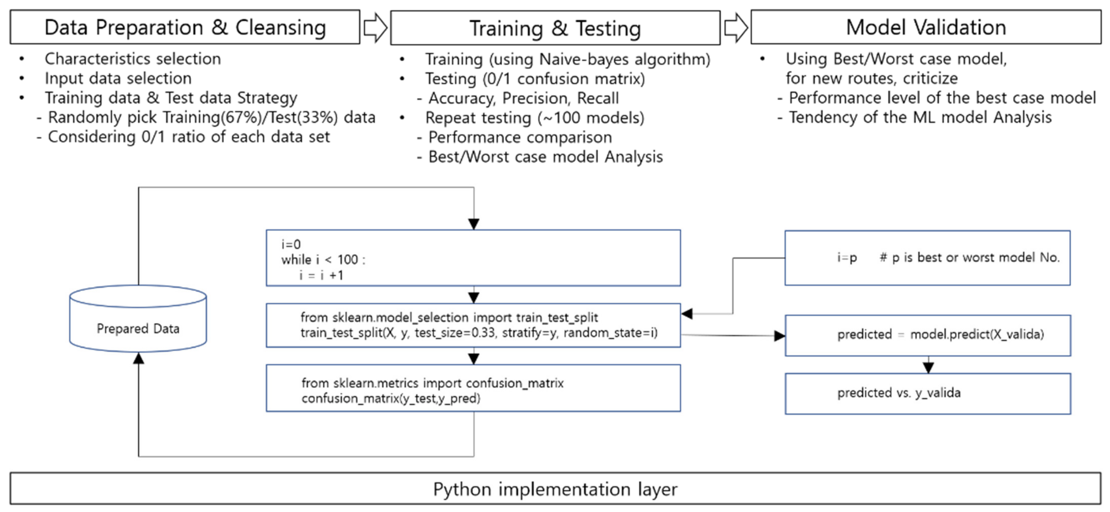
The overall flowchart of this study is shown in Figure 1. Overall, it consists of three stages. The first is a process of data preparation and cleaning, which selects characteristics for machine learning from the attributes of the secured data, and then determines that only the intact data be used as input data. The prepared data is then divided into training and testing sets. In general, the ratio of the two uses is typically 67% and 33%, allowing a 0/1 ratio for each set to be similarly divided. The reason for this, as described above, is that it affects the prediction accuracy of the machine learning model. Second, it is a way of measuring the accuracy of predictive judgment after learning with the actual Naive-Bayes algorithm, which in this study, was repeated 100 times. The best-case model and the worst-case model can be selected by comparing the performance of the 100 models. The final step is the validation step of the model. Hit accuracy is measured by determining new data that has not been used for training or testing using the corresponding prediction model, analyzing the trend of the learned model, and interpreting points to be noted for future use.
‘Scikit-learn’ is a representative machine learning library of Python [37]. This library is open source, and anyone, either individual or business, can use it for free. Scikit-learn is still under development, and it is easy to find information about it on the Internet. With it, many machine learning algorithms can be implemented for classification, regression, and clustering, and machine learning tests can be carried out immediately after installation. In this study, the ‘sklearn (a.k.a scikit-learn)’ library was used to implement a classifier using the Gaussian Naïve Bayes algorithm.
The dataset prepared for model generation and testing is the features’ values for a total of 160 routes, and the reorganization result for each route obtained from the 2020 route reorganization study. That is, for each route, it is known whether or not the decision was made to shorten or separate the corresponding route. The status of the reorganization was previously described in Table 2. Of the 160 routes, the decision was made to shorten or split for 24 routes, but not for the other 136 routes.
Python’s sklearn package provides various classes for preprocessing data, and the ‘LabelEncoder()’ function of the ‘preprocessing’ class was used to label the variables we wanted to predict, that is, a decision to shorten or not. In other words, routes where a shortened decision was made are labeled as ‘1’ (for 24 routes), and routes decided otherwise are labeled as ‘0’ (for 136 routes). When the feature data and labeled prediction data are prepared, you can import the ‘GaussianNB’ class and designate the machine learning model as ‘GaussianNB()’ to create the machine learning prediction model, that is, train it using the ‘model.fit()’ function.
The secured 160 route data were divided into a training dataset and a testing dataset. In each dataset, routes with a decision value of ‘1’ and routes with ‘0’ should be properly divided. The ‘train_test_split’ function of the ‘sklearn.model_selection’ package helps plan and execute these tasks easily.
The ‘stratify’ option is a very important option when creating a model handling classification prediction. If ‘stratify’ is specified as a classification value (prediction value) in Python code, the ratio of the class of the training dataset to the test dataset is maintained in each dataset. That is, it prevents route data with decision values of ‘1’ or ‘0’ from being concentrated and distributed in one dataset. If this ‘stratify’ option is not specified, there may be a large performance difference between the generated prediction models.
Dividing the dataset into training datasets and test datasets, and allocating routes with decisions ‘1’ and routes with ‘0’, which are important factors to consider as mentioned, can be implemented by designating the option value ‘stratify’ in the train-test-split function. In the secured dataset, 24 of the 160 routes were shortened or separated by the decision value of “1”, so the ratio of “1” is 15%. This ratio is maintained in the training dataset and testing dataset, respectively, and if you want to create an experimental set, you can set it as ‘stratify = y (forecasting variable).’
In this study, 100 experiments were conducted to create 100 predictive models. That is, 100 different learning data sets and test data sets were prepared, and the performance of each prediction model was compared. This was implemented using Python as follows. First, the ‘train_test_split’ function in the ‘sklearn.model_selection’ package was imported. This function randomly divides the 160 routes (including 24 shortened decided routes and 136 non-shortened routes) into training sets and test sets. While the relative ratio of routes with decision values of ‘1’ and routes with ‘0’ is maintained using the option ‘stratify’ as mentioned, Python randomly selects routes to generate 100 different experimental sets. In each experimental set, 67% (107 routes) of the data were set as a training data set and 33% (53 routes) were set as a testing data set. To ensure that each experiment was managed and reproducible, the ‘random_state’ argument of the ‘train_test_split’ function was utilized. The random_state argument was changed from 1 to 100, and a series of learning and testing processes were performed 100 times. This helps to repeat the model tests after learning, using the different 100 train datasets.
Each of the training and test set configuration routes of 100 different experimental sets, generated considering their randomness, are shown in Table 5. Here, route No. 65 belongs to the test set in experimental model No. 2 and the train set in experimental model No. 100. Each sets’ 0/1 ratio was maintained at 0.15, which is the ratio of the original 160 routes set.
There have been many studies on how to measure the prediction or classification performance of machine-learned classifier models [38]. Because each machine learning algorithm has its own characteristics, and indicators for measuring them differ, algorithm category, accuracy, prescription, production rate, F1-score, AUC (Area Under the Curve), etc., are generally used [39]. In this paper, the performance of the 100 generated machine learning models was compared with each other by measuring the accuracy and confusion matrix values, which are widely used to measure the performance of the Gaussian Naïve Bayes algorithm.
The accuracy of the machine learning classification or prediction model is the exact percentage of the prediction results.
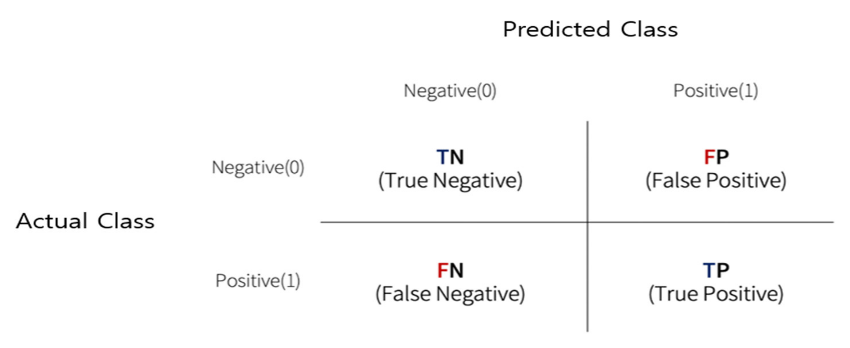
The accuracy is the most intuitive evaluation indicator of model prediction performance, but if the data imbalance is severe, other complementary performance measurement indices need to be used together. The confusion matrix indicates how confused the learned classification model is in terms of not only accuracy when predicted as a true value, but also the accuracy when predicted as a false value, so the type of prediction error can be checked. This is also called an error matrix and outputs four results which are TN, FP, FN, and TP. The definition of each result is as follows.
TN (True Negative): properly predicted actual negative data as negative.
FP (False Positive): mispredicted actual negative data as positive.
FN (False Negative): mispredicted actual positive data as negative.
TP (True Positive): real positive data is predicted positively.
After classifying the results of the machine learning models with predictors ‘0’ and ‘1’ as shown in Figure 2, several indicators representing the performance of each generated model can be evaluated to measure the predicting performance. First, ‘accuracy’ is calculated as follows.
Also, ‘precision’ and ‘recall’ can be defined as follows.
Precision is the ratio of those that are actually “1” among those that the model predicts to be “1”, which means that a model with a high value is unlikely to mistake the actual “0” situation as “1”. Meanwhile, recall is the ratio of the model prediction value predicted to be “1” among the actual “1”s, which means that the model with a high value is unlikely to mistake the actual “1” situation as “0”.
This study was conducted on Anaconda Spider (ver 4.2.5), a software execution platform in Python (ver 3.8) code and the used PC utilized an NVIDIA GeForce RTX 2080 Ti GPU on an Intel(R) Core(TM) i9-9900K CPU.
3. Numerical Results
After generating 100 models using each training and test set, the predicted values of the models were tested using the test data sets. For each model, confusion matrix results expressed as values of TN, FP, FN, and TP, were counted. The accuracy, precision, and recall indices were then calculated using them. For the machine-learned models numbered 1 to 100, the obtained test results are shown in Table 6. In each model, there were 107 routes of training data and 53 routes of test data. Accordingly, since the test prediction was made 53 times and the result was determined, the sum of TN, FP, FN, and TP for each prediction model, that is, for each row in Table 6, is 53. As a result of the obtained 100 model tests, on average, the accuracy was 72%, the precision was 22% and the recall was 36%. In the case of standard deviation, accuracy was 5.68, precision was 9.82, and recall was 18.71. On average, the fact that the recall value was higher than the precision value is interpreted to mean that this model recognizes the situation of ‘1’ well. On the other hand, it can be interpreted to mean that some of the predicted “1”s are actually mixed with “0”s.
The predicted value ‘1’ means a case where a decision to shorten or separate is required when adjusting a bus route, and ‘0’ means a case where it is not. The generated models predicted the need to shorten or separate a bus route with an average accuracy of 72%. The accuracy measurement can be seen as a probability of predicting ‘1’ for the actual ‘1’ situation and ‘0’ for the actual ‘0’ situation as described in Section 2.4. Since precision is the precision of whether the predictions of ‘1’ were actually ‘1’, the fact that the precision value turned out to be an average of 22% means that the generated machine learning models were not satisfactorily predicting the actual ‘1’ needed, and some (78%) overpredicted the need.
On the other hand, the average recall value of 36% means that the actual “1” situation was mistaken to be “0” 64% of the time with this model. This means that prediction models were somewhat sufficient in checking the need for “1” and suggested “1” for the route. To derive abundant “1” candidates, it may be a good characteristic. The trained models can be regarded as models that help experts focus on whether the routes predicted as ‘1’ are really ‘1’ rather than trying to find ‘1’s that were ‘0’.
3.1. Models and Performances
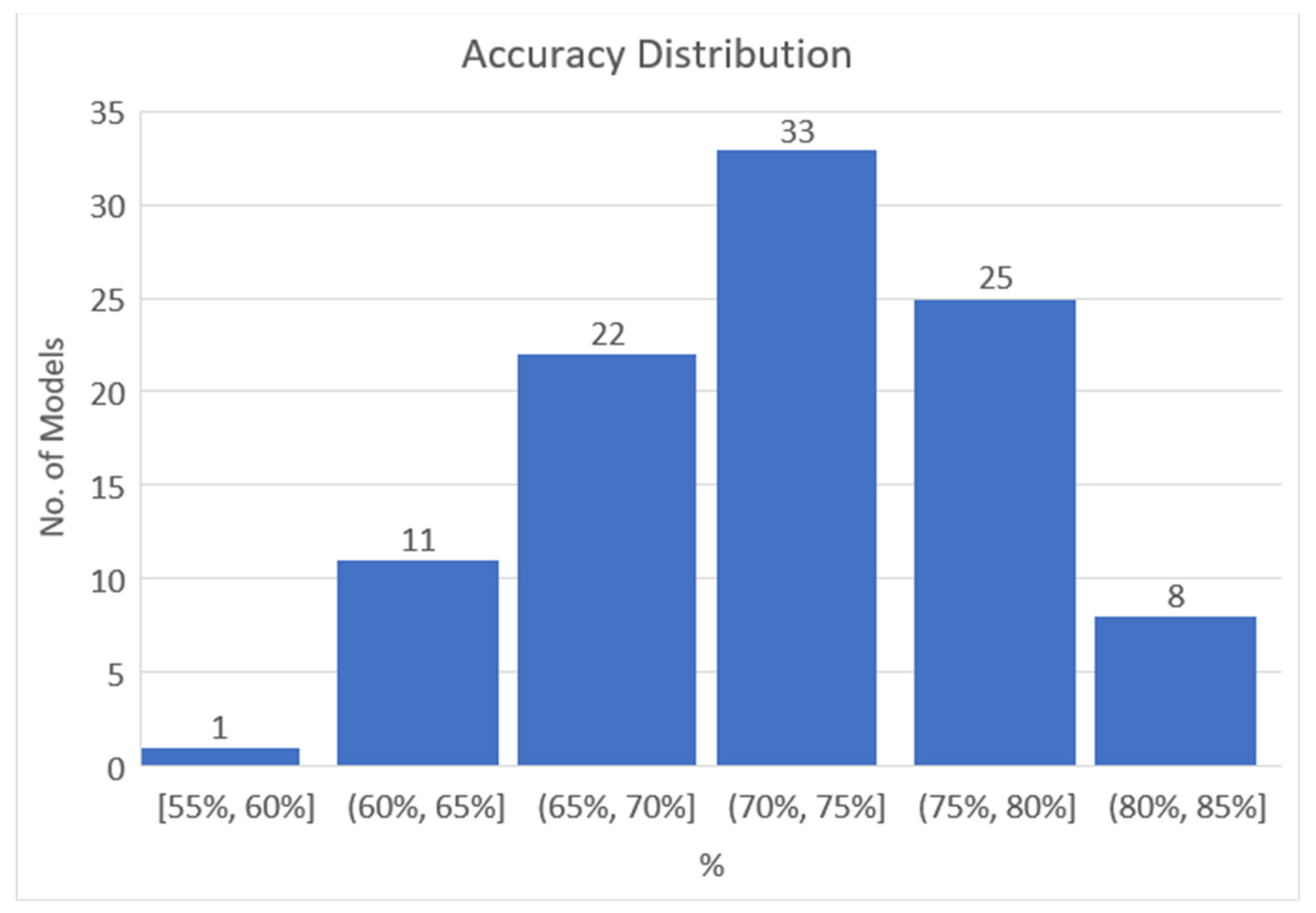
In order to examine the performance of the accuracy of the models in more detail, Figure 3 shows the distribution of the measured accuracies. As described above, the average value was 72%, the standard deviation was 5.68, the minimum value was 55%, and the maximum value was 81%. The higher the accuracy model, the higher the precision value and the recall value tended to rise together, and in the case of a model with 55% actual accuracy, the precision value was 14% and the recall value was 38%, whereas the model with 81% accuracy had 42% precision and a recall value of 63%.
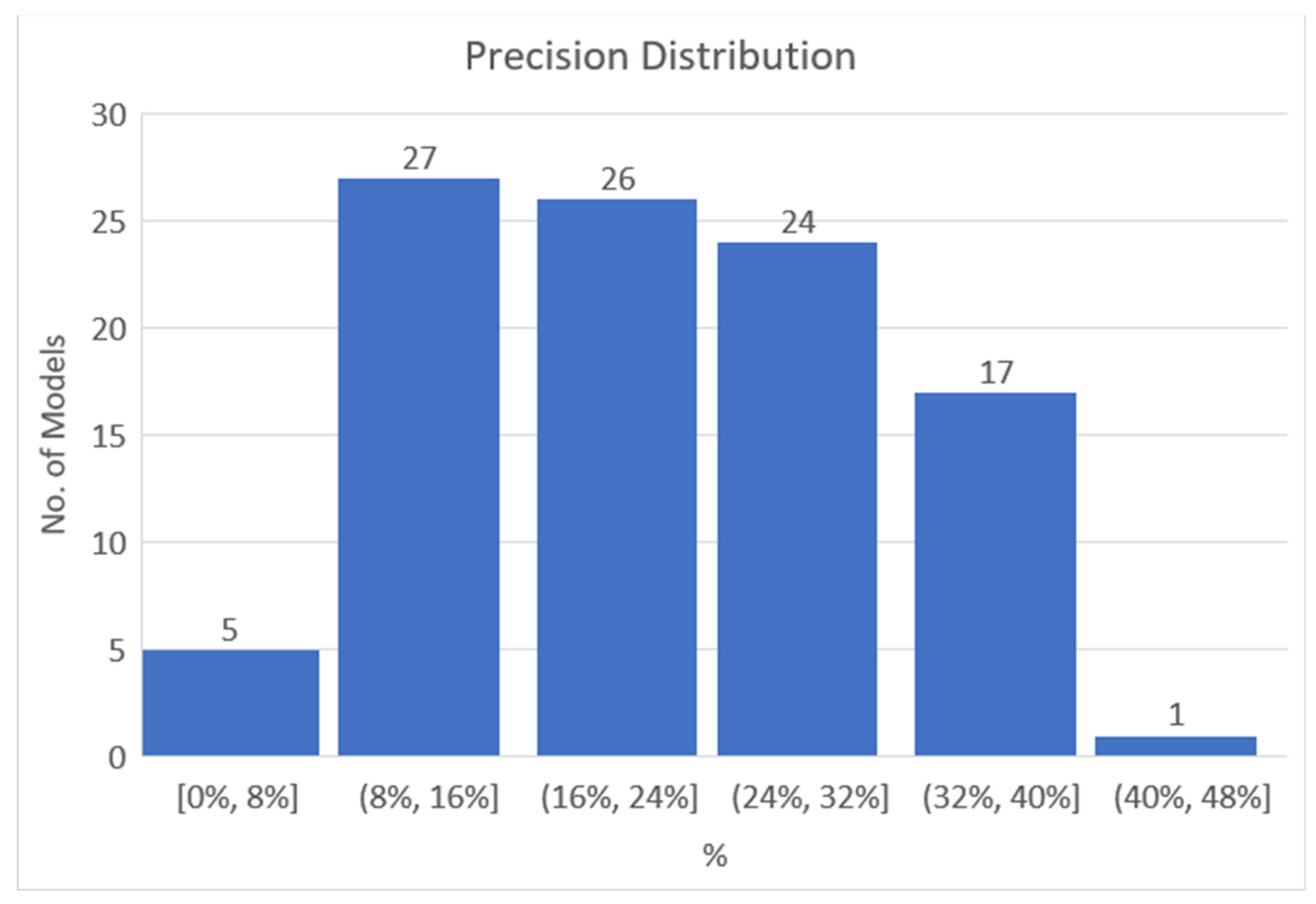
Figure 4 shows the distribution of the number of precision values of models. The average value was 22%, but the standard deviation was 9.82, with a distribution from a minimum of 0% to a maximum of 42%. The test data consisted of 53 bus routes, of which 8 routes (15%) corresponded to actual “1”. For the test set, which is a data model with a prescription value of 0%, one of the eight “1” routes was not predicted as “1”, with zero discrimination of the “1” route. Of the 100 generated models, there were the four models with 0% precision with zero discernment for ‘1’. Therefore, 4% of the generated models did not make any predictions or suggestions to be a ‘1’ route. In these four models, accuracy was 68–74%, which was only an advantage for predicting a line with ‘0’ as ‘0’.
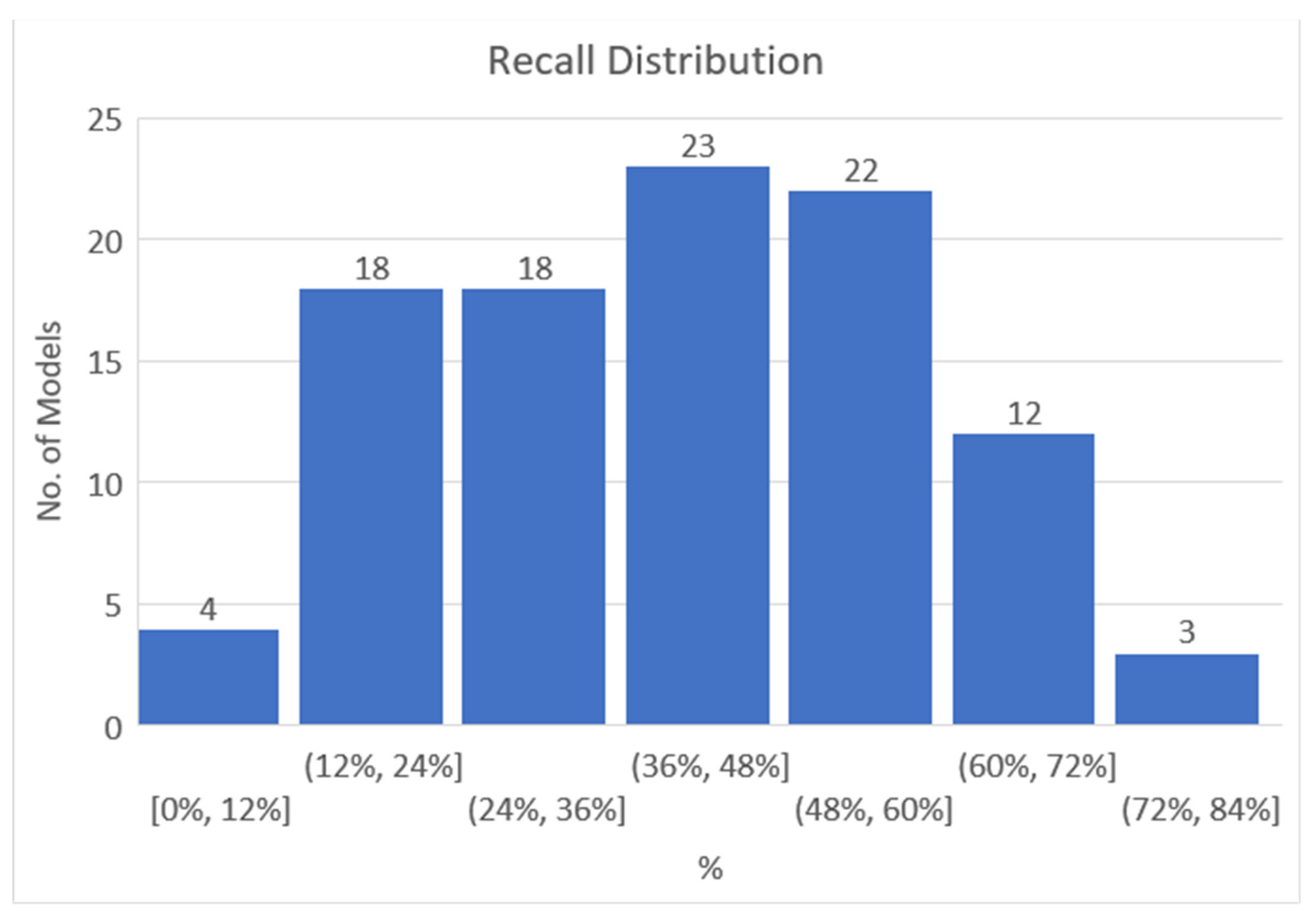
The recall values are shown in Figure 5. The average of the recall values of the 100 models was 36%, and the standard deviation was 18.71, which was somewhat large. Like the precision value, the minimum value was 0%, and the four predictive models with a recall value of 0% were models with a precision value of 0%. The maximum value was 75%, and three models were created to detect six out of eight routes corresponding to ‘1’ which existed among 53 routes in the test set.
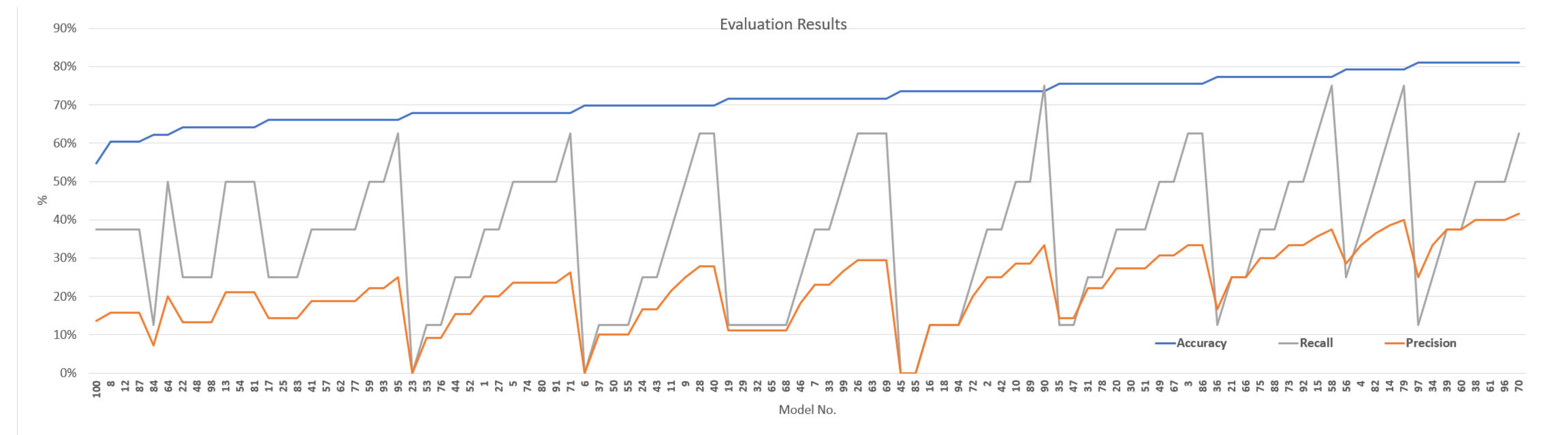
The performance values of the 100 prediction models are shown in Figure 6. As already mentioned, in general, the higher the accuracy value, the higher the recall value and the precision value. In addition, the recall index value tended to be higher than the precision value. For model #100, the model was measured with 55% accuracy, 14% precision, and 38% recall, and was the worst predictive performance model. On the other hand, model #70 showed the best predictive performance, with 81% accuracy, 42% precision, and 63% recall.
3.2. Worst and Best Models
The predictive results of the models with the worst and best accuracy are shown in Table 7. In particular, the contrasting part is the value of FP. The FP was 19 in the worst case, which indicates the number of cases where routes were predicted as ‘1’ but were actually ‘0’. This kind of confusion resulted in decreasing accuracy, in particular, in the precision value. Considering that the predictive model we present here causes performance degradation by recommending ‘1’ a lot, routes predicted as “1” can be seen as cases that require a closer review. On the other hand, in the best case, the number of FP was good at 7, which resulted in 81% accuracy and 42% precision value.
The characteristics of the 19 routes confused with FP in the worst model are examined. Table 8 lists the “0” routes with their characteristics, that is, 19 FP routes that the model mistook for ‘1’ among 53 test data routes for the worst-case model. Additionally, for the best model results, FP mistakes are also shown in the table, together with that of the worst model. Among the bus routes shown in the table, No. 532 is the only branch line, and the rest are all trunk lines. Fortunately, this means that the machine-learned model was well embedded in the main decision-making attribute, regardless of the worst and best models, which is the basic attribute of a route requiring shortening or separation.
Although not always, it is generally true that trunk lines are subject to priority consideration when it comes to shortening or separation, and trunk lines are longer in length and have longer operating times than branch lines. Three bus routes showed FP results, both in the worst model and in the best model, and those routes were ‘2-1’, ‘66’, and ‘72’. These routes were classified into long-distance routes that had one-time operating times of more than three hours, 200 min, 238 min, and 258 min, respectively. These three routes can be identified as routes that should be shortened or recommended separately. The three routes were the most common candidates indeed. The reorganization study report showed that these three routes were actually determined to be “0” because of their role in replacing closed routes and the only route connecting beyond the city boundary to local airports, and so on.
In addition, the route reorganization results, which are the basic data in this study, were compared with the results recommended by the best model. Specifically, the results were compared with the overall route prediction results recommended by model 70, as shown in Table 9. According to this study, the performance of the best predictive model had 94% accuracy, 70% precision, and 88% recall based on the entire data of the route reorganization case.
3.3. Virtual Experiment
Virtual experiments to verify the effectiveness of the developed model could be easily conducted if there is an opportunity to apply the machine-learned prediction model to bus route reorganization research in other cities. Alternatively, if additional bus route reorganization research case data for other cities can be secured, it will be possible to verify the model’s recommendation or prediction ability compared to the final reorganization results. The developed data model could be used as the first classifier for shortening recommendable routes. However, it is not easy to secure data on other cities, so this study briefly verifies the effectiveness of the model with the secured data.
Case study data obtained for this study included data on a total of 199 routes, as shown in Table 2. From the perspective of data completeness, only data from 160 routes, excluding 39 routes, were used for the data modeling research. Of the 39 routes excluded, we were able to reuse a total of 14 routes through additional data surveys and the application of estimation formulas for some missing fields. The data on the 14 routes obtained through this process could have been used as developed model input. Information on the 14 routes to be used for the virtual experiment is shown in Table 10. This table shows the predictions to which the worst model was applied and the predictions to which the best model was applied, respectively.
As shown in the table, among the total 14 virtual experimental routes two routes were determined to be “maintained” and 12 routes were determined to be “suspension.” These decisions are values other than shortening or separation decisions, so the actual values are ‘0’. The results of predictive classification for these 14 routes with the worst and best models are shown in Table 10. The worst model showed 57% accuracy, and the best model showed 85% accuracy. However, what is remarkable about this virtual experiment is that there were only routes with an actual value of “0”, so it was not possible to confirm how each prediction model predicted the actual situation of “1”. Nevertheless, what has been clearly verified is that the worst model overestimated the ‘1’ candidate route compared to the best model.
It was necessary to examine the route review history for route No. 909 and route No. 598, which were shortened or separately recommended by the best model. No. 909 was replaced by another route with a similar route, but it was interpreted that the recommendation for shortening was appropriate because the operating time exceeded 190 min. On the other hand, for No. 598 a follow-up survey showed that the effect of separation was observed because two new routes 208 and 223 were efficiently backed up instead of being suspended. Therefore, the model prediction value for No. 598 may be interpreted as an appropriate ‘1’ recommendation result.
4. Conclusions
This study discusses whether machine-learned city bus route improvement recommenders can perform well enough to help make decisions. In fact, by using data from preliminary research on route reorganization, the study of machine learning models was expected to be able to generate an effective prediction model. The modeling and test results showed an average prediction accuracy of 72%. The Naïve Bayes algorithm, a machine learning model, which was selected for reasons such as lack of learning data, characteristics of predictors, and similarities with existing applications, was efficiently implemented through Python’s ‘sklearn’ package and helped test 100 repetitive model generation tasks considering randomness.
We could validate the machine learning model generated through predictive opinions on bus routes that were not related to the data used for training and testing. And although these should be considered limited conditions, we were able to verify that it showed 57–85% predictive accuracy. The limited condition here is that there was no data with an actual value of ‘1’ in the model verification data set, which is expected to be re-verified through additional data acquisition.
The purpose of the route improvement prediction classifier developed in this study was basically to determine how accurately and abundantly the route to be shortened or separated could be recommended to route improvement experts and related researchers. When reviewing the models developed from that point of view, the worst model with the lowest accuracy and recall value tended to classify the predicted (recommended) values as ‘1’ for routes that were not finally selected to be shortened or separated. In the case of the best model, with high accuracy and recall value, routes that could be shortened were recommended at a level similar to the actual decision-making results, and routes with a high recall value of ‘1’ were detected at the level of 63%. Model verification was conducted using virtual experiments. By verifying the attributes of the shortened recommended routes using actual circumstances, we were able to confirm that the model prediction was appropriate by comparing the contents of the route improvement study with the recommendation by model prediction.
160 bus route data were used in this study, including for learning and testing. Although the use of the Naive-Bayes algorithm demonstrated its potential for developing a classifier capable of machine learning with a small amount of data, the methodology proposed in this study could be further improved with more modeling and accuracy. Securing additional datasets could also be helpful to further validate the model. In addition, since there were false cases, where the probabilistic independence between characteristic variables assumed by the Naive-Bayes algorithm was incorrect, the algorithm could be further refined by supplementing it with a model that introduces weights for each characteristic variable.
For the reorganization of bus routes, the machine learning model, which recommends an improved direction for each route, can be expanded and developed in the following ways in the future.
- Application and evaluation of various machine learning classification algorithms
- Proposed methodology for multiple classifications (deciding extension of route, detour, etc.) rather than 0/1 classification
- Development and Research of Data Models for Pre-learning of Transfer Learning Concepts
In addition to research on how to improve bus routes with the existing optimization concept, it is expected that various bus route optimization studies using machine learning will be published in the future.
Consequently, it was verified that the route shortening possibility prediction and route classification recommender presented in this study could be useful for recommending route improvements through data-based machine-learned artificial intelligence. Based on the case data of bus route reorganization in Incheon City, the newly developed predictive model is expected to be further refined using additional data from other cities and additional model learning and testing processes.
Author Contributions
Writing—original draft preparation, M.-h.S.; writing—review and editing, M.J. All authors have read and agreed to the published version of the manuscript.
Funding
This research was supported by Ministry of Science and ICT, Republic of Korea (Project No. K-22-L02-C04-S01).
Acknowledgments
We would like to express appreciation to Incheon Metropolitan City, Korea, for the research data used in this study.
Conflicts of Interest
The authors declare no conflict of interest.
References
- Belokurov, V.; Spodarev, R.; Belokurov, S. Determining passenger traffic as important factor in urban public transport system. Transp. Res. Procedia 2020, 50, 52–58. [Google Scholar] [CrossRef]
- Dulebenets, M.A. An Adaptive Island Evolutionary Algorithm for the berth scheduling problem. Memetic Comput. 2020, 12, 51–72. [Google Scholar] [CrossRef]
- Albayrak, M.B.K.; Ozcan, I.C.; Can, R.; Dobruszkes, F. The determinants of air passenger traffic at Turkish airports. J. Air Transp. Manag. 2020, 86, 101818. [Google Scholar] [CrossRef]
- Abioye, O.F.; Dulebenets, M.A.; Kavoosi, M.; Pasha, J.; Theophilus, O. Vessel schedule recovery in liner shipping: Modeling alternative recovery options. IEEE Trans. Intell. Transp. Syst. 2021, 22, 6420–6434. [Google Scholar] [CrossRef]
- Enoch, M.P.; Cross, R.; Potter, N.; Davidson, C.; Taylor, S.; Brown, R.; Huang, H.; Parsons, J.; Tucker, S.; Wynne, E.; et al. Future local passenger transport system scenarios and implications for policy and practice. Transp. Policy 2020, 90, 52–67. [Google Scholar] [CrossRef]
- Ceder, A. Public Transit Planning and Operation: Modeling, Practice and Behavior; CRC Press: Boca Raton, FL, USA, 2016. [Google Scholar]
- Yajima, M.; Sakamoto, K.; Kubota, H. Efficacy of bus service reorganization utilizing a hub-and-spoke topology and DRT to meet community needs: A case study of Tokigawa town. IATSS Res. 2013, 37, 49–60. [Google Scholar] [CrossRef] [Green Version]
- Hatzenbühler, J.; Cats, O.; Jenelius, E. Network design for line-based autonomous bus services. Transportation 2021, 49, 467–502. [Google Scholar] [CrossRef]
- Ren, H.; Wang, Z.; Chen, Y. Optimal Express Bus Routes Design with Limited-Stop Services for Long-Distance Commuters. Sustainability 2020, 12, 1669. [Google Scholar] [CrossRef] [Green Version]
- Chien, S.I.; Dimitrijevic, B.; Spasovic, L.N. Optimization of Bus Route Planning in Urban Commuter Networks. J. Public Transp. 2003, 6, 53–79. [Google Scholar] [CrossRef] [Green Version]
- Chuah, S.P.; Wu, H.; Lu, Y.; Yu, L.; Bressan, S. Bus Routes Design and Optimization via Taxi Data Analytics. In Proceedings of the 25th ACM International on Conference on Information and Knowledge Management, CIKM ′16, Indianapolis, IN, USA, 24–28 October 2016; pp. 2417–2420. [Google Scholar] [CrossRef]
- Kim, K.S.; Dickey, J. Role of urban governance in the process of bus system reform in Seoul. Habitat Int. 2006, 30, 1035–1046. [Google Scholar] [CrossRef]
- Ceder, A.; Wilson, N.H.M. Bus Network Design. Transp. Res. Part B Methodol. 1986, 20, 331–344. [Google Scholar] [CrossRef]
- Lampkin, W.; Saalmans, P.D. The Design of Routes, Service Frequencies, and Schedules for a Municipal Bus Undertaking: A Case Study. J. Oper. Res. Soc. 1967, 18, 375–397. [Google Scholar] [CrossRef]
- Van Oudheusden, D.L.; Ranjithan, S.; Singh, K.N. The Design of Bus Route Systems—An Interactive Location-Allocation Approach. Transportation 1987, 14, 253–270. [Google Scholar] [CrossRef]
- Pattnaik, S.B.; Mohan, S.; Tom, V.M. Urban Bus Transit Route Network Design Using Genetic Algorithm. J. Transp. Eng. 1998, 124, 368–375. [Google Scholar] [CrossRef]
- Szeto, W.Y.; Wu, Y. A Simultaneous Bus Route Design and Frequency Setting Problem for Tin Shui Wai, Hong Kong. Eur. J. Oper. Res. 2011, 209, 141–155. [Google Scholar] [CrossRef] [Green Version]
- Lin, J.-J.; Wong, H.-I. Optimization of a Feeder-Bus Route Design by Using a Multiobjective Programming Approach. Transp. Plan. Technol. 2014, 37, 430–449. [Google Scholar] [CrossRef]
- Ahern, Z.; Paz, A.; Corry, P. Approximate Multi-Objective Optimization for Integrated Bus Route Design and Service Frequency Setting. Transp. Res. Part B Methodol. 2022, 155, 1–25. [Google Scholar] [CrossRef]
- Benn, H.P. Bus Route Evaluation Standards; Transportation Research Board: Washington, DC, USA, 1995; ISBN 0309058554. [Google Scholar]
- Vakulenko, K.; Kuhtin, K.; Afanasieva, I.; Galkin, A. Designing Optimal Public Bus Route Networks in a Suburban Area. Transp. Res. Procedia 2019, 39, 554–564. [Google Scholar] [CrossRef]
- Papola, A.; Tinessa, F.; Marzano, V.; Mautone, A. Quantitative Overview of Efficiency and Effectiveness of Public Transport in Italy: The Importance of Using ITS. In Proceedings of the 2017 5th IEEE International Conference on Models and Technologies for Intelligent Transportation Systems (MT-ITS), Naples, Italy, 26–28 June 2017; pp. 895–900. [Google Scholar] [CrossRef]
- Liu, W.; Teng, J.; Zhang, D. Performance Evaluation at Bus Route Level: Considering Carbon Emissions. In Proceedings of the ICTE 2013—Proceedings of the 4th International Conference on Transportation Engineering, Ottawa, ON, Canada, 11–12 June 2013. [Google Scholar]
- Jiménez, F.; Román, A. Urban Bus Fleet-to-Route Assignment for Pollutant Emissions Minimization. Transp. Res. Part E Logist. Transp. Rev. 2016, 85, 120–131. [Google Scholar] [CrossRef]
- Simonelli, F.; Tinessa, F.; Marzano, V.; Papola, A.; Romano, A. Laboratory Experiments to Assess the Reliability of Traffic Assignment Map. In Proceedings of the 2019 6th International Conference on Models and Technologies for Intelligent Transportation Systems (MT-ITS), Cracow, Poland, 5–7 June 2019; pp. 1–9. [Google Scholar] [CrossRef]
- Jordan, M.I.; Mitchell, T.M. Machine learning: Trends, perspectives, and prospects. Science 2015, 349, 255–260. [Google Scholar] [CrossRef]
- Kotsiantis, S.B. Supervised machine learning: A review of classification techniques. In Proceedings of the 2007 Conference on Emerging Artificial Intelligence Applications in Computer Engineering: Real Word AI Systems with Applications in eHealth, HCI, Information Retrieval and Pervasive Technologies, Online, 10 June 2007; Volume 160, pp. 3–24. [Google Scholar]
- Mohamed, A.E. Comparative Study of Four Supervised Machine Learning Techniques for Classification. Int. J. Appl. Sci. Technol. 2017, 7, 5–18. [Google Scholar]
- Kotsiantis, S.B.; Zaharakis, I.D.; Pintelas, P.E. Machine learning: A review of classification and combining techniques. Artif. Intell. Rev. 2006, 26, 159–190. [Google Scholar] [CrossRef]
- Soofi, A.A.; Awan, A. Classification Techniques in Machine Learning: Applications and Issues. J. Basic Appl. Sci. 2017, 13, 459–465. [Google Scholar] [CrossRef]
- Cunningham, P.; Cord, M.; Delany, S.J. Supervised Learning. In Machine Learning Techniques for Multimedia. Cognitive Technologies; Cord, M., Cunningham, P., Eds.; Springer: Berlin/Heidelberg, Germany, 2008. [Google Scholar] [CrossRef]
- Park, D. Image Classification Using Naïve Bayes Classifier. Int. J. Comput. Sci. Electron. Eng. 2016, 4, 135–139. [Google Scholar]
- Rish, I. An empirical study of the naive Bayes classifier. In Proceedings of the IJCAI 2001 workshop on empirical methods in artificial intelligence, Seattle, WA, USA, 4–6 August 2001; Volume 3. [Google Scholar]
- Sethi, J.K.; Mittal, M. Efficient weighted naive bayes classifiers to predict air quality index. Earth Sci. Inform. 2022, 15, 541–552. [Google Scholar] [CrossRef]
- Nadinta, D.S.; Surjandari, I.; Laoh, E. A Clustering-Based Approach for Reorganizing Bus Route on Bus Rapid Transit System. In Proceedings of the 2019 16th International Conference on Service Systems and Service Management (ICSSSM), Shenzhen, China, 13–15 July 2019; pp. 1–6. [Google Scholar]
- Jahromi, A.H.; Mohammad, T. A non-parametric mixture of Gaussian naive Bayes classifiers based on local independent features. In Proceedings of the 2017 Artificial Intelligence and Signal Processing Conference (AISP), Shiraz, Iran, 25–27 October 2017. [Google Scholar]
- Available online: https://scikit-learn.org/ (accessed on 1 January 2022).
- Available online: https://developers.google.com/machine-learning/crash-course (accessed on 1 January 2022).
- Wardhani, N.W.S.; Rochayani, M.Y.; Iriany, A.; Sulistyono, A.D.; Lestantyo, P. Cross-validation Metrics for Evaluating Classification Performance on Imbalanced Data. In Proceedings of the 2019 International Conference on Computer, Control, Informatics and Its Applications (IC3INA), Tangerang, Indonesia, 23–24 October 2019. [Google Scholar] [CrossRef]
Figure 1.
A schematic diagram of the whole process flow.

Figure 2.
Meanings of four results of the confusion matrix.

Figure 3.
Accuracy distribution of the classifier models.

Figure 4.
Precision distribution of the classifier models.

Figure 5.
Recall distribution of the classifier models.

Figure 6.
Performance of 100 models.


Table 1.
Summary of literature for bus route reorganization.
| Category | Model and Method Characteristics | Ref. No. |
|---|---|---|
| Bus Route Design &Optimization | Two-stage Stochastic Programming | [13] |
| Global optimization using decoupling with heuristic | [14] | |
| Set covering algorithm (at fixed demand), Simple Plant Location Problem | [15] | |
| Genetic Algorithm for simultaneous decision of route length and no. of routes | [16] | |
| Multi-objective Function of transit and travel timeGenetic Algorithm with heuristic | [17] | |
| Multi-objective Optimization under UncertaintyConsidering multiple stakeholders | [18] | |
| Multi-objective Function of passenger and bus operationSimulated Annealing | [19] | |
| Bus Route Evaluation &Scenario Planning | Bus route evaluation standard | [20] |
| Scenario-based Planning for suburban areas, KPI Estimation | [21] | |
| Performance evaluation of transportation system, KPI Estimation | [22] | |
| Considering Carbon Emission usingAssignment Model | Carbon Emission model for a bus system | [23] |
| Carbon Emission model for bus routes | [24] | |
| Transportation Assignment Model | [25] |
Table 2.
Route change decisions made in the case reorganization study.
| Decisions | Counts | Detailed Data Incomplete | Detailed Data Complete |
|---|---|---|---|
| Shortened | 21 | - | 21 |
| Separated | 3 | - | 3 |
| Changing path | 38 | 2 | 36 |
| Extended | 16 | - | 16 |
| Merged | 8 | - | 8 |
| Maintained | 89 | 22 | 67 |
| Suspension | 24 | 15 | 9 |
| Total no. of routes | 199 | 39 | 160 |
Table 3.
Sample of the secured data for the case reorganization study.
| Type | Bus No. | Enterprise Name | Enterprise Address | Starting Bus Stop | Ending Bus Stop | First Round Time | Last Round Time |
|---|---|---|---|---|---|---|---|
| Trunk | 205 | YP | West | Youngjong | Airport | 4:50 | 22:55 |
| Seat | 790 | SK | West | Suhyun | Youngheu | 4:15 | 20:40 |
| Trunk | 700-1 | KHSJ | KH | KH | Terminal | 5:20 | 22:00 |
| … | … | ||||||
| Length (km) | No. of Vehicles | One round time (min) | No. of rounds | Interval time_min (min) | Interval time_max (min) | Transfer trips per round | |
| 61.3 | 6 | 120 | 54 | 18 | 20 | 26 | |
| 118.86 | 6 | 275 | 21 | 45 | 55 | 1771 | |
| 154.3 | 10 | 396 | 25 | 36 | 43 | 3425 | |
| … | … | … | … | … | … | … | |
| First ride trips per round | Velocity (km/h) | Average PHT (min) | Average PKT (km) | Passengersper round | |||
| 330 | 35.7 | 18.44 | 11.34 | 356 | |||
| 5326 | 27.13 | 47.31 | 26.04 | 7097 | |||
| 10,484 | 25.79 | 26.84 | 10.74 | 13,909 | |||
| … | … | … | … | … | |||
Table 4.
10 features of routes to be input to the model.
| Features | Name | Variable Type |
|---|---|---|
| 1 | Length (km) | Floating point |
| 2 | No. of Vehicles | Integer |
| 3 | One round time (min) | Integer |
| 4 | No. of rounds | Integer |
| 5 | Interval time_min (min) | Integer |
| 6 | Interval time_max (min) | Integer |
| 7 | Velocity (km/h) | Floating point |
| 8 | Passengers per round | Integer |
| 9 | Transfer trips per round | Integer |
| 10 | First ride trips per round | Integer |
Table 5.
Comparison of 100 generated model input routes.
| Model # | Train Data Set Route # (107 Routes) | Test Data Set Route # (53 Routes) | ||||||||||||
|---|---|---|---|---|---|---|---|---|---|---|---|---|---|---|
| 1 | 203 | 566 | 584 | … | 512 | 700-1 | 31(c) | 535 | 43-1 | 591-1 | … | 569 | 591 | 300 |
| 2 | 35 | 308 | 103 | … | 800 | 593 | 17-1 | 304 | 571 | 43 | … | 564 | 65 | 303 |
| 3 | 223 | 202 | 72 | … | 42 | 79 | 592 | 13 | 515-1 | 4 | … | 535 | 117 | 24 |
| … | … | … | … | … | … | … | … | … | … | … | … | … | … | … |
| 100 | 558 | 20 | 700-1 | … | 82 | 65 | 60-5 | 2-1 | 790 | 521 | … | 585 | 80 | 63 |
Table 6.
Test results for runs #1~#100 of the machine-learned prediction model.
| Model # | # of TN | # of FP | # of FN | # of TP | Accuracy (%) | Precision (%) | Recall (%) |
|---|---|---|---|---|---|---|---|
| 1 | 33 | 12 | 5 | 3 | 68 | 20 | 38 |
| 2 | 36 | 9 | 5 | 3 | 74 | 25 | 38 |
| 3 | 35 | 10 | 3 | 5 | 7 + 5 | 33 | 63 |
| … | … | ||||||
| 100 | 26 | 19 | 5 | 3 | 55 | 14 | 38 |
| Average (%) | 72 | 22 | 36 | ||||
| δ(std. dev.) (%) | 5.68 | 9.82 | 18.71 | ||||
Table 7.
Test results of the worst and best models.
| Case | Model # | # of TN | # of FP | # of FN | # of TP | Accuracy (%) | Precision (%) | Recall (%) |
|---|---|---|---|---|---|---|---|---|
| Worst | 100 | 26 | 19 | 5 | 3 | 55 | 14 | 38 |
| Best | 70 | 38 | 7 | 3 | 5 | 81 | 42 | 63 |
Table 8.
19 FP routes of the prediction results for model #100 (Worst model) and model #70 (Best model).
Table 8.
19 FP routes of the prediction results for model #100 (Worst model) and model #70 (Best model).
| Bus No. | Whether Worst Model FP or Not | Whether Best Model FP or Not |
|---|---|---|
| 532 | O | - |
| 112 | O | - |
| 13 | O | - |
| 79 | O | - |
| 800 | O | - |
| 4 | O | - |
| 14-1 | O | - |
| 22 | O | - |
| 6-1 | O | - |
| 14 | O | - |
| 78 | O | - |
| 303 | O | - |
| 10 | O | - |
| 38 | O | - |
| 65-1 | O | - |
| 63 | O | - |
| 2-1 | O | O |
| 66 | O | O |
| 72 | O | O |
| 5 | - | O |
| 1 | - | O |
| 70 | - | O |
| 42 | - | O |
Table 9.
Best case model results for the actual route reorganization data.
| Case | Model # | # of TN | # of FP | # of FN | # of TP | Accuracy (%) | Precision (%) | Recall (%) |
|---|---|---|---|---|---|---|---|---|
| Best | 70 | 129 | 7 | 3 | 21 | 94 | 70 | 88 |
Table 10.
14 routes’ information for the virtual experiment.
| Bus No. | Decision of the Case Study | Actual Value of Case Study | Predictions by the Worst Model | Predictions by the Best Model |
|---|---|---|---|---|
| 701 | Maintained | 0 | 0 | 0 |
| 702 | Maintained | 0 | 0 | 0 |
| 721 | Suspension | 0 | 1 | 0 |
| 754 | Suspension | 0 | 1 | 0 |
| 760 | Suspension | 0 | 0 | 0 |
| 760-1 | Suspension | 0 | 0 | 0 |
| 770-1 | Suspension | 0 | 0 | 0 |
| 780-2 | Suspension | 0 | 0 | 0 |
| 904-1 | Suspension | 0 | 1 | 0 |
| 905 | Suspension | 0 | 0 | 0 |
| 908 | Suspension | 0 | 1 | 0 |
| 909 | Suspension | 0 | 1 | 1 |
| 598 | Suspension | 0 | 1 | 1 |
| 598-1 | Suspension | 0 | 0 | 0 |
| Accuracy (%) | 57 | 85 | ||
Publisher’s Note: MDPI stays neutral with regard to jurisdictional claims in published maps and institutional affiliations. |
© 2022 by the authors. Licensee MDPI, Basel, Switzerland. This article is an open access article distributed under the terms and conditions of the Creative Commons Attribution (CC BY) license (https://creativecommons.org/licenses/by/4.0/).
Share and Cite
MDPI and ACS Style
Suh, M.-h.; Jeong, M. Development of Bus Routes Reorganization Support Software Using the Naïve Bayes Classification Method. Sustainability 2022, 14, 4400. https://0-doi-org.brum.beds.ac.uk/10.3390/su14084400
AMA Style
Suh M-h, Jeong M. Development of Bus Routes Reorganization Support Software Using the Naïve Bayes Classification Method. Sustainability. 2022; 14(8):4400. https://0-doi-org.brum.beds.ac.uk/10.3390/su14084400
Chicago/Turabian StyleSuh, Min-ho, and Minjoong Jeong. 2022. "Development of Bus Routes Reorganization Support Software Using the Naïve Bayes Classification Method" Sustainability 14, no. 8: 4400. https://0-doi-org.brum.beds.ac.uk/10.3390/su14084400
Note that from the first issue of 2016, this journal uses article numbers instead of page numbers. See further details here.