
Estimation of the Urban Heat Island Effect in a Reformed Urban District: A Scenario-Based Study in Hong Kong


1
Department of Land Surveying and Geo-Informatics, The Hong Kong Polytechnic University, Hung Hom, Hong Kong, China
2
Research Institute for Land and Space, The Hong Kong Polytechnic University, Hung Hom, Hong Kong, China
*
Author to whom correspondence should be addressed.
Sustainability 2022, 14(8), 4409; https://0-doi-org.brum.beds.ac.uk/10.3390/su14084409
Submission received: 4 March 2022
/
Revised: 23 March 2022
/
Accepted: 30 March 2022
/
Published: 7 April 2022
(This article belongs to the Special Issue Sustainability Challenges in Urban Heat Island Mitigation Strategies)
Abstract
:Urban heat island (UHI), a phenomenon in which land surface temperatures (LSTs) in an urban area are notably higher than that in the surrounding rural area, has made the living environment thermally uncomfortable, endangered public health, and increased the energy consumption on indoor air cooling. To develop a liveable and sustainable city, it is crucial to provide an accurate estimation of the UHI effect for urban planners when an area is transformed from bare lands to a high density of buildings. With this objective, the study develops multivariate spatial regression models based on LSTs retrieved from Landsat-8 thermal images to estimate the distribution of urban heat magnitudes (i.e., UHMs, relative temperatures referenced to rural temperature), by considering four types of causative factors that include land use and land cover, urban morphology, heat source, and local climate zones. Partial correlation analysis is performed to determine explainable variables and R2 is used to evaluate the models. Based on the constructed models and a master plan of buildings in Kowloon East, Hong Kong, the future UHM distributions are forecasted on four representative days in different seasons. Results show that the UHI effect will be mitigated significantly when the new buildings are built, suggesting appropriate urban planning regarding the urban thermal environment. We found that the considered factors can largely explain the daytime UHIs in both the built-up areas and land-cover areas. The proposed method can also be used to optimize the urban design for creating a more thermo-friendly urban environment.
1. Introduction
The urban heat island (UHI), a phenomenon that air temperatures or land surface temperatures (LSTs) are generally higher in urban areas than its surrounding rural areas, is a significant anthropogenic alteration to the Earth’s environment [1]. The acceleration of global urbanization exacerbates the UHI effect, resulting in a variety of consequences, such as atmospheric environment intervention [2], regional climate change [3], enhanced vegetation growth [4,5], and air and water pollution by disrupting the surface-energy balance [6]. Meanwhile, UHI can increase energy consumption [7], endanger human health [8], and considerably obstruct the development of environmentally sustainable cities [9].
In response to these issues, an early study assessed the UHI effect by considering multiple influential factors, such as canyon radiative geometry, thermal characteristics of buildings and vegetation, anthropogenic heat emission, and turbulent transmission [10]. According to one study, natural terrain (e.g., soil, vegetation, and water bodies) was gradually being replaced by impervious artificial surfaces (e.g., asphalt, and concrete) that reduced evapotranspiration and increased the sensitive heat, which was especially noticeable in high-density areas [11]. Another study found that rapid building construction, as well as the emergence and spread of skyscrapers, exacerbated the UHI effect [12].
The above studies imply that the spatial configuration of buildings and the thermal environment are the root causes of UHI. On this basis, numerous indicators have been proposed to perform correlation analysis with the urban heat magnitude (UHM) defined by the temperature difference between urban and rural areas, which can be classified into three causative categories: (i) land use and land cover (LULC) that can be described by normalized difference vegetation index (NDVI) [13], normalized differential build-up index (NDBI) [14], and tree cover ratio and shrub cover ratio [15], (ii) urban morphology (UM) that can be depicted by floor area ratio and building density [15], sky view factor (SVF) [16], and building surface fraction and fabric density ratio [17], and (iii) thermal and radiative property (TRP) that can be represented by solar irradiation [18], surface albedo [17], and wind velocity [19,20].
It is discovered that these indicators have varying effects on UHMs. For example, UHMs are increasing in proportion to the amount of thermal mass absorbed by cities [20,21,22,23]. While the UHI effect will be mitigated when the vegetation cover ratio is high because vegetation increases latent heat transfer in the air via transpiration and evaporation [4,5,24,25], and UHMs are decreasing in areas where there are more high rises buildings casting significant shadows [20,23,26,27]. However, these studies did not account for the regional effects of the urban landscape, which can create a variety of microclimates and thus have a significant impact on the urban thermal environment.
Since it has been demonstrated that the UHMs can be largely explained by background climate in over 30,000 global cities [28] and urban form in 1288 Chinese urban clusters [29], it is reasonable to develop a model that integrates microclimate with the above three causative categories for a better understanding of the UHI effect. This is critical for climatic modelling and may even be useful for urban planning and weather forecasting [2], which is a growing concern for urban planners [30]. Therefore, there is a trend to deepen from tracking spatio-temporal dynamic behaviour of UHIs [31,32] and gaining an in-depth understanding of the UHI formulation [28,29] to propose solutions to mitigate the UHI phenomenon, such as optimizing locations of green space [33].
The new trend necessitates the development of a robust model capable of evaluating and even mitigating the UHI effect through urban design, which has not been well established yet. To address this issue, this study aims to: (i) propose and determine UHI related indicators by considering comprehensive effects from microclimates and the three categorized indicators, (ii) investigate spatial and seasonal variations of UHMs in a densely urban area and build spatial regression models to estimate seasonal changes of UHMs, and (iii) predict UHM distribution in different seasons based on a master plan of buildings.
2. Literature Review
2.1. Local Climate Zones
Regarding urban microclimate, one novel study developed a categorization system to classify urban areas into 17 different local climate zones (LCZs), particularly for the study of UHIs [34]. There are two types of LCZs: (i) ten built type LCZs (i.e., LCZ-1 to LCZ-10) that are composed of artificial structures on a prevailing land cover, which are either compact zones with paved surfaces or open zones covered by low plants or scattered trees, and (ii) seven land cover type LCZs (i.e., LCZ-A to LCZ-G) that describe dominant land covers. For instance, LCZ-1 denotes a compact highrise landscape, whereas LCZ-A denotes dense trees. Because LCZs provide descriptive information essentially, they can be used as classifiers to perform correlation analysis for each LCZ or category variable in mathematical modelling. Thus, the UHMs can be estimated using the four categorized factors of LCZ, LULC, UM, and TRP, which requires a set of spatio-temporal associated datasets and a robust regression model.
2.2. Land Surface Temperatures
To estimate UHMs accurately, all datasets should be organized in the same spatio-temporal domain, where UHMs can be represented by air temperatures or LSTs. Although air temperatures can be recorded at the high-temporal resolution, they typically lack large coverage at the high-spatial resolution due to the scarcity of monitoring stations [35], which contradicts this study that requires a detailed investigation of the UHI effect over a large urban area. Alternatively, LSTs retrieved from satellite thermal images can be used to quantify UHMs because they can provide spatially continuous observations of the temperatures in urban areas [36,37]. This is critical for enabling spatial association with UHM-related indicators, even though the temporal resolution is lower.
2.3. Regression Models
To assess the effects of urban planning indicators, Lin et al., (2017) conducted linear regressions between the UHMs and land use indicators (i.e., floor area ratio, building density, and park area) and greenery indicators (i.e., tree cover ratio) [15], respectively. It is found that the floor area ratio, building density, and tree cover ratio had a strong and negative correlation with the UHMs during the daytime, and the park area was cooler than the surrounding urban streets during both daytime and nighttime. Using a similar multi-linear regression, it was found that the UHI effect increased with the logarithm of the urban size but decreased with the logarithm of the anisometry based on the 5000 European cities [38]. In another study, quadratic equations were created between LST and each individual indicator (e.g., NDVI, NDBI, and digital elevation model) in four study areas, which achieved high correlations for some indicators [39]. According to the study, green and blue space ratios, road networks, and housing distributions all had a significant impact on UHIs.
Furthermore, spatial regression models were developed to build regressions between LSTs and six indicators, including impervious surface area proportion, vegetation area proportion, water proportion, SVF, building density, and floor area ratio [40]. With the consideration of spatial autocorrelation, it was demonstrated that the spatial error model (SEM) with a spatially correlated error term was outperformed the spatial lag model (SLM) with a spatially correlated dependent term in the study area, based on R2, loglikelihood, AIC, and Schwarz criteria. A similar study combined SEM and SLM to build the regressions between LSTs and the influential indicators (i.e., building ground floor area, water, solar irradiation, NDVI, and SVF), suggesting the effectiveness of the model to mitigate UHIs through urban design [18]. The two studies imply that spatial regression models are effective, which will also be developed in our study to investigate the UHI effect. Rather than focusing on the absolute LST [18,40], this study will use HUM, a relative temperature subject to the referenced rural temperature, as the dependent variable of the model, which can represent the UHI effect more accurately. Unlike the previous study [38] comparing the UHI effects in multiple urban areas, this study will comprehensively investigate the seasonal effects of LCZ, LULC, UM, and TRP on UHIs in a densely urban area.
Multi-linear regression models were developed to predict UHI intensity based on key parameters (i.e., SVF, surface albedo, vegetation density ratio, and building surface fraction) classified by LCZs [17]. Few studies have been conducted to optimize urban planning to reduce the UHI effect. One study proposed weighted multi-objective modelling to predict the cooling effect during both daytime and nighttime by optimizing locations of green space [33]. The objective function was solved repeatedly by varying the weights between 0 and 1, identifying the most significant benefits based on the day-versus-night cooling trade-offs. In comparison, this study is significant since it will incorporate all four types of causative factors (LCZ, LULC, UM, and TRP) into the spatial regression modelling to quantify the UHI and a comprehensive framework will be developed to predict the future thermal environment based on a planned urban landscape rather than optimizing the cooling effect.
This study is innovative in three major aspects. First, the UHI influential factors are proposed and modelled systematically with the consideration of heat sources, urban microclimates, urban morphology, and land use and land cover. Second, the spatio-temporal effects of the influential factors are quantified and evaluated by developing multivariate regression models for the four seasons. Third, the UHI distribution in a reformed urban area is predicted across different seasons based on a master plan of buildings, which is important for guiding urban planning on creating a comfortable urban thermal environment.
3. Estimation of the UHI and UHS
3.1. Definitions of the Urban Heat Magnitude
Urban heat island (UHI) and urban heat sink (UHS) have been widely defined as urban areas where their temperatures (e.g., land surface temperatures) are higher or lower than the referenced rural temperature, respectively [41,42]. To investigate the effects of urban climates on the UHI and UHS phenomena, the concept of Local Climate Zone (LCZ) is used, which proposes a standard method for characterizing and classifying holistic urban landscapes with the consideration of micro-scale land-cover and physical properties [34]. The study suggested that each LCZ presents a distinct urban landscape defined by specific geometry and surface cover attributes [34], making it an appropriate candidate for UHI and UHS research. LCZs are categorized into 17 zones, which contain ten built types from LCZ-1 to LCZ-10 to describe densely populated zones with varying building densities, heights, and distances, and seven land-cover types from LCZ-A to LCZ-G to denote different natural environments. With the consideration of LCZs in this study, the average LST in LCZ-D (i.e., low plants) is used as the referenced rural temperature, and a UHI and a UHS are defined as a local climate zone where its LSTs are higher or lower than the referenced LST. Based on this definition, urban heat magnitude (UHM) is proposed as the LST difference (Equation (1)) between the LCZ-X and LCZ-D, where LCZ-X represents any one of the ten built types (LCZ-1 to LCZ-10) or seven land cover types (LCZ-A to LCZ-G).
∆T = LSTX − LSTD
3.2. Research Framework for Building the UHM Estimation Model
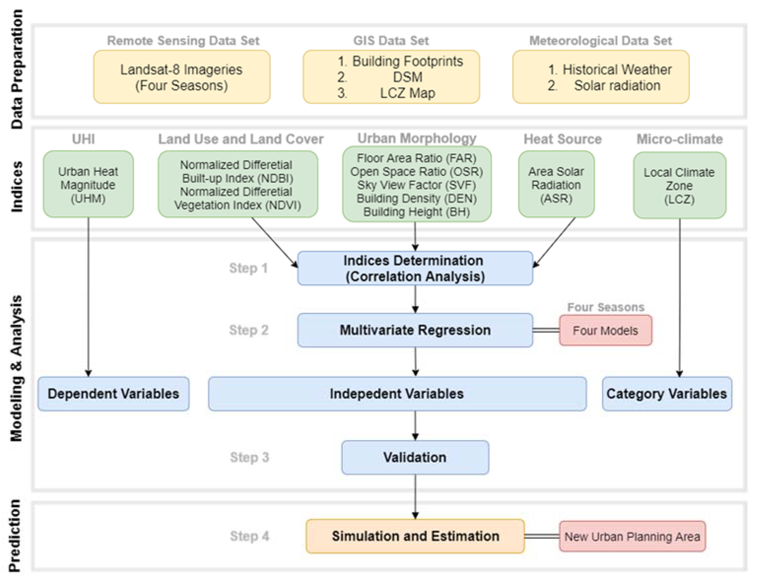
This study proposes a model to estimate UHMs in a planned urban area as shown in Figure 1, which is composed of four major steps. First, the model is based on a series of datasets, including the remote sensing dataset (i.e., Landsat-8 imagery), GIS dataset (i.e., building footprints, DSM, and the map of LCZs), and meteorological dataset (i.e., historical weather, and solar irradiation). Second, a set of spatial indicators are proposed that can be categorized into the dependent variable (i.e., UHMs), independent variables (i.e., eight indices to represent UM, LULC, and TRP), and category variable (i.e., LCZs). Third, spatial correlations between the proposed indicators and the UHMs can be built and analyzed to determine the indicators that can be used to explain the UHI and the UHS effect. On this basis, for each season, a spatially multivariate regression model is built based on the determined explicable indicators. Fourth, based on the established spatial regression models, the UHMs can be predicted based on a determined master plan of the buildings.
3.3. Multivaritate Regression
This study assumes that heat source (i.e., solar irradiation accumulated during the daytime), land use and land cover (e.g., represented by normalized difference vegetation index), urban morphology (e.g., represented by sky view factor), and local climate zones affect UHMs comprehensively. When the UHM influential factors are determined based on the correlation analysis, multivariate regression can be built to quantify the effects of these indicators on UHMs on a specific day. Particularly, when incorporating LCZs to describe a diverse landscape, the LCZ classification will be used as a category matrix in the regression, which is supposed to improve the estimation accuracy of UHMs, compared with a uniform model without the distinction of LCZs. This is because different LCZs are likely influencing the UHMs heterogeneously, which is also suggested by previous studies [34,43,44,45].
Since all the types of LCZs are quite complex and could not be considered simply as built-up areas or land cover areas, LCZs are incorporated into the regression as category variables to obtain accurate mathematic modelling. To build a multivariate regression model, a set of spatial contiguous and homogenous grid cells are created firstly at an appropriate spatial resolution to cover the whole study area, and then the proposed indices are calculated for each grid cell, resulting in the same number of the samples for all the indicators that can be used to build multivariate regressions. In the model, there are two steps to select effective indicators. One is correlation analysis to determine the explainable indicators, and the other is a regression coefficient test aiming to get the significant indicators. The tolerance (O) and variance inflation factor (VIF) will be calculated to ensure the indicators are not multicollinear before building a multivariate regression model following Equation (2), where Y is the dependent variable, C1 and C2 are a vector of regression coefficients, X1 is the matrix of UHM related variables, X2 is the matrix of LCZ category variables, and ε is a vector of random errors.
Y = C1 × 1 + C2 × 2 + ε
3.4. Retrieval of Land Surface Temperature
The LST can be calculated in a variety of ways [46,47]. This study converts top of atmosphere brightness temperature to calculate LSTs based on band 10 of the Landsat-8 satellite’s Thermal Infrared Sensors [48]. The Digital Numbers (DN) from the raw Landsat-8 images are converted to Top of Atmosphere (TOA) reflectance values based on Equation (3):
where Lλ is the TOA spectral radiance in the unit of Watts/(m2 × srad × μM), ML and AL are the band-specific multiplicative rescaling factor and the band-specific additive rescaling factor obtained from the metadata, respectively, and Qcal is the quantized and calibrated standard product DNs. Then, using the thermal constants included in the metadata file of the Landsat-8 product, thermal bands can be converted from spectral radiance to TOA brightness temperature in Equation (4), where T is the TOA brightness temperature (K), and K1 and K2 are the band-specific thermal conversion constants from the metadata.
Lλ = MLQcal + AL
3.5. Modelling of the UHM Indicators
3.5.1. Normalized Differential Built-Up Index (NDBI)
NDBI is a spectral index to execute a legitimate and realistic relationship between LST and the built-up area in a city [23,49]. NDBI ranges between [−1, 1] that negative values represent vegetation, while positive values represent built-up areas. NDBI can be calculated using Landsat OLI data in Equation (5), in which SWIR is the short-wave infrared band (band 6 for Landsat-8), and NIR is the near-infrared band (band 5 for Landsat-8).
3.5.2. Normalized Difference Vegetation Index (NDVI)
NDVI is the widely used and most popular index for vegetation assessment, which ranges between [−1, 1] [25,50]. The negative values present areas predominated by clouds, water, and snow, around-zero values suggest areas primarily occupied by rocks and barren soil, moderate values (from 0.2 to 0.3) represent shrubs and meadows, and large values (from 0.6 to 0.8) represent temperate and tropical forests. NDVI can be calculated in Equation (6) by using the red and near-infrared (NIR) bands [51], where NIR is the near-infrared band (i.e., band 5 for Landsat-8) and R is the red band (i.e., band 4 for Landsat-8).
3.5.3. Sky View Factor (SVF)
SVF is the ratio between the radiation received in the plane and the radiation environment of the entire hemisphere [52], which is an important index combining building height and building density. The spatial distribution of SVF is closely related to the urban morphologies impacting the urban thermal environment [53]. SVF ranges from 0 to 1, and a larger value indicates a broader-view sky. The SVF is calculated from a particular place while considering all nearby obstructions to the sky hemisphere [54]. SVF can be calculated based on Equation (7):
3.5.4. Area Solar Radiation (ASR)
Solar irradiation varies significantly over spatio-temporal domains in a city [55], which is considered to be an important heat source of UHIs that occur during the daytime. To take this effect into consideration, the accumulation of solar irradiation is simulated by using the Areal Solar Radiation toolset in ArcGIS Pro [56] which models the effects from urban morphology and atmospheric conditions quantified by transmittivity (t) and diffuse proportion (d). Specifically, t was calculated in Equation (8) by using the proportion of the specific days that were clear, partly cloudy, and cloudy (Pclear, Ppartlycloud, and Pcloudy), assuming the three weights are 0.70, 0.50, and 0.30, and d is calculated based on Equation (9) that the three corresponding weights are 0.20, 0.45, and 0.70 [57].
t = 0.70Pclear + 0.50Ppartlycloud + 0.30Pcloudy
d = 0.20Pclear + 0.45Ppartlycloud + 0.70Pcloudy
3.5.5. Building Indicators
In addition, four building indicators are proposed to delineate the urban morphology, including building height (BH), building density (DEN), open space area (OSR), and floor area ratio (FAR), which are essential indicators in urban planning. In particular, BH is a measure of a region’s average building height (Equation (10)), DEN is the percentage of all building footprints in a district (Equation (11)), OSR is the amount of outdoor open space relative to the total floor area (Equation (12)), and FAR measures the total volume of regional buildings (Equation (13)). In the equations, n represents the number of buildings, Hi is the height of a building, Ai represents the base area of the buildings in a grid cell, and Al is the area of a grid cell.
4. Empirical Investigation
4.1. Study Area
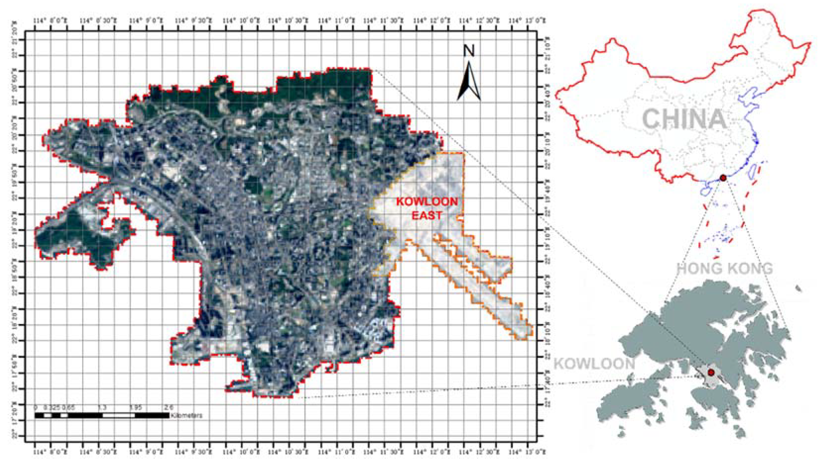
The Kowloon district in Hong Kong has a population of over 2.24 million people [58] in an area of about 46.95 km2 [59], making it one of the world’s most densely populated areas. Since the Hong Kong Government has established an initiative to convert the east part of Kowloon (i.e., Kowloon East covering an area of 3.74 km2, as shown in Figure 2) from bare land to a commercial and business district [60], it is critical for urban planners to make this region thermally comfortable, considering that the UHI effect is a significant phenomenon in Hong Kong that has made several adverse impacts to the society [61,62]. As a result, it is appropriate for this study to construct a UHM prediction model based on the observation of the Kowloon district and evaluate the UHI effect in the planned urban area of Kowloon East.
4.2. Data Collection
This study collected a series of datasets adaptive to the proposed model. To observe seasonal UHI effects under the same atmospheric condition, this study selects four sunny days in four different seasons with few cloud-cover, based on the weather records obtained from the Hong Kong Observatory [63]. The four days are on 1 April 2018 (in spring), 20 August 2017 (in summer), 14 November 2019 (in autumn), and 2 December 2020 (in winter), all of which had stable weather without the influence of strong wind and typhoon during the past 24 h. Since cloud cover can determine transmittivity and diffuse proportion conclusively and hence influence solar irradiation significantly, historical cloud cover data for the corresponding days is obtained from World Weather Online [64]. Then, Landsat-8 satellite images captured at 10:58 am are downloaded from the United States Geological Survey [65] to compute LSTs.
To build a UHM estimation model considering the effects of urban morphology, building footprints (17,296 buildings in total) enriched with the height attribute in the entire Kowloon area are obtained from the Lands Department of the Hong Kong Government. To predict UHMs of the constructed Kowloon East area, the master plan of buildings in Kowloon East, including the building blocks and the height attributes, is also obtained from the Station Planning Portal 2 [66]. In addition, The Lands Department provided the Digital Surface Model (DSM) covering the whole Kowloon area so that the SVF can be calculated at a resolution of 10 m. Since different local climate zones may affect UHM differently, the LCZ dataset [67] is obtained for investigating UHMs in the group of LCZs. According to the dataset metadata, the overall LCZ classification accuracy in Hong Kong is 0.749 and the built-up area accuracy is 0.941. The model is built with an integration of the spatial database management system (DBMS) and ArcGIS Pro.
4.3. Data Pre-Processing
4.3.1. Mapping of the LCZs and SVFs
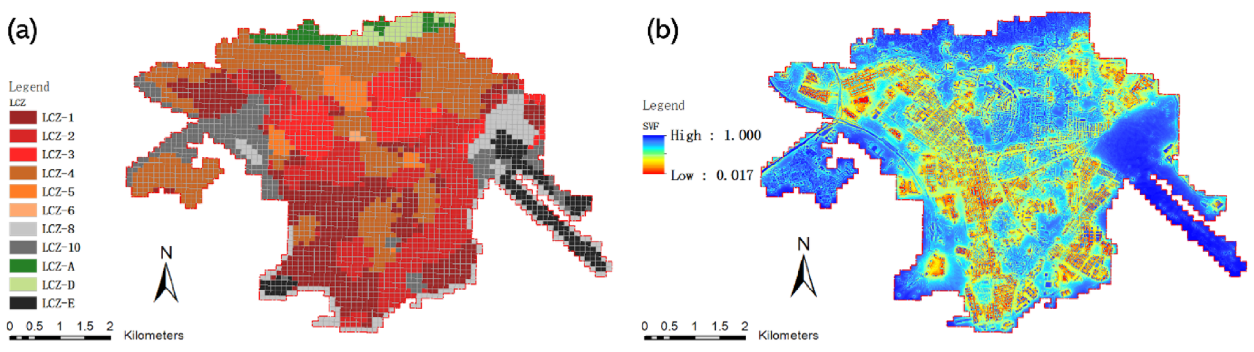
There are 3048 grid cells (i.e., 3048 data samples) in Kowloon when the statistical grid cells are at 100 m resolution. Eleven types of LCZs are identified in the Kowloon area, with built-up types (LCZs 1-6, 8, and 10) counting for 2772 grid cells (91% of the area) and land-cover types (LCZs A, D, and E) counting for 276 grid cells (9% of the area), as shown in Figure 3a and Table 1. The mean LST for LCZ-D in central urbanized Kowloon was chosen as the referenced rural temperature to calculate UHMs as it represents vegetation in urban areas. Also, SVFs are computed and presented in Figure 3b. Based on this, the average UHM in each grid cell is obtained by calculating the LST difference between LCZ-D (i.e., low plants) and the others.
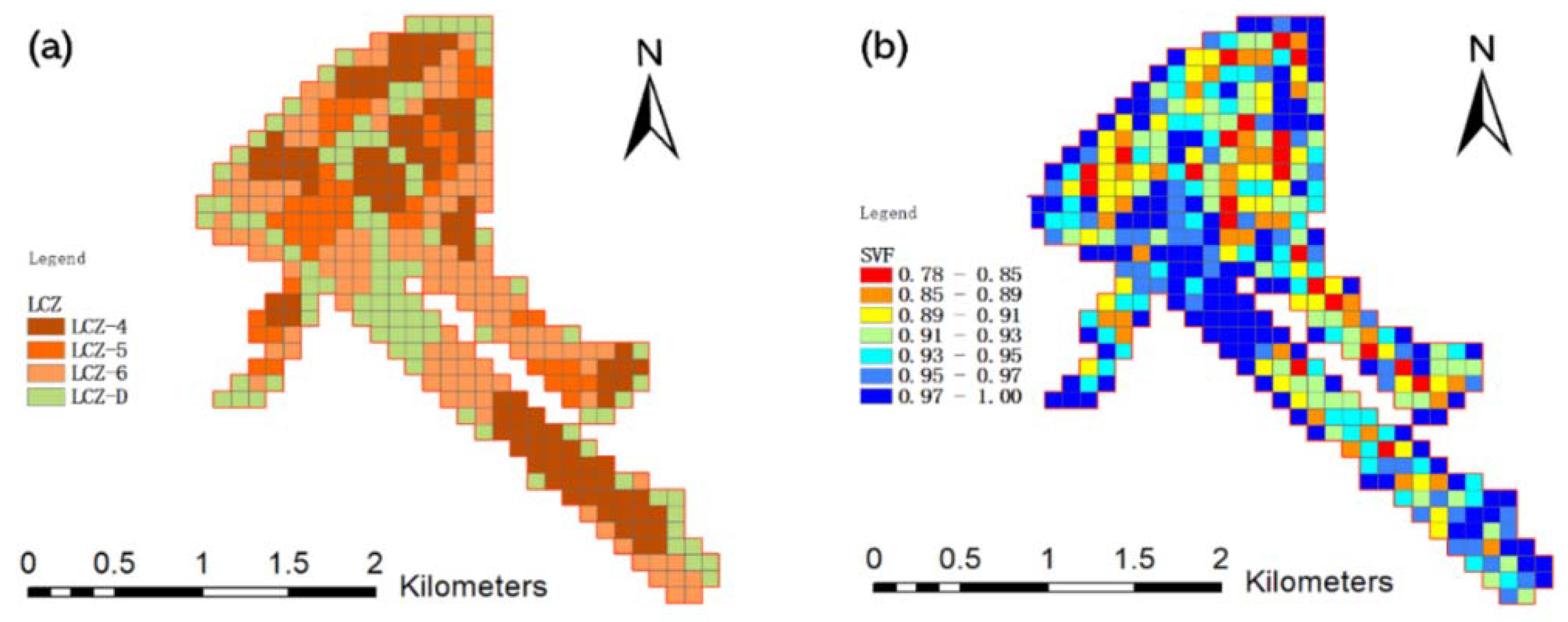
The planned urban area of Kowloon East is about 3.2 km2, which will provide about 2 million square meters of building area for residences, offices, and hotels [68]. Based on the LCZ classification rules, there will be four LCZs in the Kowloon East area as shown in Figure 4a, including 27.27% LCZ-4, 13.64% LCZ-5, 33.15% LCZ-6 in built-up types, and 25.94% LCZ-D in land-cover types (Table 2). Meanwhile, the future SVFs are presented in Figure 4b. Thus, 374 grid cells with 100 m resolution are generated so that all the indicators are spatially associated in the DBMS. Based on this, UHMs in the planned area can be estimated when spatial regression models are built.
4.3.2. Mapping of UHMs in Kowloon
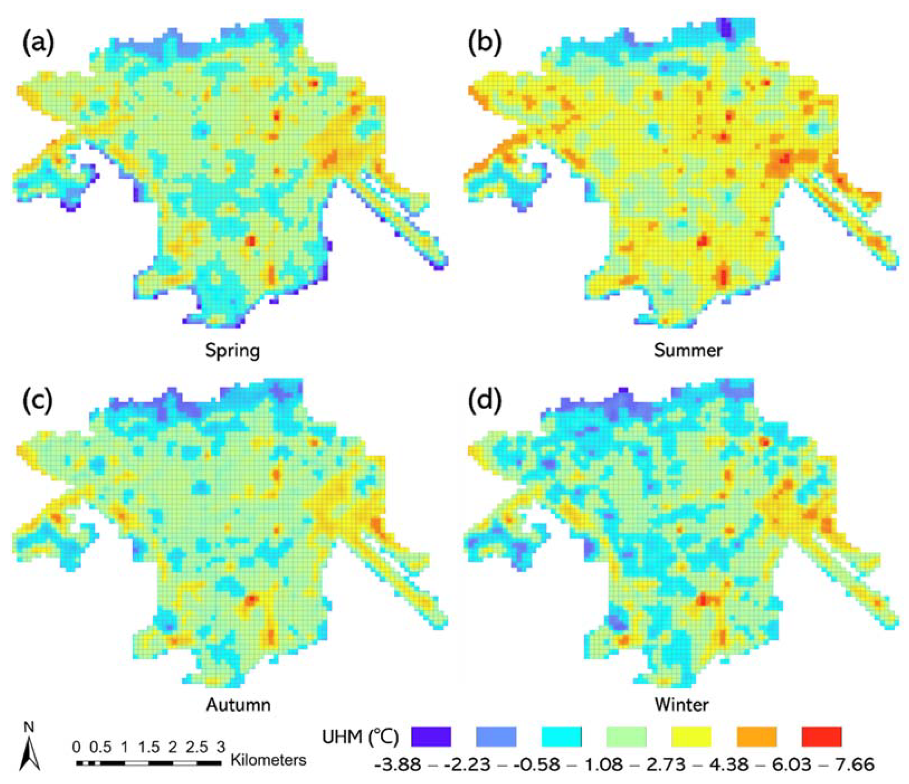
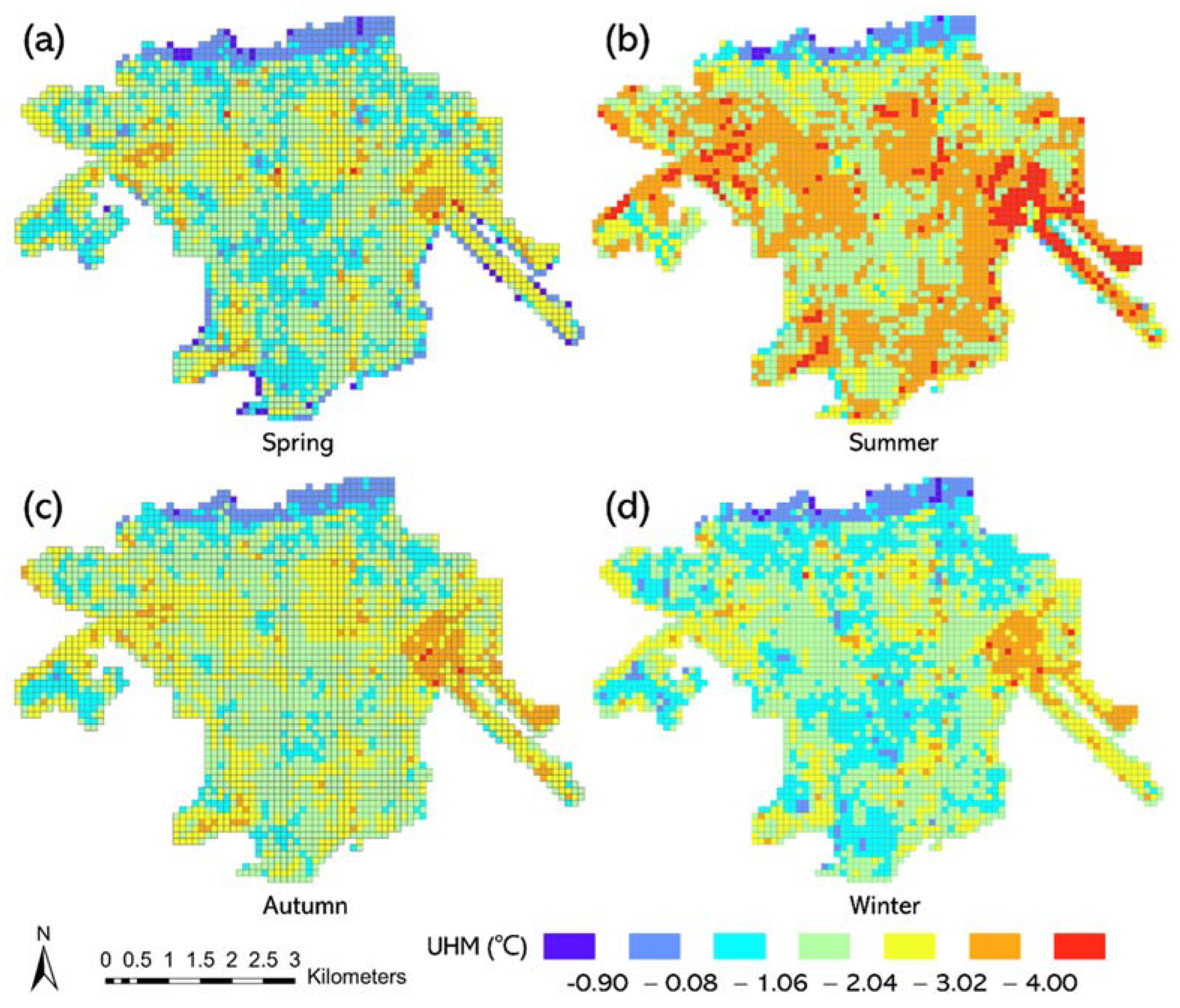
Figure 5 presents the spatial distribution of UHMs in Kowloon on four representative days to indicate four different seasons, which shows that Kowloon has a heterogeneous distribution of UHMs and the maximum UHM is at 7.66 °C. It also clearly demonstrates that high UHMs are mainly located in Kowloon East that is being transformed from bare land to built-up areas and in Hung Hom with a large area of concrete surfaces, while low UHMs are concentrated in city parks (e.g., the Kowloon Park) and mountain forest (e.g., Lion Rock Country Park). In spring and autumn, the spatial distribution of UHMs is quite similar to each other. In comparison, UHMs exhibit apparent distinctions in summer and winter that UHMs range between 2.73 °C and 4.38 °C in summer, while UHMs are between 0 °C and 1.08 °C in winter. This suggests that the daytime UHI effect is the most significant in summer in Hong Kong than in the other three seasons. There can be two reasons. First, the study area can accumulate a large amount of heat from solar irradiation quickly during the daytime in summer, which increases the impervious land surface temperature significantly. Second, buildings and vehicles use air conditioners extensively that generate and release more heat into the air in summer, which exacerbates the UHI effect.
4.3.3. Mapping of Area Solar Irradiation
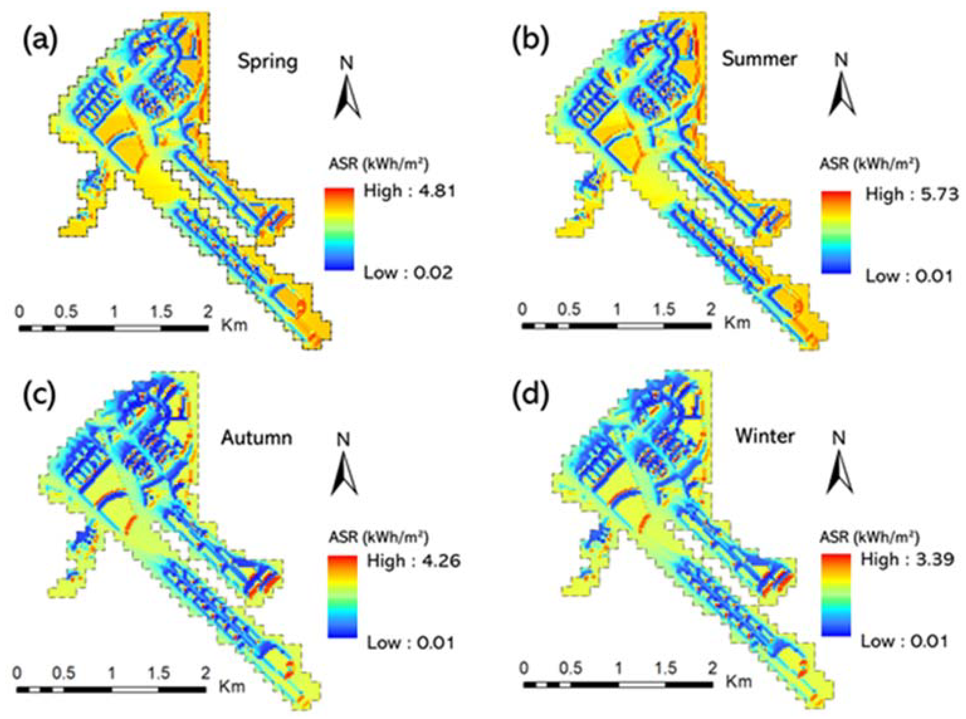
Based on the cloud cover statistics, transmissivity and diffuse proportion are computed to estimate the spatial distribution of solar irradiation accurately (Table 3), and the four seasons are classified as spring from March to May, summer from June to August, autumn from September to November, and winter from December to the following February. The large transmittivities and small diffuse proportions imply that the four days were cloud-free, therefore solar irradiation could be one of the most important heat sources of the investigated UHIs. It is because LSTs were computed based on Landsat-8 thermal images that were acquired at nearly 11 am in the local time. Based on the corresponding atmospheric condition, solar irradiation on the planned urban surfaces can also be accumulated from early morning to the time instant when the satellite image is acquired on the four days (Figure 6), which will be used to predict the UHMs when the multivariate regression model is established.
5. Results
5.1. Identification of the Influential Indicators
It is supposed that the proposed eight indicators can affect UHMs in four seasons with varying significance. To determine the correlation between the indicators and the UHMs across the 3048 grid cells in the study area, multivariate regressions are made on each of the four days independently and the statistics are presented in Table 4, where R is Pearson’s correlation coefficient, PR denotes Partial R, and p is significant level. It is important to notice that this study has also computed the tolerance (O) and the variance inflation factor (VIF) to examine the multicollinearity. It is found that there is no apparent collinearity between the indicators because O is larger than 0.1 and VIF is smaller than 10 [69,70]. Since BH (i.e., building height) and OSR (i.e., open space ratio) have significances (p) larger than 0.05 on all four days, BH and OSR will not be considered as the influential factors to the UHM, leading to the determination of the remaining six indicators that affect UHIs.
5.2. Distribution of the Indicators across LCZs
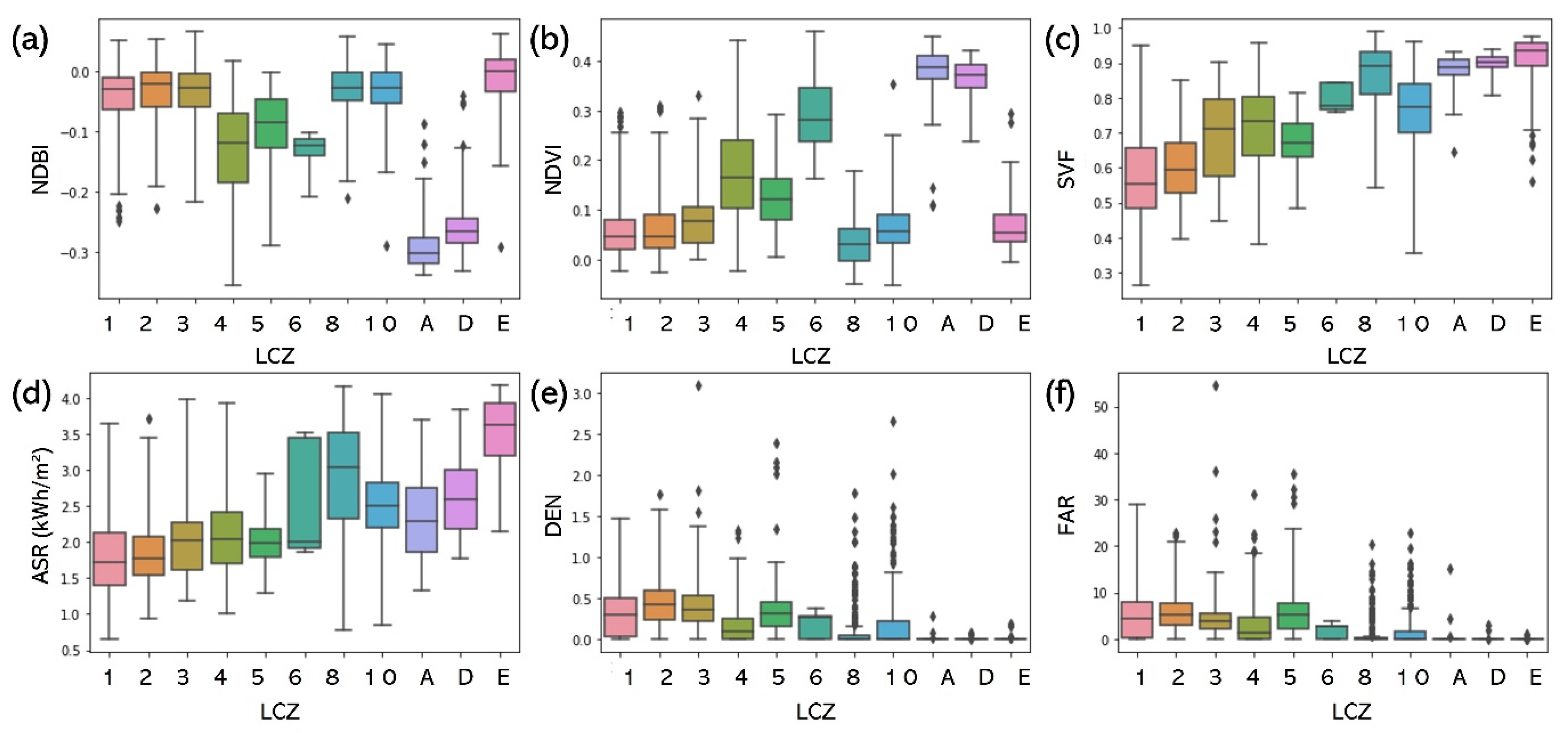
Figure 7 depicts the distribution of the proposed indicators (in the y-axis) across eleven types of the LCZs (in the x-axis) on 20 August 2017. Figure 7a,b show that NDBI and NDVI exhibit an inverse distribution. Specifically, NDVI increases from compact highrise (LCZ-1) to open lowrise (LCZ-6), with a relatively low distribution in open midrise (LCZ-5), similar to NDBI. Note that the distribution of NDBI and NDVI in LCZ-E is distinct from the other land cover types because it is located in the bared rock and paved surface. In comparison, SVF shows an upward trend for LCZs from the left to the right side of the x-axis in Figure 7c. In detail, SVF has a wide range between 0.25 and 0.95, and the 50th percentiles increase stably from LCZ-1 to LCZ-4, which corresponds to the built-up area changing from compact highrise to open highrise that makes solar irradiation (SAR) increase accordingly, as shown in Figure 7d. Meanwhile, the land-cover LCZs primarily covered by vegetation have the highest SVF at around 0.9, which indicates the reasonability that ASR is significantly large in LCZ-E because it is covered by bare rocks or paved surfaces with few buildings and plants. For DEN and FAR, they present the same downward trend in Figure 7e,f. Even though DEN and FAR distributions are condensed in a narrow range, there is still a clear trend with the change of the LCZs. When the density of buildings decreases with fewer stories, the DEN and FAR values decrease continuously.
5.3. Correlation Analysis between the Indices and UHMs
Since there are no or very few buildings in the land-cover LCZs, applying building-related indicators to land-cover LCZs may impede constructing a robust regression. Also, built-up LCZs and land-cover LCZs describing various landscapes can affect UHMs differently. Thus, two regressions are built for the two types of the LCZs, respectively. It has been suggested that PR should be a better way to depict the association between two variables because PR measures the strength and direction of the association while controlling for the effects of other variables [71,72]. As a result, in the presence of multivariate changes, PR is expected to capture relationships between the indices and UHMs more reliably. The results suggest that all the six indicators and five LCZs can be used for built-up areas (Table 5) and two indices can be used for land-cover areas (Table 6) to construct multivariate regressions with UHM because there is no apparent multicollinearity based on O and VIF and their correlations (R denoting Pearson’s R and PR denoting Partial R) are significant with p < 0.05.
For built-up LCZs, it is found that NDBI, NDVI, ASR, and DEN have a positive correlation with UHM, whereas FAR and the five LCZs have a negative correlation with UHM on the four representative days (Table 5). This means that buildings (NDBI and DEN), barren soil (low values of NDVI), and solar irradiation (ASR) can all increase UHMs, whereas large floor area ratios (large values of FAR) and five LCZs (compact highrise, compact midrise, open highrise, open lowrise, and large lowrise) can all decrease UHMs, regardless of seasonal changes. For land-cover LCZs, NDVI has a strong and negative correlation with UHM, whereas ASR has a strong and positive UHM throughout the year (Table 6). This means that vegetation and solar irradiation have strong effects on UHIs that can mitigate and intensify the UHMs.
It is worth noting that the correlation between SVF and UHM is weak and negative in April and August, but weak and positive in November and December (Table 5). It can be explained that solar radiation has a large elevation angle in Hong Kong from April to August, so an open space with a large SVF helps disperse the heat and thus decrease LSTs, resulting in a lower UHM. In contrast, solar radiation has a small elevation angle from November to December so that an open space accumulates more solar heat without many shadows from surrounding buildings and thus increases LSTs, leading to a higher UHM. One study confirmed this phenomenon in Hong Kong [20] that open space disperses heat quickly although the emission of longwave radiation from buildings increases in spring and summer and open space absorbs solar energy more readily even though solar radiation intensity is lower in autumn and winter.
6. Building Spatial Regression Model
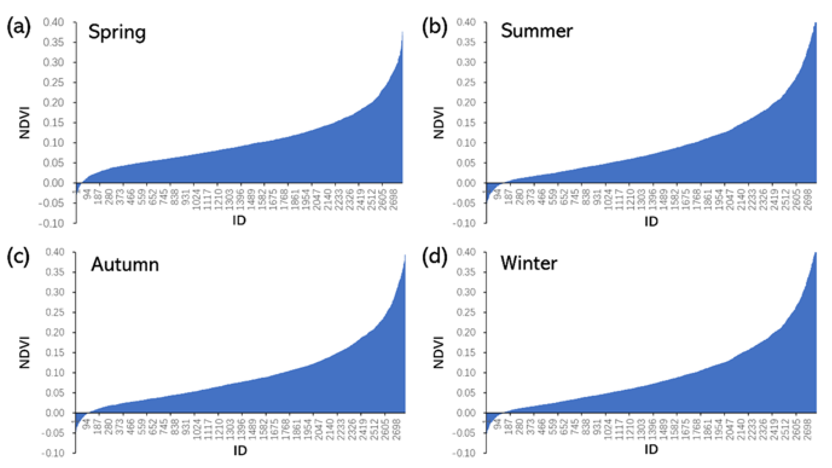
Based on the analysis in Section 5.3 that the correlation between UHM and each variable is significant and there is no multicollinearity, it presents established multivariate regressions used to estimate UHMs in built-up areas (denoted by UHMB) and land-cover areas (denoted by UHML) in four seasons (i.e., Equations (16)–(19) for spring, Equations (20)–(23) for summer, Equations (24)–(27) for autumn, and Equations (28)–(31) for winter), where X1 (Equation (14)) and X2 (Equation (15)) are two matrices for land-use LCZs. The correlation trends revealed by PR in Table 5 and Table 6 are consistent with the coefficient matrices of C1 and C2. The regressions show that NDBI and NDVI are two indicators that significantly increase UHMs in the built-up LCZs, as the two corresponding coefficients are significantly larger than the others. The results also reveal that SVF and ASR are two important factors that cause UHIs during the daytime, which is different from UHIs formed by longwave emission from the ground at night [52,73]. Notably, the NDVI coefficient for UHMB is positive but the coefficient for UHML is negative. This is because NDVI values are low in built-up LCZs (Figure 8) that represent barren soil but high in land-cover LCZs that correspond to vegetation, resulting in an inverse influence on UHMs.
X1 = [NDBI NDVI SVF ASR BH FAR]
X2 = [LCZ-2 LCZ-3 LCZ-4 LCZ-8 LCZ-10]
C1 = [17.959 8.542 −0.778 0.438 −0.001 1.657 × 10⁻⁵]T
C2 = [0.224 0.554 −0.084 −1.013 0.568] T
UHMB = C1X1 + C2X2 + 1.194
UHML = −9.159NDVI + 0.733ASR + 0.947
C3 = [11.947 4.365 −0.714 0.559 −0.002 0.004]T
C4 = [0.291 0.479 −0.203 −1.463 0.426]T
UHMB = C3X1 + C4X2 + 2.603
UHML = −10.492NDVI + 0.642ASR + 2.203
C5 = [13.720 4.192 0.509 0.286 −0.003 0.001]T
C6 = [0.242 0.291 −0.171 −0.326 0.526]T
UHMB = C5X1 + C6X2 + 1.651
UHML = −10.205NDVI + 0.790ASR + 1.822
C7 = [18.134 7.781 0.393 0.962 −0.001 0.001]T
C8 = [0.436 0.527 −0.229 −0.069 0.556]T
UHMB = C7X1 + C8X2 + 0.374
UHML = −9.521NDVI + 1.331ASR + 0.954
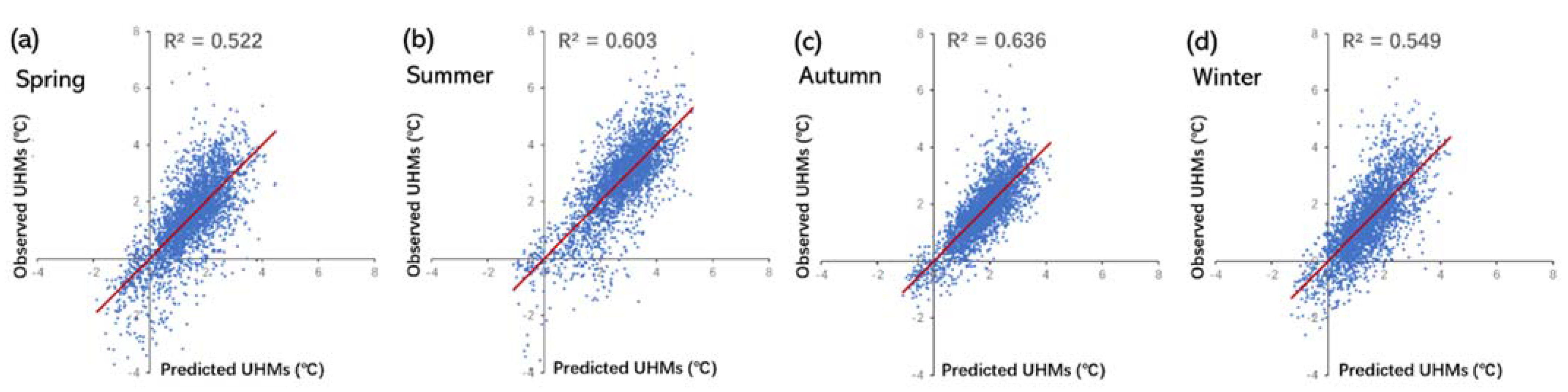
Figure 9 presents the predicted and observed UHMs for the whole study area with 3048 samples. It demonstrates that the red linear regression lines are almost on the diagonal with R2 values equaling 0.522, 0.603, 0.636, and 0.549 from spring to winter, indicating a reasonable predicting accuracy. The corresponding RMSE equals 0.912, 0.851, 0.621, and 0.836, which are also limited to 1 degree Celsius. Figure 10 depicts predicted UHM distributions that are quite similar to the observation as shown in Figure 5. Overall, they are spatially consistent and quantitatively close with each other across the entire Kowloon area, with a clear seasonal variation on the four days. Several UHM hotspots in specific urban areas, such as Kowloon East, Kowloon Tang, and Hung Hom, are successfully predicted in summer in Figure 10b. This means that, based on the proposed and determined indicators, the spatial regression models can estimate UHM distributions with reasonable accuracy in different seasons.
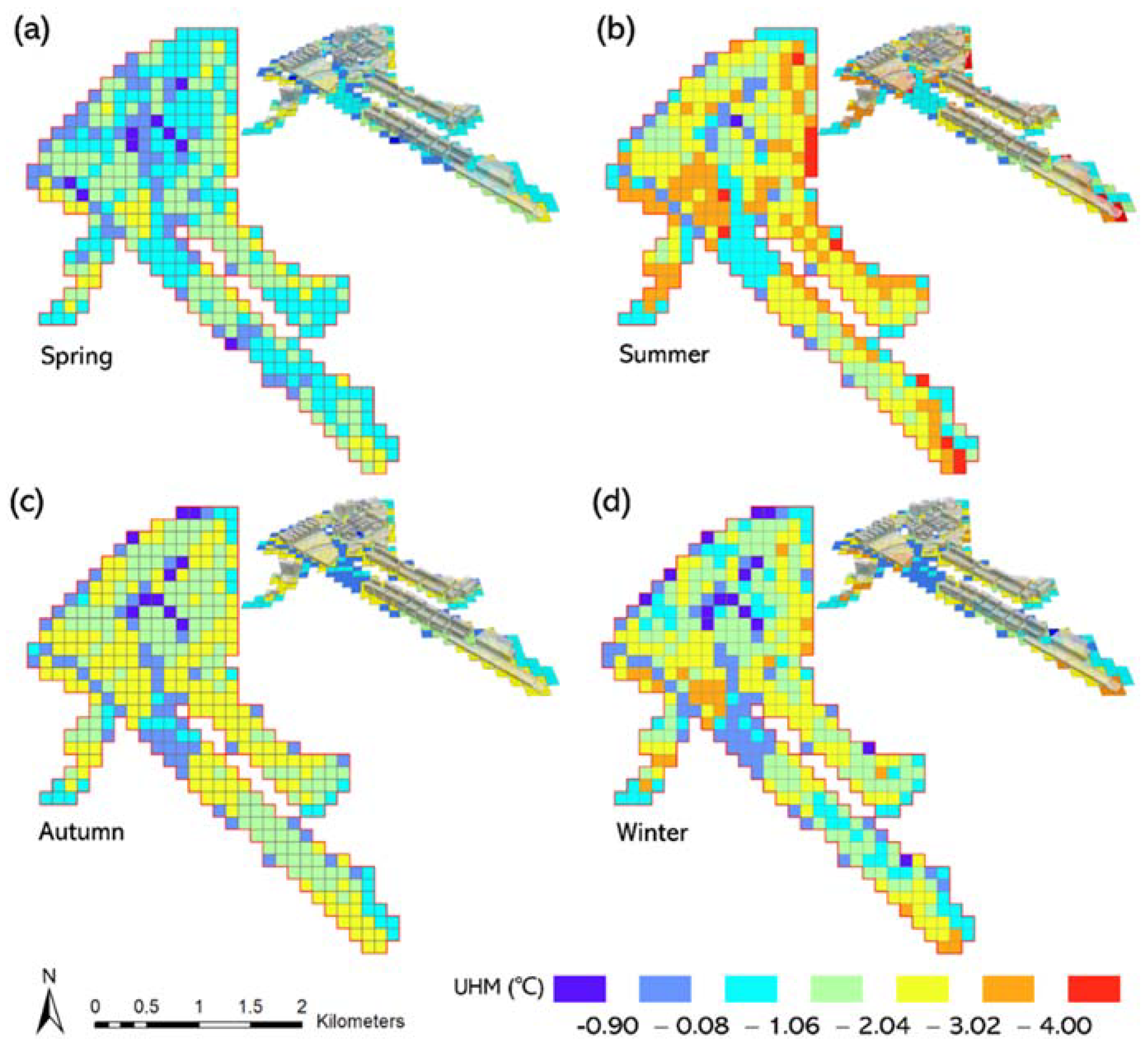
Based on the new LCZs in Figure 4a, SVF in Figure 4b, and ASR in Figure 6 that will occur in a transformed urban area and the established spatial regression models adaptive to four different seasons as presented in Equations (14)–(31), the distribution of UHMs with the same spatial resolution can be predicted on the four corresponding days in the Kowloon East area. In the future, the UHI effect will be most pronounced in summer in Figure 11b, followed by autumn in Figure 11c and winter in Figure 11d, and least pronounced in spring in Figure 11a. It is worth mentioning that the observed UHM on 14 November 2019 is overall 0.5 °C higher than on 20 August 2017, which makes the predicted UHMs in winter slightly larger than that in autumn. Nonetheless, in Kowloon East, the future UHMs based on the proposed master plan will be significantly lower across the four seasons when compared to either the observed UHMs (Figure 5) or estimated UHMs (Figure 10) based on the current urban landscape, resulting in obvious mitigation of the UHI effect. For instance, there will be only 12 grid cells with UHMs larger than 4 °C in summer in Figure 11b; while in winter, there will be several grid cells with UHMs lower than 0 °C in Figure 10d, revealing an urban heat sink phenomenon. The predicted UHM distribution suggests that the Government’s urban reform initiative will aid in the creation of a thermal-friendly urban environment.
7. Discussion and Conclusions
The forecasting of the UHM distributions based on a master plan of new buildings established by an urban reforming initiative in Kowloon East suggests that the UHI effect will be significantly mitigated compared to current UHMs. The main reason could be that this area will be transformed into an open space fulfilled with low plants that can effectively cool down LSTs, according to the future local climate zones. It is crucial to reveal that NDVI and ASR are the two most important indicators for explaining the daytime UHIs in both the built-up LCZs and land-cover LCZs. Furthermore, different LCZs have different effects on UHMs in the built-up area, indicating that microclimate can also be used to explain the UHI phenomenon. Although the values of R2 are not significantly high, the established models are accurate and reliable based on the evidence that the linear regressions between over 3000 observed and predicted samples have high consistency with the diagonal lines and the correlation is significant without multicollinearity.
This study established a framework for predicting UHMs based on a future urban landscape, which can effectively aid in urban planning to create a liveable urban environment. However, three limitations could have an impact on the estimation results. First, the spatial regression models are constantly based on a grid resolution of 100 m. This may result in a portion of the gird cells containing a mixture of LCZs, which challenges an accurate prediction of UHMs, particularly in densely populated areas. Second, heat generated by vehicle flows has not been incorporated into the model, which is supposed to be an unignorable heat source of UHIs during the daytime in Hong Kong [41]. Third, as the study area of Kowloon is a peninsula along the coast, cold wind from the sea may move along the ventilation corridors between buildings, thus creating a cooling effect on the UHI.
Future research can be conducted in four areas based on the proposed framework. First, both solar irradiation and traffic flow can be modelled as the heat source of UHI, and wind directions and intensities can be modelled by using computational fluid dynamic estimations and integrated into the proposed model as a new influential factor, which is especially important for Hong Kong, a city close to the coast. Second, with the availability of the thermal images captured during the nighttime, the nighttime UHI effect can be thoroughly investigated. Because the UHI formulation mechanism differs during the day and at night, this may result in different findings and effects from the indicators. Third, instead of building multivariate regression models, advanced machine learning (e.g., neural network regression and random forest) or deep learning methods (e.g., deep neural networks) can be used to construct a robust regression model to achieve high prediction accuracy. Fourth, further study can be directed toward optimizing the urban landscape to mitigate the UHI effect based on a throughout understanding of the UHI phenomenon and well-designed objective functions.
In conclusion, this study believes that solar irradiation, land use and land cover, urban morphology, and local climate zones can all have a significant impact on the daytime UHI phenomenon significantly. To estimate the future UHI effect in a reformed urban area, spatial multivariate regression models adaptive to different seasons are developed and tested. The prediction of the UHMs based on a master plan of new buildings suggests that a thermo-friendly urban environment can be expected in Kowloon East, Hong Kong. The proposed framework is useful for evaluating the UHI effect in urban planning and can be used by urban planners to improve the model for optimizing the urban landscape to further mitigate the UHI effect.
Author Contributions
Conceptualization, R.Z. and X.D.; methodology, R.Z. and X.D.; software, X.D.; validation, R.Z., X.D. and M.S.W.; visualization, X.D.; formal analysis, R.Z., X.D. and M.S.W.; writing, R.Z. and X.D.; review and editing, R.Z. and M.S.W.; supervision, M.S.W. All authors have read and agreed to the published version of the manuscript.
Funding
The authors thank the funding support from the Strategic Hiring Scheme (Grant No. P0036221) at the Hong Kong Polytechnic University; the Grant No. 1-CD81, Research Institute for Land and Space, The Hong Kong Polytechnic University; and General Research Fund (Grant No. 15602619 and 15603920), and Collaborative Research Fund (Grant No. C7064-18GF, C4023-20GF), from the Hong Kong Research Grants Council, Hong Kong, China.
Institutional Review Board Statement
Not applicable.
Informed Consent Statement
Not applicable.
Data Availability Statement
Not applicable.
Conflicts of Interest
The authors declare no conflict of interest.
References
- Landsberg, H.E. The Urban Climate; Academic Press: New York, NY, USA, 1981. [Google Scholar]
- Oke, T.R. City size and the urban heat island. Atmos. Environ. 1973, 7, 769–779. [Google Scholar] [CrossRef]
- Arnfield, A.J. Two decades of urban climate research: A review of turbulence, exchanges of energy and water, and the urban heat island. Int. J. Climatol. 2003, 23, 1–26. [Google Scholar] [CrossRef]
- Zhao, S.; Liu, S.; Zhou, D. Prevalent vegetation growth enhancement in urban environment. Proc. Natl. Acad. Sci. USA 2016, 113, 6313–6318. [Google Scholar] [CrossRef] [Green Version]
- Zhou, D.; Zhao, S.; Zhang, L.; Liu, S. Remotely sensed assessment of urbanization effects on vegetation phenology in China’s 32 major cities. Remote Sens. Environ. 2016, 176, 272–281. [Google Scholar] [CrossRef] [Green Version]
- Grimm, N.B.; Faeth, S.H.; Golubiewski, N.E.; Redman, C.L.; Wu, J.; Bai, X.; Briggs, J.M. Global Change and the Ecology of Cities. Science 2008, 319, 756–760. [Google Scholar] [CrossRef] [Green Version]
- Wang, Y.; Li, Y.; Di Sabatino, S.; Martilli, A.; Chan, P.W. Effects of anthropogenic heat due to air-conditioning systems on an extreme high temperature event in Hong Kong. Environ. Res. Lett. 2018, 13, 034015. [Google Scholar] [CrossRef]
- Rydin, Y.; Bleahu, A.; Davies, M.; Dávila, J.D.; Friel, S.; De Grandis, G.; Groce, N.; Hallal, P.C.; Hamilton, I.; Howden-Chapman, P.; et al. Shaping cities for health: Complexity and the planning of urban environments in the 21st century. Lancet 2012, 379, 2079–2108. [Google Scholar] [CrossRef] [Green Version]
- Mirzaei, P.A.; Haghighat, F. Approaches to study Urban Heat Island—Abilities and limitations. Build. Environ. 2010, 45, 2192–2201. [Google Scholar] [CrossRef]
- Oke, T.R.; Johnson, G.T.; Steyn, D.G.; Watson, I.D. Simulation of surface urban heat islands under ‘ideal’ conditions at night part 2: Diagnosis of causation. Bound. Layer Meteorol. 1991, 56, 339–358. [Google Scholar] [CrossRef]
- Zhou, D.; Xiao, J.; Bonafoni, S.; Berger, C.; Deilami, K.; Zhou, Y.; Frolking, S.; Yao, R.; Qiao, Z.; Sobrino, J.A. Satellite Remote Sensing of Surface Urban Heat Islands: Progress, Challenges, and Perspectives. Remote Sens. 2019, 11, 48. [Google Scholar] [CrossRef] [Green Version]
- Bokaie, M.; Zarkesh, M.K.; Arasteh, P.D.; Hosseini, A. Assessment of Urban Heat Island based on the relationship between land surface temperature and Land Use/Land Cover in Tehran. Sustain. Cities Soc. 2016, 23, 94–104. [Google Scholar] [CrossRef]
- Liang, X.; Ji, X.; Guo, N.; Meng, L. Assessment of urban heat islands for land use based on urban planning: A case study in the main urban area of Xuzhou City, China. Environ. Earth Sci. 2021, 80, 308. [Google Scholar] [CrossRef]
- Guo, G.; Wu, Z.; Xiao, R.; Chen, Y.; Liu, X.; Zhang, X. Impacts of urban biophysical composition on land surface temperature in urban heat island clusters. Landsc. Urban Plan. 2015, 135, 1–10. [Google Scholar] [CrossRef]
- Lin, P.; Lau, S.S.Y.; WIn, H.; Gou, Z. Effects of urban planning indicators on urban heat island: A case study of pocket parks in high-rise high-density environment. Landsc. Urban Plan. 2017, 168, 48–60. [Google Scholar] [CrossRef]
- Coseo, P.; Larsen, L. How factors of land use/land cover, building configuration, and adjacent heat sources and sinks explain Urban Heat Islands in Chicago. Landsc. Urban Plan. 2014, 125, 117–129. [Google Scholar] [CrossRef]
- Kotharkar, R.; Bagade, A.; Ramesh, A. Assessing urban drivers of canopy layer urban heat island: A numerical modeling approach. Landsc. Urban Plan. 2019, 190, 103586. [Google Scholar] [CrossRef]
- Chun, B.; Guldmann, J.M. Spatial statistical analysis and simulation of the urban heat island in high-density central cities. Landsc. Urban Plan. 2014, 125, 76–88. [Google Scholar] [CrossRef]
- Peng, F.; Wong, M.S.; Ho, H.C.; Nichol, J.; Chan, P.W. Reconstruction of historical datasets for analyzing spatiotemporal influence of built environment on urban microclimates across a compact city. Build. Environ. 2017, 123, 649–660. [Google Scholar] [CrossRef]
- Giridharan, R.; Lau, S.S.Y.; Ganesan, S.; Givoni, B. Urban design factors influencing heat island intensity in high-rise high-density environments of Hong Kong. Build. Environ. 2007, 42, 3669–3684. [Google Scholar] [CrossRef]
- Clinton, N.; Gong, P. MODIS detected surface urban heat islands and sinks: Global locations and controls. Remote Sens. Environ. 2013, 134, 294–304. [Google Scholar] [CrossRef]
- Shi, Y.; Xiang, Y.; Zhang, Y. Urban Design Factors Influencing Surface Urban Heat Island in the High-Density City of Guangzhou Based on the Local Climate Zone. Sensors 2019, 19, 3459. [Google Scholar] [CrossRef] [Green Version]
- Zha, Y.; Gao, J.; Ni, S. Use of normalized difference built-up index in automatically mapping urban areas from TM imagery. Int. J. Remote Sens. 2003, 24, 583–594. [Google Scholar] [CrossRef]
- Pal, S.; Ziaul, S. Detection of land use and land cover change and land surface temperature in English Bazar urban centre. Egypt. J. Remote Sens. Space Sci. 2017, 20, 125–145. [Google Scholar] [CrossRef] [Green Version]
- Wardlow, B.D.; Egbert, S.L.; Kastens, J.H. Analysis of time-series MODIS 250 m vegetation index data for crop classification in the U.S. Central Great Plains. Remote Sens. Environ. 2007, 108, 290–310. [Google Scholar] [CrossRef] [Green Version]
- Smoliak, B.V.; Snyder, P.K.; Twine, T.E.; Mykleby, P.M.; Hertel, W.F. Dense Network Observations of the Twin Cities Canopy-Layer Urban Heat Island. J. Appl. Meteorol. Climatol. 2015, 54, 1899–1917. [Google Scholar] [CrossRef]
- Yu, Z.; Yao, Y.; Yang, G.; Wang, X.; Vejre, H. Strong contribution of rapid urbanization and urban agglomeration development to regional thermal environment dynamics and evolution. For. Ecol. Manag. 2019, 446, 214–225. [Google Scholar] [CrossRef]
- Manoli, G.; Fatichi, S.; Schläpfer, M.; Yu, K.; Crowther, T.W.; Meili, N.; Burlando, P.; Katul, G.G.; Bou-Zeid, E. Magnitude of urban heat islands largely explained by climate and population. Nature 2019, 573, 55–60. [Google Scholar] [CrossRef]
- Liu, H.; Huang, B.; Zhan, Q.; Gao, S.; Li, R.; Fan, Z. The influence of urban form on surface urban heat island and its planning implications: Evidence from 1288 urban clusters in China. Sustain. Cities Soc. 2021, 71, 102987. [Google Scholar] [CrossRef]
- Icaza, L.E.; van den Dobbelsteen, A.V.; Hoeven, F.V. Integrating Urban Heat Assessment in Urban Plans. Sustainability 2016, 8, 320. [Google Scholar] [CrossRef] [Green Version]
- Zhu, R.; Guilbert, E.; Wong, M.S. Object-oriented tracking of the dynamic behavior of urban heat islands. Int. J. Geogr. Inf. Sci. 2017, 31, 405–424. [Google Scholar] [CrossRef] [Green Version]
- Zhu, R.; Guilbert, E.; Wong, M.S. Object-oriented tracking of spatial and thematic dynamic behaviors of urban heat islands. Trans. GIS 2020, 24, 85–103. [Google Scholar] [CrossRef]
- Zhang, Y.; Murray, A.T.; Turner, B.L., II. Optimizing green space locations to reduce daytime and nighttime urban heat island effects in Phoenix, Arizona. Landsc. Urban Plan. 2017, 165, 162–171. [Google Scholar] [CrossRef]
- Stewart, I.D.; Oke, T.R. Local Climate Zones for Urban Temperature Studies. Bull. Am. Meteorol. Soc. 2012, 93, 1879–1900. [Google Scholar] [CrossRef]
- Wang, K.; Jiang, S.; Wang, J.; Zhou, C.; Wang, X.; Lee, X. Comparing the diurnal and seasonal variabilities of atmospheric and surface urban heat islands based on the Beijing urban meteorological network. J. Geophys. Res. Atmos. 2017, 122, 2131–2154. [Google Scholar] [CrossRef]
- Deilami, K.; Kamruzzaman, M.; Liu, Y. Urban heat island effect: A systematic review of spatio-temporal factors, data, methods, and mitigation measures. Int. J. Appl. Earth Obs. Geoinf. 2018, 67, 30–42. [Google Scholar] [CrossRef]
- Weng, Q. Thermal infrared remote sensing for urban climate and environmental studies: Methods, applications, and trends. ISPRS J. Photogramm. Remote Sens. 2009, 64, 335–344. [Google Scholar] [CrossRef]
- Zhou, B.; Rybski, D.; Kropp, J.P. The role of city size and urban form in the surface urban heat island. Sci. Rep. 2017, 7, 4791. [Google Scholar] [CrossRef]
- Kwak, Y.; Park, C.; Deal, B. Discerning the success of sustainable planning: A comparative analysis of urban heat island dynamics in Korean new towns. Sustain. Cities Soc. 2020, 61, 102341. [Google Scholar] [CrossRef]
- Yin, C.; Yuan, M.; Lu, Y.; Huang, Y.; Liu, Y. Effects of urban form on the urban heat island effect based on spatial regression model. Sci. Total Environ. 2018, 634, 696–704. [Google Scholar] [CrossRef]
- Nassar, A.K.; Blackburn, G.A.; Whyatt, J.D. Dynamics and controls of urban heat sink and island phenomena in a desert city: Development of a local climate zone scheme using remotely-sensed inputs. Int. J. Appl. Earth Obs. Geoinf. 2016, 51, 76–90. [Google Scholar] [CrossRef] [Green Version]
- Zhu, R.; Wong, M.S.; Guilbert, E.; Chan, P.W. Understanding heat patterns produced by vehicular flows in urban areas. Sci. Rep. 2017, 7, 16309. [Google Scholar] [CrossRef] [Green Version]
- Leconte, F.; Bouyer, J.; Claverie, R.; Pétrissans, M.J.B. Using Local Climate Zone scheme for UHI assessment: Evaluation of the method using mobile measurements. Build. Environ. 2015, 83, 39–49. [Google Scholar] [CrossRef]
- Lelovics, E.; Unger, J.; Gál, T.; Gál, C.V. Design of an urban monitoring network based on Local Climate Zone mapping and temperature pattern modelling. Clim. Res. 2014, 60, 51–62. [Google Scholar] [CrossRef] [Green Version]
- Stewart, I.D.; Oke, T.R.; Krayenhoff, E.S. Evaluation of the ‘local climate zone’ scheme using temperature observations and model simulations. Int. J. Climatol. 2014, 34, 1062–1080. [Google Scholar] [CrossRef]
- Oguz, H. LST calculator: A program for retrieving land surface temperature from Landsat TM/ETM+ imagery. Environ. Eng. Manag. J. 2013, 12, 549–555. [Google Scholar] [CrossRef]
- Zareie, S.; Khosravi, H.; Nasiri, A. Derivation of land surface temperature from Landsat Thematic Mapper (TM) sensor data and analyzing relation between land use changes and surface temperature. Solid Earth Discuss 2016, 1–15. [Google Scholar] [CrossRef]
- Ihlen, V. Landsat 8 Data Users Handbook; US Geological Survey: Sioux Falls, SD, USA, 2019; p. 55.
- Chen, X.L.; Zhao, H.M.; Li, P.X.; Yin, Z.Y. Remote sensing image-based analysis of the relationship between urban heat island and land use/cover changes. Remote Sens. Environ. 2006, 104, 133–146. [Google Scholar] [CrossRef]
- Javadnia, E.; Mobasheri, M.R.; Kamali, G.H.A. MODIS NDVI quality enhancement using ASTER images. J. Agric. Sci. Technol. 2009, 11, 549–558. [Google Scholar]
- Townshend, J.R.G.; Justice, C.O. Analysis of the dynamics of African vegetation using the normalized difference vegetation index. Int. J. Remote Sens. 1986, 7, 1435–1445. [Google Scholar] [CrossRef]
- Watson, I.D.; Johnson, G.T. Graphical estimation of sky view-factors in urban environments. J. Climatol. 1987, 7, 193–197. [Google Scholar] [CrossRef]
- Chen, Q.; Cheng, Q.; Chen, Y.; Li, K.; Wang, D.; Cao, S. The Influence of Sky View Factor on Daytime and Nighttime Urban Land Surface Temperature in Different Spatial-Temporal Scales: A Case Study of Beijing. Remote Sens. 2021, 13, 4117. [Google Scholar] [CrossRef]
- Bernard, J.; Bocher, E.; Petit, G.; Palominos, S. Sky view factor calculation in urban context: Computational performance and accuracy analysis of two open and free GIS Tools. Climate 2018, 6, 60. [Google Scholar] [CrossRef] [Green Version]
- Fu, P.; Rich, P.M. A geometric solar radiation model with applications in agriculture and forestry. Comput. Electron. Agric. 2002, 37, 25–35. [Google Scholar] [CrossRef]
- ESRI. Available online: https://desktop.arcgis.com/en/arcmap/10.3/tools/spatial-analyst-toolbox/area-solar-radiation.htm (accessed on 8 August 2021).
- Huang, S.; Rich, P.M.; Crabtree, R.L.; Potter, C.S.; Fu, P. Modeling Monthly Near-Surface Air Temperature from Solar Radiation and Lapse Rate: Application over Complex Terrain in Yellowstone National Park. Phys. Geogr. 2008, 29, 158–178. [Google Scholar] [CrossRef]
- Census and Statistics Department. Available online: https://www.bycensus2016.gov.hk/tc/index.html (accessed on 8 August 2021).
- Lands Department. Available online: https://www.landsd.gov.hk/tc/resources/mapping-information/hk-geographic-data.html (accessed on 8 August 2021).
- Energizing Kowloon East Office. Available online: https://www.ekeo.gov.hk/en/home/index.html (accessed on 8 August 2021).
- Nichol, J.E.; Fung, W.Y.; Lam, K.; Wong, M.S. Urban heat island diagnosis using ASTER satellite images and ‘in situ’ air temperature. Atmos. Res. 2009, 94, 276–284. [Google Scholar] [CrossRef]
- Wong, M.S.; Peng, F.; Zou, B.; Shi, W.Z.; Wilson, G.J. Spatially analyzing the inequity of the Hong Kong urban heat island by socio-demographic characteristics. Int. J. Environ. Res. Public Health 2016, 13, 317. [Google Scholar] [CrossRef] [Green Version]
- Hong Kong Observatory. Available online: https://www.weather.gov.hk/en/wxinfo/pastwx/mws/mws.htm (accessed on 8 August 2021).
- World Weather Online. Available online: https://www.worldweatheronline.com/hung-hom-weather-history/hk.aspx (accessed on 8 August 2021).
- United States Geological Survey. Available online: https://earthexplorer.usgs.gov/ (accessed on 8 August 2021).
- Town Planning Board. Available online: https://www2.ozp.tpb.gov.hk/gos/default.aspx (accessed on 8 August 2021).
- World Urban Database Portal Tools. Available online: https://wudapt.cs.purdue.edu/wudaptTools/default/cities (accessed on 8 August 2021).
- Development Bureau. Available online: https://www.ekeo.gov.hk/filemanager/ekeo/common/Smart-Green-Resilient-CBD/1106_Brenda_Au_ppt_WorldGBC_Congress_2015_Final.pdf (accessed on 8 August 2021).
- Mason, R.L.; Gunst, R.F.; Hess, J.L. Statistical Design and Analysis of Experiments: Applications to Engineering and Science; Wiley: New York, NY, USA, 1989. [Google Scholar]
- Menard, S. Applied Logistic Regression Analysis, 2nd ed.; SAGE Publications Inc.: Thousand Oaks, CA, USA, 1995. [Google Scholar]
- Huang, G.; Cadenasso, M. People, landscape, and urban heat island: Dynamics among neighborhood social conditions, land cover and surface temperatures. Landsc. Ecol. 2016, 31, 2507–2515. [Google Scholar] [CrossRef]
- Zhou, J.; Chen, Y.; Zhang, X.; Zhan, W. Modelling the diurnal variations of urban heat islands with multi-source satellite data. Int. J. Remote Sens. 2013, 34, 7568–7588. [Google Scholar] [CrossRef]
- Guo, J.; Han, G.; Xie, Y.; Cai, Z.; Zhao, Y. Exploring the relationships between urban spatial form factors and land surface temperature in mountainous area: A case study in Chongqing city, China. Sustain. Cities Soc. 2020, 61, 102286. [Google Scholar] [CrossRef]
Figure 1.
Research framework for estimating the UHMs in a planned urban area.

Figure 2.
The study area in the Kowloon district of Hong Kong.

Figure 3.
Spatial variations of LCZs and SVF for the current urban form in Kowloon. (a) Spatial distribution of the eleven identified LCZs; (b) Spatial distribution of SVFs.
Figure 3.
Spatial variations of LCZs and SVF for the current urban form in Kowloon. (a) Spatial distribution of the eleven identified LCZs; (b) Spatial distribution of SVFs.

Figure 4.
Spatial variations of LCZs and SVF for the planned urban form in Kowloon. (a) Spatial distribution of the eleven identified LCZs; (b) Spatial distribution of SVFs.
Figure 4.
Spatial variations of LCZs and SVF for the planned urban form in Kowloon. (a) Spatial distribution of the eleven identified LCZs; (b) Spatial distribution of SVFs.

Figure 5.
UHM distribution on four representative days corresponding to four seasons in Kowloon, Hong Kong. (a–d) Spring, Summer, Autumn, and Winter.
Figure 5.
UHM distribution on four representative days corresponding to four seasons in Kowloon, Hong Kong. (a–d) Spring, Summer, Autumn, and Winter.

Figure 6.
Area solar irradiation in Kowloon East based on the building master plan. (a–d) Spring, Summer, Autumn, and Winter.
Figure 6.
Area solar irradiation in Kowloon East based on the building master plan. (a–d) Spring, Summer, Autumn, and Winter.

Figure 7.
Boxplots of the six indicators categorized by LCZs in summer. (a–f) NDBI, NDVI, SVF, SAR, DEN, and FAR.
Figure 7.
Boxplots of the six indicators categorized by LCZs in summer. (a–f) NDBI, NDVI, SVF, SAR, DEN, and FAR.

Figure 8.
An ascending order of the NDVI (in the y-axis) subject to grid cell ID (in the x-axis) in the land-use LCZs. (a–d) Spring, Summer, Autumn, and Winter.
Figure 8.
An ascending order of the NDVI (in the y-axis) subject to grid cell ID (in the x-axis) in the land-use LCZs. (a–d) Spring, Summer, Autumn, and Winter.

Figure 9.
The observed and predicted UHMs. (a–d) Spring, Summer, Autumn, and Winter.

Figure 10.
Spatial distribution of the predicted UHMs. (a–d) Spring, Summer, Autumn, and Winter.

Figure 11.
Estimated UHMs in Kowloon East based on the building master plan. (a–d) Spring, Summer, Autumn, and Winter.
Figure 11.
Estimated UHMs in Kowloon East based on the building master plan. (a–d) Spring, Summer, Autumn, and Winter.


Table 1.
Statistics of the identified LCZs.
| Types | Zones | Description | Counts | Proportion |
|---|---|---|---|---|
| Built-up types | LCZ-1 | Compact highrise | 590 | 19.36% |
| LCZ-2 | Compact midrise | 569 | 18.67% | |
| LCZ-3 | Compact lowrise | 237 | 7.78% | |
| LCZ-4 | Open highrise | 797 | 26.15% | |
| LCZ-5 | Open midrise | 85 | 2.79% | |
| LCZ-6 | Open lowrise | 5 | 0.16% | |
| LCZ-8 | Large lowrise | 225 | 7.38% | |
| LCZ-10 | Heavy industry | 264 | 8.66% | |
| Land-cover types | LCZ-A | Dense trees | 70 | 2.30% |
| LCZ-D | Low plants | 59 | 1.94% | |
| LCZ-E | Bare rock or paved | 147 | 4.82% |
Table 2.
Statistics of the future LCZs.
| Type | Zone | Description | Count | Proportion |
|---|---|---|---|---|
| Built-up type | LCZ-4 | Open highrise | 102 | 27.27% |
| LCZ-5 | Open midrise | 51 | 13.64% | |
| LCZ-6 | Open lowrise | 124 | 33.15% | |
| Land-cover type | LCZ-D | Low plants | 97 | 25.94% |
Table 3.
Atmospheric condition corresponding to the dates of the Landsat-8 imagery.
| Seasons | Dates | Radiation Parameters | |
|---|---|---|---|
| Transmittivity | Diffuse Proportion | ||
| Spring | 1 April 2018 | 0.62 | 0.30 |
| Summer | 20 August 2017 | 0.70 | 0.20 |
| Autumn | 14 November 2019 | 0.70 | 0.20 |
| Winter | 2 December 2020 | 0.62 | 0.30 |
Table 4.
Summary of the linear regressions between UHM and the eight indicators.
| Season | Coef. | NDBI | NDVI | SVF | ASR | DEN | FAR | OSR | BH |
|---|---|---|---|---|---|---|---|---|---|
| Spring | R | 0.5500 | −0.1930 | 0.0240 | 0.2570 | 0.0540 | 0.0060 | 0.0100 | −0.1000 |
| PR | 0.561 | 0.386 | −0.119 | 0.084 | 0.078 | −0.020 | 0.010 | −0.065 | |
| p | 0.0000 | 0.0000 | 0.0000 | 0.0000 | 0.0000 | 0.0000 | 0.5870 | 0.2800 | |
| O | 0.288 | 0.293 | 0.275 | 0.275 | 0.142 | 0.619 | 0.993 | 0.131 | |
| VIF | 3.467 | 3.409 | 3.632 | 3.631 | 7.024 | 1.615 | 1.007 | 7.616 | |
| Summer | R | 0.6200 | −0.4780 | −0.1510 | 0.1520 | 0.2250 | 0.1260 | 0.0140 | −0.0550 |
| PR | 0.397 | 0.138 | −0.167 | 0.243 | 0.168 | 0.040 | 0.048 | −0.146 | |
| p | 0.0000 | 0.0000 | 0.0000 | 0.0000 | 0.0000 | 0.0000 | 0.0080 | 0.0270 | |
| O | 0.194 | 0.199 | 0.289 | 0.364 | 0.178 | 0.520 | 0.995 | 0.148 | |
| VIF | 5.154 | 5.026 | 3.464 | 2.751 | 5.611 | 1.922 | 1.005 | 6.742 | |
| Autumn | P | 0.6930 | −0.4030 | 0.0960 | 0.2170 | 0.0750 | 0.0000 | 0.0110 | −0.1970 |
| PR | 0.618 | 0.236 | 0.054 | 0.058 | 0.146 | −0.062 | 0.032 | −0.122 | |
| p | 0.0000 | 0.0000 | 0.0030 | 0.0010 | 0.0000 | 0.0000 | 0.0780 | 0.0010 | |
| O | 0.284 | 0.251 | 0.262 | 0.267 | 0.142 | 0.619 | 0.992 | 0.131 | |
| VIF | 3.517 | 3.987 | 3.811 | 3.74 | 7.036 | 1.614 | 1.008 | 7.637 | |
| Winter | R | 0.5000 | −0.2670 | 0.2130 | 0.3300 | −0.0130 | −0.0980 | 0.0320 | −0.2020 |
| PR | 0.540 | 0.313 | 0.053 | 0.182 | 0.149 | 0.025 | 0.049 | −0.133 | |
| p | 0.0000 | 0.0000 | 0.0030 | 0.0000 | 0.0000 | 0.0000 | 0.0060 | 0.1670 | |
| O | 0.183 | 0.169 | 0.234 | 0.255 | 0.179 | 0.512 | 0.995 | 0.146 | |
| VIF | 5.457 | 5.933 | 4.271 | 3.929 | 5.601 | 1.955 | 1.005 | 6.846 |
Table 5.
Correlations between UHMs and the indicators for built-up LCZs.
| Season | Coef. | NDBI | NDVI | SVF | ASR | BH | FAR | LCZ-2 | LCZ-3 | LCZ-4 | LCZ-8 | LCZ-10 |
|---|---|---|---|---|---|---|---|---|---|---|---|---|
| Spring | R | 0.457 | 0.001 | 0.071 | 0.286 | −0.138 | −0.038 | 0.075 | 0.194 | −0.162 | −0.201 | 0.232 |
| PR | 0.499 | 0.324 | −0.060 | 0.139 | −0.032 | 0.000 | 0.081 | 0.144 | −0.027 | −0.212 | 0.145 | |
| p | 0.000 | 0.000 | 0.000 | 0.000 | 0.000 | 0.023 | 0.000 | 0.000 | 0.000 | 0.000 | 0.000 | |
| O | 0.373 | 0.299 | 0.258 | 0.285 | 0.648 | 0.743 | 0.679 | 0.748 | 0.441 | 0.520 | 0.658 | |
| VIF | 2.682 | 3.346 | 3.874 | 3.506 | 1.543 | 1.346 | 1.473 | 1.337 | 2.266 | 1.924 | 1.519 | |
| Summer | R | 0.522 | −0.304 | −0.102 | 0.154 | −0.127 | 0.073 | 0.204 | 0.196 | −0.357 | −0.219 | 0.254 |
| PR | 0.430 | 0.201 | −0.063 | 0.250 | −0.057 | 0.034 | 0.114 | 0.136 | −0.074 | −0.326 | 0.120 | |
| p | 0.000 | 0.000 | 0.000 | 0.000 | 0.000 | 0.000 | 0.000 | 0.000 | 0.000 | 0.000 | 0.000 | |
| O | 0.210 | 0.199 | 0.278 | 0.377 | 0.660 | 0.741 | 0.674 | 0.747 | 0.463 | 0.526 | 0.660 | |
| VIF | 4.752 | 5.017 | 3.592 | 2.650 | 1.516 | 1.350 | 1.484 | 1.339 | 2.158 | 1.901 | 1.516 | |
| Autumn | R | 0.584 | −0.207 | 0.182 | 0.333 | −0.276 | −0.065 | 0.110 | 0.169 | −0.342 | 0.032 | 0.299 |
| PR | 0.560 | 0.263 | 0.058 | 0.109 | −0.107 | 0.013 | 0.130 | 0.114 | −0.084 | −0.102 | 0.198 | |
| p | 0.000 | 0.000 | 0.000 | 0.000 | 0.000 | 0.000 | 0.000 | 0.000 | 0.000 | 0.048 | 0.000 | |
| O | 0.351 | 0.256 | 0.247 | 0.269 | 0.657 | 0.742 | 0.679 | 0.752 | 0.450 | 0.503 | 0.652 | |
| VIF | 2.851 | 3.910 | 4.053 | 3.722 | 1.522 | 1.347 | 1.472 | 1.331 | 2.222 | 1.988 | 1.533 | |
| Winter | R | 0.382 | −0.096 | 0.286 | 0.433 | −0.249 | −0.098 | 0.097 | 0.159 | −0.272 | 0.115 | 0.237 |
| PR | 0.481 | 0.338 | 0.033 | 0.212 | −0.039 | 0.013 | 0.175 | 0.155 | −0.086 | −0.017 | 0.159 | |
| p | 0.000 | 0.000 | 0.000 | 0.000 | 0.000 | 0.000 | 0.000 | 0.000 | 0.000 | 0.000 | 0.000 | |
| O | 0.227 | 0.183 | 0.235 | 0.259 | 0.661 | 0.740 | 0.678 | 0.755 | 0.464 | 0.512 | 0.654 | |
| VIF | 4.406 | 5.476 | 4.260 | 3.868 | 1.513 | 1.351 | 1.474 | 1.325 | 2.155 | 1.952 | 1.529 |
Table 6.
Correlations between UHMs and the indicators for land-cover LCZs.
| Date | Indicator | R | PR | p | O | VIF |
|---|---|---|---|---|---|---|
| Spring | NDVI | −0.852 | −0.776 | 0.000 | 0.688 | 1.453 |
| ASR | 0.644 | 0.388 | 0.000 | 0.688 | 1.453 | |
| Summer | NDVI | −0.889 | −0.803 | 0.000 | 0.591 | 1.692 |
| ASR | 0.696 | 0.363 | 0.000 | 0.591 | 1.692 | |
| Autumn | NDVI | −0.907 | −0.910 | 0.000 | 0.959 | 1.043 |
| ASR | 0.339 | 0.376 | 0.000 | 0.959 | 1.043 | |
| Winter | NDVI | −0.834 | −0.832 | 0.000 | 0.958 | 1.044 |
| ASR | 0.353 | 0.338 | 0.000 | 0.958 | 1.044 |
Publisher’s Note: MDPI stays neutral with regard to jurisdictional claims in published maps and institutional affiliations. |
© 2022 by the authors. Licensee MDPI, Basel, Switzerland. This article is an open access article distributed under the terms and conditions of the Creative Commons Attribution (CC BY) license (https://creativecommons.org/licenses/by/4.0/).
Share and Cite
MDPI and ACS Style
Zhu, R.; Dong, X.; Wong, M.S. Estimation of the Urban Heat Island Effect in a Reformed Urban District: A Scenario-Based Study in Hong Kong. Sustainability 2022, 14, 4409. https://0-doi-org.brum.beds.ac.uk/10.3390/su14084409
AMA Style
Zhu R, Dong X, Wong MS. Estimation of the Urban Heat Island Effect in a Reformed Urban District: A Scenario-Based Study in Hong Kong. Sustainability. 2022; 14(8):4409. https://0-doi-org.brum.beds.ac.uk/10.3390/su14084409
Chicago/Turabian StyleZhu, Rui, Xijia Dong, and Man Sing Wong. 2022. "Estimation of the Urban Heat Island Effect in a Reformed Urban District: A Scenario-Based Study in Hong Kong" Sustainability 14, no. 8: 4409. https://0-doi-org.brum.beds.ac.uk/10.3390/su14084409
Note that from the first issue of 2016, this journal uses article numbers instead of page numbers. See further details here.