Prediction of the Discharge Coefficient in Compound Broad-Crested-Weir Gate by Supervised Data Mining Techniques

Abstract

The current investigation evaluated the discharge coefficient of a combined compound rectangular broad-crested-weir (BCW) gate (C_dt) using the computational fluid dynamics (CFD) modeling approach and soft computing models. First, CFD was applied to the experimental data and 61 compound BCW gates were numerically simulated by resolving the Reynolds-averaged Navier–Stokes equations and stress turbulence models. Then, six data-driven procedures, including M5P tree, random forest (RF), support vector machine (SVM), Gaussian process (GP), multimode ANN and multilinear regression (MLR) were used for estimating the coefficient of discharge (C_dt) of the weir gates. The results showed the superlative accuracy of the SVM model compared to M5P, RF, GP and MLR in predicting the discharge coefficient. The sensitivity investigation revealed the h₁/H as the most effective parameter in predicting the C_dt, followed by the d/p, b/B₀, B/B₀ and z/p. The multimode ANN model reduced the root mean square error (RMSE) of M5P, RF, GP, SVM and MLR by 37, 13, 6.9, 6.5 and 32%, respectively. The graphical inspection indicated the multimode ANN model as the most suitable for predicting the C_dt of a BCW gate with minimum RMSE and maximum correlation.

1. Introduction

Hydrometry, which is the knowledge of assessing volumetric or hefty flow under pressure in open canals, is important for managing water resources. Various methods have been employed to measure flow in open channels, including pressure differences, hydraulic structures (flumes and weirs), velocity-area and tracer dilution [1,2,3]. Among these, gates and weirs are most widely used for flow measurement and discharge control in open canals [4,5]. The shape of the critical section and the upstream potential energy are the most effective parameters to determine the flow discharge in the crucial section (Dayev et al., 2021; Alkhatib and Gogus, 2014) [6,7]. Broad-crested weirs (BCW) can be used as dam channels and often as a dam. The BCW is a specially shaped weir (weir with a broad crest) designed to fit complex channel cross-sections [8]. The control section can also be shaped according to the range of variation of the discharge and head. Furthermore, the BCW, especially when the upstream side is inclined, can easily transmit the floating elements and sediment better than the sharp-crested weir [7]. Various investigations conducted on broad-crested weirs reported that the combined weir gate could adjust the upstream water level, flow control, and discharge measurement to meet agricultural needs [9,10,11,12,13]. According to Sakaruya and Kokpinar [14], the topmost benefit of a combined weir gate is the minimization and prevention of upstream sediment accumulation, which enhances the structure’s efficiency.

Several studies have been conducted to investigate the combined sharp-crested weir and gate [14,15,16,17,18]. Negm et al. [15] studied unrestricted flow over sharp-crested weirs and underneath gates. They investigated the effect of the geometrical and hydraulic parameters on the structures and reported that the rate of upstream water depth to gate opening (H/d) had major effects on the discharge. Ferro [19] presented discharge equations for a simple broad-crested-weir gate using incomplete self-similarity theory and dimensional analysis. Alhamid [16] investigated various combinations of weir-like gate proportions for both unrestricted and inundated flow and developed a discharge equation considering the effective parameters.

Soft computing approaches such as artificial intelligence (AI)-based models and multivariate analysis are widely employed in hydrology nowadays for decision-making [20,21,22,23,24,25,26,27,28,29]. The AI models have helped in the reduction in operation costs and time for decision-making rather than assessment through experimentation [30,31]. These techniques efficiently use the parameters and their backgrounds for problem estimation instead of merely resolving the prime equations [32,33]. Therefore, they can be used directly for resolving problems despite the many parameters and their interactions which create ambiguity and complexity in finding the solutions [25]. Discharge coefficient prediction using AI models has been successfully tested for triangular-labyrinth side weirs [34,35,36,37,38,39], semi-elliptical side weirs [40], trapezoidal-labyrinth side weirs [41,42,43,44,45,46], rectangular side weirs [47,48,49,50,51,52,53], and other types of weirs and gates [54,55,56,57,58,59]. However, the literature suggests that despite several existing acceptable techniques for estimating the discharge coefficient of hydraulic structures, the flow passing over a rectangular compound broad-crested-weir gate has not been considered using these techniques.

The main purpose of the present study was to develop new simple methods to predict this combined structure discharge coefficient (Cdt). The validated computational fluid dynamics (CFD) model was used to achieve this goal for a combined structure. This study proposed random forest (RF), M5P, support vector machine (SVM), genetic programming (GP), multilinear regression (MLR) and multimode artificial neural networks (ANN) to predict the C_dt in the compound BCW gate. All the effective parameters were changed to make different combinations of this structure. The BCW gate can be used as a flood control reservoir and a measuring device for minimizing the sediments and preventing their accumulation. An accurate prediction of the C_dt in the compound BCW gate could significantly improve its operational management and, thus, water resources management.

2. Theoretical Background

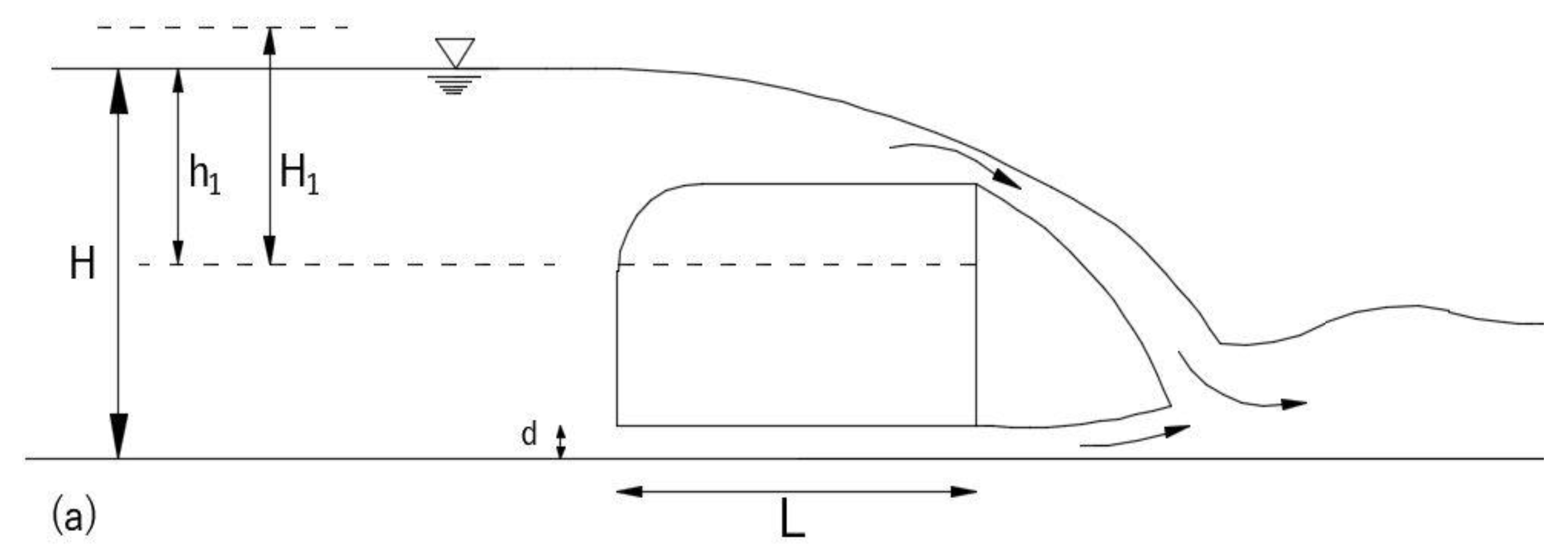
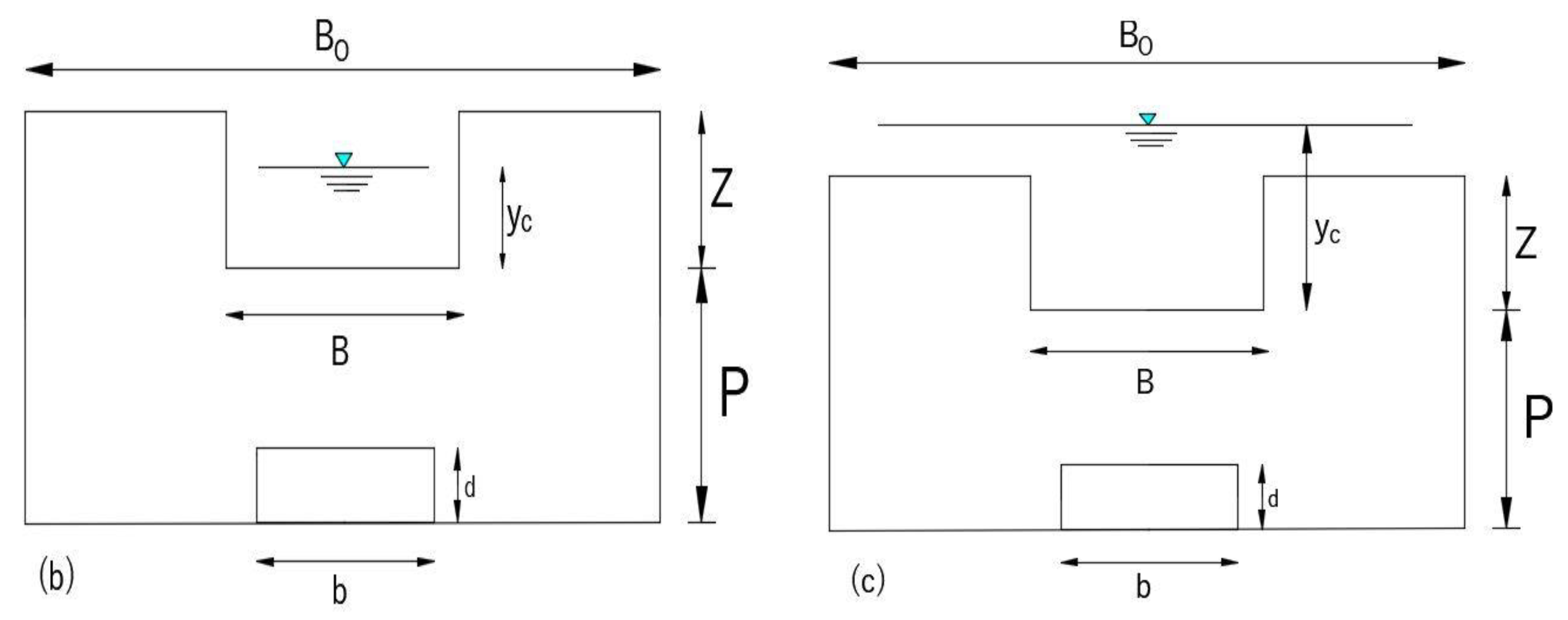
Figure 1a shows a rectangular, compound broad-crested weir. According to the upstream hydraulic head, there can be two cases. First, if the passage of the outlet discharge is only through the central weir (h₁ < Z) (Figure 1b), the broad-crested weir performs like a basic weir, and there will be no flow over the compound section.

In this case, the critical depth (y_c) will be lower than the central weir height (Z) and weir discharge (Q_w) though the broad-crested weir can be as follows [60,61];

$$Q_w=\frac{2}{3}{C}_{dw}{C}_{v}B{(\frac{2}{3}g)}^{1/2}{h_1}^{3/2}$$

(1)

where

$$C_{dw}=\frac{3}{2}\frac{Q}{B{(\frac{2}{3}g)}^{1/2}{H}_1^{3/2}}$$

(2)

$$C_v={(\frac{H_1}{h_1})}^{3/2}$$

(3)

where C_dw denotes the weir discharge coefficient, C_v denotes the weir velocity coefficient. Furthermore, h₁, g, B and H₁ are the water height above the central weir, acceleration gravity, central weir width and head overall energy at the weir head assessment section, respectively.

In another case, the water height above the central weir (h₁) surpasses the central weir height (Z), and the weir acts as a compound weir (Figure 1c). Furthermore, the critical flow depth (y_c) will be greater than the central weir height (Z). In this case, the BCW discharge (Q_w) is obtained by Equation (4) [5,61]:

$$Q_w=C_{dw}{C}_v{(\frac{g}{B_0})}^{1/2}{\left[BZ+B_0\left(\frac{2}{3}{h}_1-\frac{BZ}{3B_0}-\frac{2Z}{3}\right)\right]}^{3/2}$$

(4)

$$C_{dw}=\frac{Q_w}{{(\frac{g}{B_0})}^{1/2}{\left[BZ+B_0(\frac{2}{3}{H}_1-\frac{BZ}{3B_0}-\frac{2Z}{3})\right]}^{3/2}}$$

(5)

$$C_v={\left[\frac{BZ+B_0(\frac{2}{3}{H}_1-\frac{BZ}{3B_0}-\frac{2Z}{3})}{BZ+B_0(\frac{2}{3}{h}_1-\frac{BZ}{3B_0}-\frac{2Z}{3})}\right]}^{3/2}$$

(6)

Similarly, the equation of discharge pertaining to gates (Q_g) can be obtained by utilizing the equation of energy, as below [62]:

$$Q_g=c_{dg}db\sqrt{2gH}$$

(7)

where C_dg is the gate discharge coefficient and d, b and H are the gate opening height, gate breadth and level of upstream water, respectively. The investigation of the compound BCW and gate collectively for the two mentioned cases of compound BCW are elaborated below.

2.1. Case 1

As mentioned above, when the passage of outlet discharge is only via the central weir, the complex BCW performs as a basic weir. Thus, the combined structure (Figure 2b) discharge (Q_t) is the sum of Equation (1) and Equation (7) and can be written as Equation (8). The discharge coefficient for the combined compound BCW gate (C_dt) can be presented by Equation (9):

$$Q_t=Q_w+Q_g$$

(8)

$$C_{dt}=\frac{Q_t}{\frac{2}{3}{C}_{v}B{(\frac{2}{3}g)}^{1/2}{h}_1^{3/2}+db\sqrt{2gH}}$$

(9)

2.2. Case 2

When the passage of outlet discharge is through the compound section, the complex BCW can pass more water. Therefore, the discharge equation is different. In this case, the discharge related to the compound BCW gate (Q_t) (Figure 2c) is the sum of Equation (4) and Equation (7):

$$Q_t=Q_w+Q_g$$

(10)

$$C_{dt}=\frac{Q_t}{C_v{(\frac{g}{B_0})}^{1/2}{\left[BZ+B_0(\frac{2}{3}{h}_1-\frac{BZ}{3B_0}-\frac{2Z}{3})\right]}^{3/2}+db\sqrt{2gH}}$$

(11)

2.3. Governing Equations and Numerical Method

A three-dimensional CFD code was used to simulate a combined BCW–gate. The FLOW 3D code uses the finite volume scheme to resolve Reynolds-averaged Navier–Stokes (RANS) [63]. The Navier–Stokes equations are known as the equations of motion in fluid velocity mechanisms (u, v, w) in the three synchronous directions with some additional terms:

$$\begin{array}{l}\frac{\partial u}{\partial t}+\frac{1}{V_F}\left\{u{A}_x\frac{\partial u}{\partial x}+v{A}_{y}R\frac{\partial u}{\partial y}+w{A}_z\frac{\partial u}{\partial z}\right\}-\zeta \frac{A_y{v}^2}{x{V}_F}=-\frac{1}{\rho }\frac{\partial p}{\partial x}+G_x+f_x-b_x-\frac{R_{SOR}}{\rho V_F}(u-u_w-\delta u_s)\\ \frac{\partial v}{\partial t}+\frac{1}{V_F}\left\{u{A}_x\frac{\partial v}{\partial x}+v{A}_{y}R\frac{\partial v}{\partial y}+w{A}_z\frac{\partial v}{\partial z}\right\}-\zeta \frac{A_{y}uv}{x{V}_F}=-\frac{1}{\rho }(R\frac{\partial p}{\partial y})+G_y+f_y-b_y-\frac{R_{SOR}}{\rho V_F}(v-v_w-\delta v_s)\\ \frac{\partial w}{\partial t}+\frac{1}{V_F}\left\{u{A}_x\frac{\partial w}{\partial x}+v{A}_{y}R\frac{\partial w}{\partial y}+w{A}_z\frac{\partial w}{\partial z}\right\}=-\frac{1}{\rho }\frac{\partial p}{\partial z}+G_z+f_z-b_z-\frac{R_{SOR}}{\rho V_F}(w-w_w-\delta w_s)\end{array}$$

(12)

where G_x-z, f_x-z and b_x-z denote body accelerations, viscous accelerations and flow losses in porous media, respectively. Furthermore, A_x, A_y and A_z refer to the cross-sectional extent of the flow; ρ denotes the density of water, indicates the fractional volume open to flow in fractional area/volume obstacle representation (FAVOR), R_SOR denotes the source term, p denotes the pressure, and the concluding terms constitute the inclusion of mass at a source signified by a geometry component. The term U_w = (u_w, u_w, w_w) is the velocity of the source component, and the term U_s = (u_s, v_s, w_s) is the velocity at the surface of the source relative to the source itself. R in Equation (12) is the coefficient that depends on the choice of coordination system.

The volume of fluid (VOF) and FAVOR are the volume-fraction techniques employed for the condition of the depicting cell in the water surface and determination of the geometry, respectively [64]. Using this method, the CFD code enables us to ignore the surrounding air and its effect on the flowing water and create a sharp boundary between the air and water without the existence of fine interlocks [65,66,67]:

$$\frac{\partial F}{\partial t}+\frac{1}{v_f}\left[\frac{\partial }{\partial x}(F{A}_{X}u)+\frac{\partial }{\partial y}(F{A}_{y}v)+\frac{\partial }{\partial y}(F{A}_{z}w)\right]$$

(13)

Hirt and Sicilian [68] formulated the FAVOR method which is used to ascertain the level of the solid body inside an individual cell. In addition, this method can also determine the volume of cells unoccupied by a solid body. The CFD code used presents six turbulence models, including k−w, k−ε, RNG (the design is devised on R_e normalization groups with the equation of stress), one equation model, large-eddy simulation (LES) and the Prandtl mixing-length model [69].

3. Methods

The current investigation aimed to simulate a combined compound rectangular broad-crested-weir gate using FLOW-3D software. In order to do this, validation of numerical code was carried out using experimental results. The literature review indicated that the compound BCW-gate structure has not been studied before. Therefore, the experimental results of a single compound broad-crested weir by Salmasi et al., [12] were used for the calibration of CFD code. Salmasi et al. [12] experimentally studied a single broad-crested weir and estimated its properties, as given in

Table 1. Variables and their range used in the study of Salmasi et al., [12].

Parameters	L (cm)	B0 (cm)	B (cm)	p (cm)	Z (cm)
Range of variables	40	25	6, 8 and 12	10, 13 and 16	9

. To achieve the actual BCW, an attempt was made to deduce the relationship 0.1 < h₁/L ≤ 0.35 (where h₁ and L refer to the hydraulic head on the weir’s central section and the compound weir’s length, respectively) to establish the physical and arithmetic design [70]. The flow separation was decreased by rounding with a radius of 0.065 m at the weir entrance to develop physical and numerical models of the weir [5]. 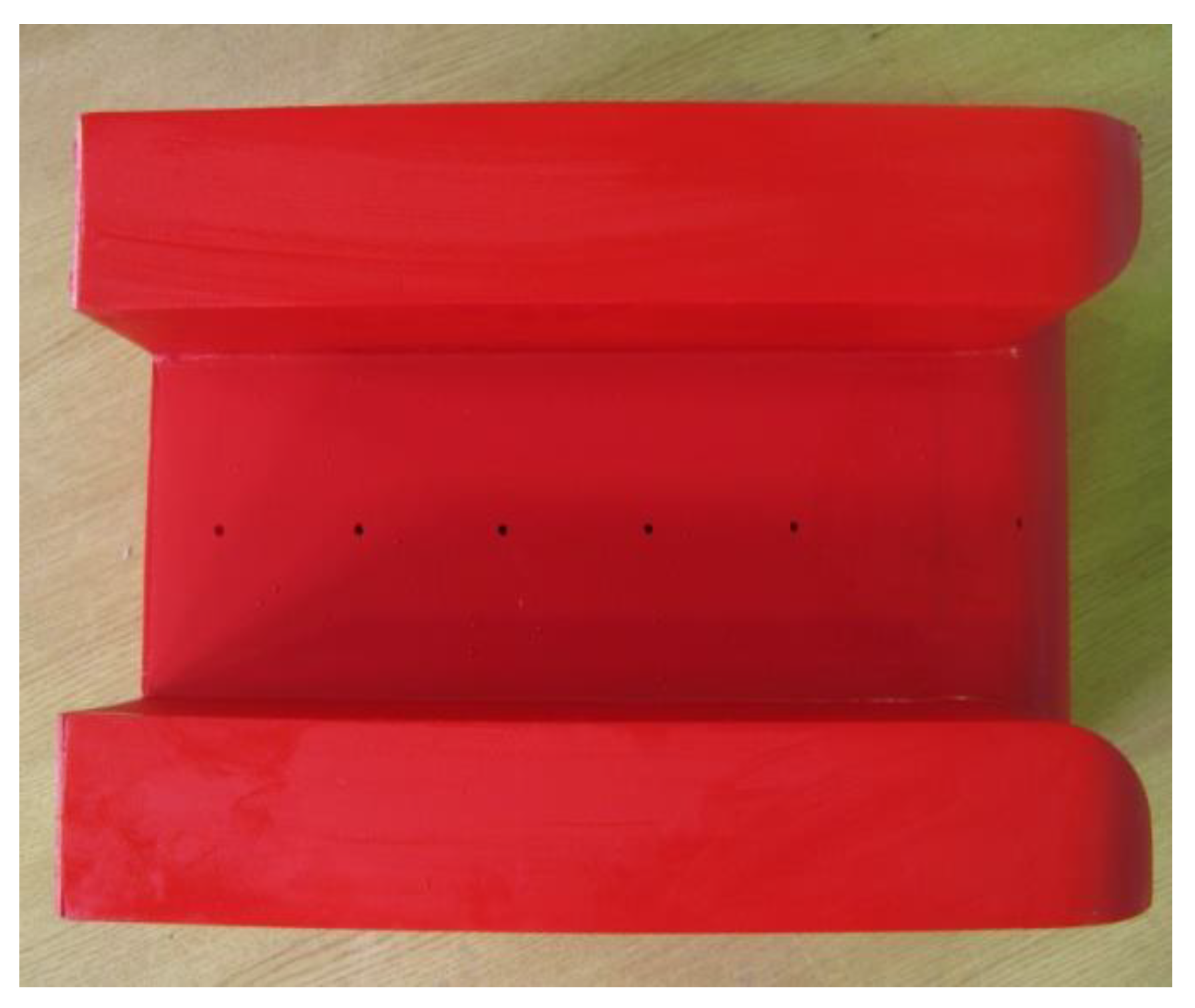Figure 3 shows the geometry of the experimental study conducted by Salmasi et al., [12].

To select a turbulence model with high accuracy based on the experimental results, the K–ω and RNG models’ outcomes were compared with those of the experimental measurements. Then, the most accurate model was used for the study. Instantaneous Navier–Stokes equations employing renormalization group theory were used to extract the RNG model [71]. For dissipation of the turbulent kinetic energy, the RNG two equations model uses an additional term in the transport equations [72]. The RNG equations appear as follows:

$$\frac{\partial }{\partial t}(\rho k)+\frac{\partial }{\partial x_i}(\rho k{u}_i)=\frac{\partial }{\partial x_j}\left[{\alpha }_k{\mu }_{eff}\frac{\partial k}{\partial x_j}\right]+G_k+G_b-\rho \epsilon -Y_M+S_k$$

(14)

$$\frac{\partial }{\partial t}(\rho \epsilon )+\frac{\partial }{\partial x_i}(\rho \epsilon u_i)=\frac{\partial }{\partial x_j}\left[{\alpha }_{\epsilon }{\mu }_{eff}\frac{\partial \epsilon }{\partial x_j}\right]+C_{1\epsilon }\frac{\epsilon }{k}(G_k+C_{3\epsilon }{G}_b)-C_{2\epsilon }\rho \frac{{\epsilon }^2}{k}-R_{\epsilon }+S_{\epsilon }$$

(15)

where K denotes kinetic energy, ε stands for rate of kinetic energy dissipation, ${\mu }_{eff}$ denotes effective viscosity, G_K and G_b stand for the generation of turbulent kinetic energy arising because of average velocity gradients and buoyancy, separately, Y_M is the fluctuating dilation in compressible turbulence, S_ε and S_K are the source terms set by the user, ${\alpha }_k$ and ${\alpha }_{\epsilon }$ are inverse effective Prandtl numbers for the turbulent kinetic energy and its dissipation, and $c_{1\epsilon }$, $c_{2\epsilon }$ and $c_{3\epsilon }$ are constants. Furthermore, the $R_{\epsilon }$ refers to the main difference between the numerical models used.

CFD code uses the standard k–w model. This empirical-based model was presented by Wilcox [73]. Because of its formulation, it is used for better computation of shear flow spreading the low Reynolds number’s effect and compressibility. Furthermore, transport equations are used in the k–w model for estimating turbulent kinetic energy (k) and its dissipation rate (w).

$$\frac{\partial }{\partial t}(\rho k)+\frac{\partial }{\partial x_i}(\rho k{u}_i)=\frac{\partial }{\partial x_i}\left[\left(\mu +\frac{{\mu }_t}{{\sigma }_k}\right)\frac{\partial k}{\partial x_j}\right]+G_k-Y_k+S_k$$

(16)

$$\frac{\partial }{\partial t}(\rho \omega )+\frac{\partial }{\partial x_i}(\rho \omega u_i)=\frac{\partial }{\partial x_j}\left[\left(\mu +\frac{{\mu }_t}{{\sigma }_{\omega }}\right)\frac{\partial \omega }{\partial x_j}\right]+G_{\omega }-Y_{\omega }+S_{\omega }$$

(17)

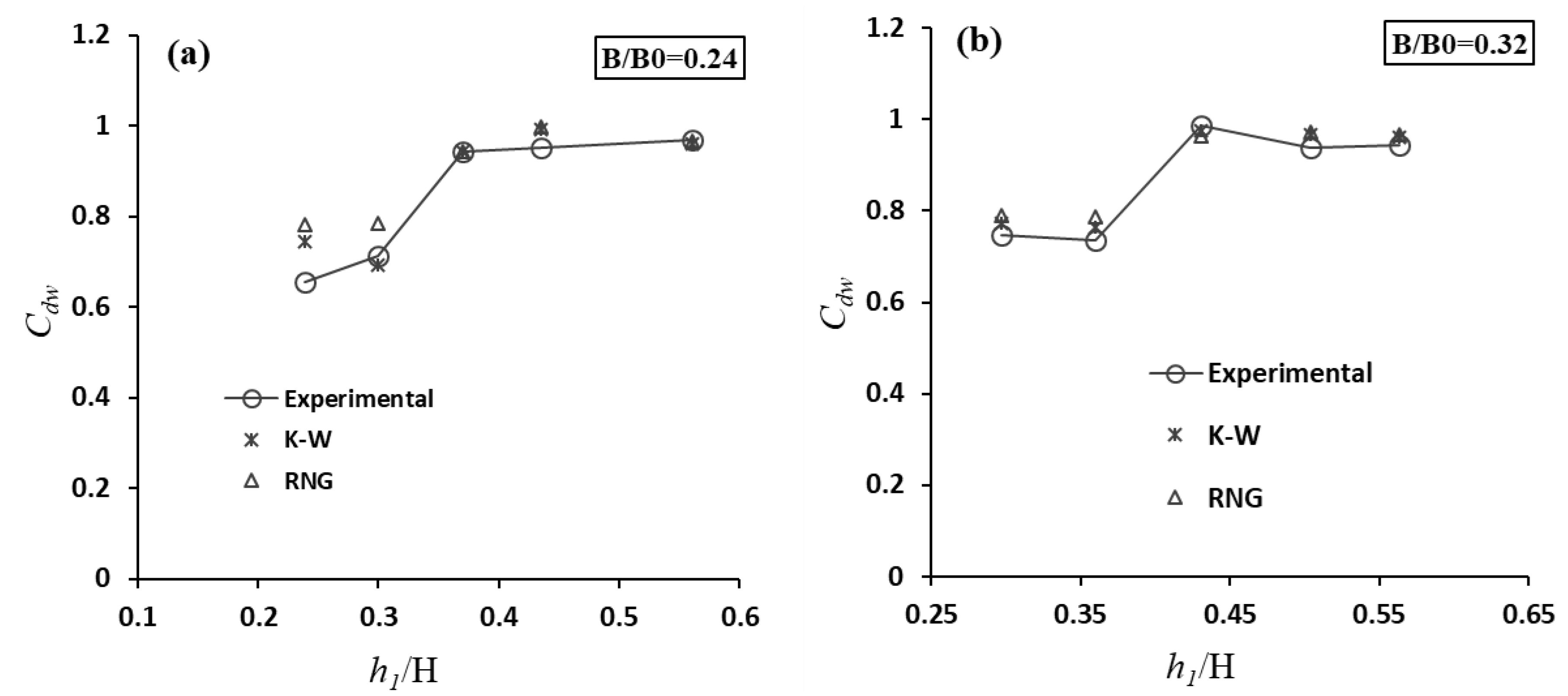
where $G_{\omega }$ is generation of ω, $Y_{\omega }$ is dissipation of ω due to turbulence, $Y_k$ is dissipation of k due to turbulence, ${\sigma }_{\omega }$ and ${\sigma }_k$ are the Prandtl number of turbulent (here they are constant; equal to 2), $S_{\omega }$ is the source term set by the user and ${\mu }_t$ is viscosity of turbulence. Figure 4 shows the results of RNG and k−w models in estimating C_dw.

Figure 4 shows that both models provide acceptable results in estimating C_dw and can be used to simulate a combined compound BCW gate. The root mean square (RMSE) values were 0.2685 for k-w against 0.3122 for RNG, when the k-w model was used for the simulation of the combined compound BCW-gate structure by CFD code.

The studied parameters were combined structure width, length and height (B₀, L, P + Z), central weir height and width (Z and B) and gate opening height and width (d and b). For upstream water level (H), different values were considered and two types of compound weir performance (simple weir and compound weir (Figure 2) were studied. Considering the mentioned parameters, the results are presented using dimensionless parameters. The structure’s total section width (B₀), the height of the structure (Z + P) and combined structure length (L) were considered as 0.25, 0.25 and 0.4, respectively.

Table 2. The studied dimensionless parameters and their values.

Parameters’ Values	Dimensionless Parameters
d/P	0.36, 0.43, 0.52, 0.62
b/B0	0.28, 0.4
Z/P	0.31, 0.56
B/Bo	0.24, 0.32, 0.48
h1/H	0.15, 0.2, 0.33, 0.42, 0.45, 0.54
d/P	0.36, 0.43, 0.52, 0.62

shows the studied dimensionless parameters and values.

Using these parameters, 61 numerical models were simulated using CFD code. For the arithmetic simulation, a grid of 1,200,000 elements was employed. After altering the mesh size and selecting the optimal size, the number of elements was selected. Specified pressure with specified water level and outflow was selected as X_min and X_max boundary conditions. Y_min, Y_max and Z_min were selected as boundary conditions. Furthermore, the symmetry was the Z_max boundary condition. Figure 5 shows one of the used models and its boundary conditions.

A constancy criterion such as the Courant number was used for temporal stage calculation. Both convergence criteria and stability were used to control the time step during the iterations. Flow kinetic energy monitoring was also used to survey the steady state condition. After calibration of CFD code with experimental results, k-w model was used to simulate the combined compound BCW gate. Combined structure discharge coefficients (C_dt) were generated using the simulation results for the two mentioned cases. Using the generated C_dt values, six soft computing-based models, including RF, M5P, SVM, GP, MLP and multimode ANN, were used to predict C_dt. The mentioned dimensionless parameters were the inputs of the soft computing models.

3.1. Soft Computing Models and Artificial Intelligence Techniques

3.1.1. M5P Model

M5P is a simple tree group technique for solving nonlinear and complex issues. This novel tree technique was introduced by Quinlan [74] for forecasting complex phenomena encompassing a huge quantity of datasets and variables. M5 tree is a piecewise simple model and takes a halfway situation between the linear and nonlinear designs [75]. Pruning is additionally associated with this technique to avoid overfitting. The separating technique is used at each node to accomplish higher information with minor deviation inside the subset down to the individual branch. This design has three significant advances: growth of tree, trimming and smoothing. Jothiprakash and Kote [76] explored the impact of trimming and smoothing and reported the favorable circumstances of unpruned and unsmoothed in hydrological studies. The tree model is created by unravelling the measures responsible for yielding standard deviation of the range class values to the nodes. In this strategy, linear connections are created at each node. Generally, it creates an excellent tree structure with a larger extent of precision.

3.1.2. Random Forest (RF)

RF, pioneered by Breiman [77], is widely used for resolving intricate engineering issues due to its flexibility. It employs a massive number of trees. The root nodes receive more diverse bootstrap (known as bagging) samples than the original data set. The assigned subset of the estimator parameters is unravelled randomly at the individual node. RF is simple, less training sensitive, yet meticulous in prediction [78]. Only two user-defined parameters: the number of trees grown (k) and the number of input parameters (m), are required. The formulation of this method employs a trial and error process. WEKA 3.9 software was used in this study for implementing RF.

3.1.3. Gaussian Process (GP)

GP is a set of random variables in which some variables have a multivariable Gaussian distribution. The chief objective of GP is to develop systems that can predict variables based on historical data. The uniqueness of GP lies in its specification through its mean and covariance function. It can be updated whenever new observational information is available [79]. GP depends on probability, which makes estimating input data easier and provides accuracy for probable variances. The statistical significance of the prediction is raised broadly by the estimated variances. GP can have vast dimensionality and produce data using the random domain of subset ranges. Choosing a suitable covariance function and its parameters is important because the main role of the GP belongs to the covariance function underlying the geometric structure of the training samples. The hyper-parameters (mean and covariance functions) must be determined from the data to improve accuracy [80,81,82].

3.1.4. Support Vector Machine (SVM)

SVM, a prevailing method in data mining, is a supervised-learning technique for solving regression and classification problems. It relies on the structural risk minimization principle [83,84,85]. SVM has been effectively used for linear and complex problems in various engineering and medical fields over the last few decades. Inadequate adjustment of user-defined constraints in SVM may result in overfitting and underfitting. To ascertain the best fit model, numerous trials were carried out to fix the user-defined parameters.

3.1.5. Multiple Linear Regression (MLR)

MLR employs the least square technique. The following is the equation of the MLR model:

$$R=c_0{x_1}^{c_1}{x_2}^{c_2}{x_3}^{c_3}{x_4}^{c_4}\dots {x_n}^{c_n}$$

(18)

where R stands for dependent variable and x₁, x₂,…_, x_n stand for independent variables. MLR was developed in this study using XLSTAT software.

3.1.6. Artificial Neural Networks (ANN)

The main benefit of ANN is its simplicity and ability to approximate any input/output [12]. The significant disadvantage of ANN techniques is that it shows information regarding the weight matrix that is currently beyond the discerning ability of human beings. In this way, normally, they are considered black box models. In addition, the ANN approach is aimed at finding user-defined parameters, such as the number of latent layers and neurons in latent layers, by trial and error, which is very time-consuming. The detailed theory about ANN occurs in Haykin [86]. Furthermore, the network is constrained by components, for example, learning rate, momentum, neuron numbers in layers and the number of hidden layers. Many trials were performed to find the best-fit model. The ANN was developed using the WEKA software. Figure 6 depicts the general structure of ANN with input, middle and output layers.

4. Application of the Methods

The prediction performance of the models was evaluated using the coefficient of correlation (CC), mean absolute error (MAE), root mean square error (RMSE), Nash–Sutcliffe model efficiency coefficient (Nash) and scattering index (SI) values, as defined below.

$$cc=\frac{n{\displaystyle \sum c_{d{t}_{obs}}{c}_{d{t}_{pred}-({\displaystyle \sum c_{d{t}_{obs}}})({\displaystyle \sum c_{d{t}_{pred}}})}}}{\sqrt{n{({\displaystyle \sum c_{d{t}_{obs}}})}^2-{({\displaystyle \sum c_{d{t}_{obs}}})}^2\sqrt{n{({\displaystyle \sum c_{d{t}_{pred}}})}^2-{({\displaystyle \sum c_{d{t}_{pred}}})}^2}}}$$

(19)

$$MAE=\frac{1}{n}\left|c_{d{t}_{obs}}-c_{d{t}_{pred}}\right|$$

(20)

$$RMSE=\sqrt{\frac{1}{N}({\displaystyle \sum _{i=1}^n{(c_{d{t}_{obs}}-c_{d{t}_{pred}})}^2)}}$$

(21)

$$Nash=1-\frac{{\displaystyle \sum _{i=1}^n{(c_{d{t}_{obs}}-c_{d{t}_{pred}})}^2}}{{\displaystyle \sum _{i=1}^n{(c_{d{t}_{obs}}-\overline{c_{d{t}_{obs}}})}^2}}$$

(22)

$$SI=\frac{RMSE}{c_{d{t}_{obs}}}$$

(23)

where $c_{d{t}_{obs}}$ is observed values, $c_{d{t}_{pred}}$ is predicted values, $\overline{c_{d{t}_{obs}}}$ is average observed values and n is the number of observations. If the values of CC and Nash Sutcliffe model efficiency are near 1, then the model is the best performing (if CC, Nash = 1, then the model is ideal). The lower values of MAE, RMSE and SI reflect the model’s suitability for prediction (if error is zero, then the model is ideal).

A total of 61 observations were used in this study for model development and validation. The models were constructed using 41 observations, whereas the remaining 20 observations were used for the testing. These groups were used for model development and validation.

Table 3. Features of the training and testing dataset.

Range	Training Data Set
	d/p	b/B0	Z/P	B/B0	h1/H	Cdt
Mean	0.4657	0.3502	0.4722	0.3629	0.3332	0.7945
Median	0.4375	0.4000	0.5625	0.3200	0.3333	0.8051
Standard deviation	0.0996	0.0599	0.1203	0.1045	0.1309	0.0800
Kurtosis	−0.9827	−1.9691	−1.7536	−1.7811	−1.2383	−0.1968
Skewness	0.7604	−0.3599	−0.5784	0.0931	0.0572	−0.6304
Minimum	0.3684	0.2800	0.3158	0.2400	0.1579	0.6155
Maximum	0.6250	0.4000	0.5625	0.4800	0.5429	0.9303
Confidence level (95.0%)	0.0314	0.0189	0.0380	0.0330	0.0413	0.0252
	Testing Data Set
Mean	0.4809	0.3520	0.4885	0.3600	0.3936	0.8188
Median	0.4375	0.4000	0.5625	0.3200	0.4286	0.8329
Standard deviation	0.1039	0.0603	0.1160	0.1054	0.1251	0.0748
Kurtosis	−1.4170	−2.0180	−1.2418	−1.8330	−0.5960	−1.2048
Skewness	0.5357	−0.4421	−0.9453	0.1533	−0.4966	−0.2163
Minimum	0.3684	0.2800	0.3158	0.2400	0.1579	0.6915
Maximum	0.6250	0.4000	0.5625	0.4800	0.5429	0.9235
Confidence level (95.0%)	0.0486	0.0282	0.0543	0.0493	0.0586	0.0350

summarizes the descriptive statistics of the training and testing phases, including maximum, minimum, standard deviation, mean, Kurtosis and skewness. The input data set consisted of d/p, b/B₀, z/p, B/B₀ and h₁/H whereas the C_dt of the BCW gate was considered output.

5. Results and Discussion

The models were developed with training data and checked for accuracy on testing data. WeKA 3.9 software was used for this purpose. The optimum values of user-defined parameters of the models are shown in

Table 4. User-defined parameters of M5P, RF, SVM and GP models.

Approaches	Kernel Function	User-Defined Parameters
M5P		m = 4
RF		m = 1 & K = 10
SVM	RBF kernel	C = 2, $\gamma$ = 1
GP	RBF kernel	Gaussian noise = 0.01, $\gamma$ = 1

.

Figure 7 also depicts their performance during the two stages. The predicted C_dt of the BCW gate using soft computing approaches are presented against the modeled (real) values in the figure to show their performance based on the best fit line (y = x).

Table 5. Performance of M5P, RF, GP, SVM and MLR models during training and testing.

Approaches	CC	MAE	RMSE	Nash	SI
	Training Data Set
M5P	0.9550	0.0171	0.1492	0.9121	0.1878
RF	0.9867	0.0106	0.0135	0.9706	0.0170
GP	1.0000	0.0007	0.0009	0.9999	0.0012
SVM	1.0000	0.0003	0.0005	1.0000	0.0007
MLR	0.9465	0.0183	0.0255	0.8959	0.0320
	Testing data set
M5P	0.9148	0.0208	0.0408	0.8354	0.0498
RF	0.9187	0.0240	0.0297	0.8339	0.0363
GP	0.9581	0.0239	0.0277	0.8557	0.0338
SVM	0.9585	0.0237	0.0276	0.8562	0.0337
MLR	0.8549	0.0284	0.0380	0.7280	0.0464

also shows that the SVM model outperformed the other models in predicting the C_dt with CC of 0.9585, NSE of 0.8562, MAE of 0.0237, RMSE of 0.0276 and SI of 0.0337 during testing. The SVM reduced the RMSE of M5P, RF, GP and MLR by 32, 7.1, 0.4 and 27%, respectively. However, the difference between GP and SVM was minor. Figure 7 shows that the SVM-estimated C_dt during training and testing was the closest to the best-fit line relative to other models. It confirmed the better performance of SVM compared to the other models. The outcomes of single-factor ANOVA presented in

Table 6. Outcomes of the single factor ANOVA test.

Sr No.	Method	F	p-Value	F Crit	Variation between Groups
1	M5P	0.00483	0.944955	4.098172	Insignificant
2	RF	0.017288	0.896086	4.098172	Insignificant
3	GP	0.132998	0.717366	4.098172	Insignificant
4	SVM	0.124141	0.726533	4.098172	Insignificant
5	MLR	0.028042	0.867899	4.098172	Insignificant

show insignificant differences between theactual and predicted values for the different models.

Table 5 and Figure 7 also show that the GP model’s performance was comparable to the SVM model and surpassed the M5P, RF and MLR models with a CC of 0.9581, NSE of 0.8557, MAE of 0.0239, RMSE of 0.0277 and SI of 0.0338 at the testing stage. The RF model’s performance surpassed the M5P and MLR models with a CC of 0.9187, NSE of 0.8339, MAE of 0.0240, RMSE of 0.0297 and SI of 0.0363 at the testing stage. The least-square technique was used for developing the MLR equation. The final form of the MLR model is listed in Equation (24). The performance of the MLR model was the worst of all the models with the lowest CC (0.8549) and NSE (0.7280), and the highest MAE (0.0284), RMSE (0.0380) and SI (0.0464).

$$c_{dt}=0.79{(\frac{d}{p})}^{-0.28}{(\frac{b}{B_0})}^{-0.05}{(\frac{z}{p})}^{0.04}{(\frac{B}{B_0})}^{0.02}{(\frac{h_1}{H})}^{0.18}$$

(24)

5.1. Sensitivity Investigation

A sensitivity study was carried out to ascertain the effect of the independent variable on the dependent variable. This is very important in preparing AI models since they are more sensitive to inputs than empirical methods. Therefore, finding the influencing input variables in developing AI models is highly significant. Many methods have been employed for sensitivity studies. In this investigation, the best-performing model (SVM) was selected for the sensitivity study by eliminating one input parameter from the input combination each time. The performance assessed in the absence of one of the inputs of each model is shown in

Table 7. Results of sensitivity investigation using SVM.

Input Combination					Removed Parameter	Statistical Parameters (Testing Data Set)
d/p	b/B0	z/p	B/B0	h1/H		CC	MAE	RMSE
					None	0.9585	0.0237	0.0276
					d/p	0.6472	0.0456	0.0580
					b/B0	0.8553	0.0292	0.0381
					z/p	0.9449	0.0212	0.0264
					B/B0	0.9006	0.0254	0.0330
					h1/H	0.3575	0.0671	0.0743

. The results suggest that h₁/H is the most influencing parameter in predicting the C_dt of BCW gate, followed by d/p, b/B₀, B/B₀ and z/p.

5.2. Results of Multimode ANN Model

A new multimode ANN model was developed using RF, M5P, GP, SVM, and MLR predicted values. In this novel model, the RF, M5P, GP, SVM and MLR predicted values were used as inputs and the C_dt values were the output. The multimode ANN model was developed using a hit-and-miss process. Figure 8 indicates the structure of the novel multimode model in which five neurons in the input layer and four neurons in the latent layer were selected for predicting C_dt of BCW gate.

Figure 9 shows the observed and estimated C_dt using novel multimode ANN models during the training and testing stages. The novel multimode ANN estimated C_dt with CC = 0.9998 and 0.9618, RMSE of 0.0016 and 0.0258, MAE of 0.0013 and 0.0217, NSE as 0.9996 and 0.8746 and SI of 0.0020 and 0.0315 during training and testing, respectively. Overall, the performance of the novel multimode ANN was better than the RF, M5P, GP, SVM and MLR models in predicting C_dt of BCW gate. Comparison with Table 5 revealed that the novel multimode ANN reduced the RMSE of M5P, RF, GP, SVM and MLR by 37, 13, 6.9, 6.5 and 32%, respectively.

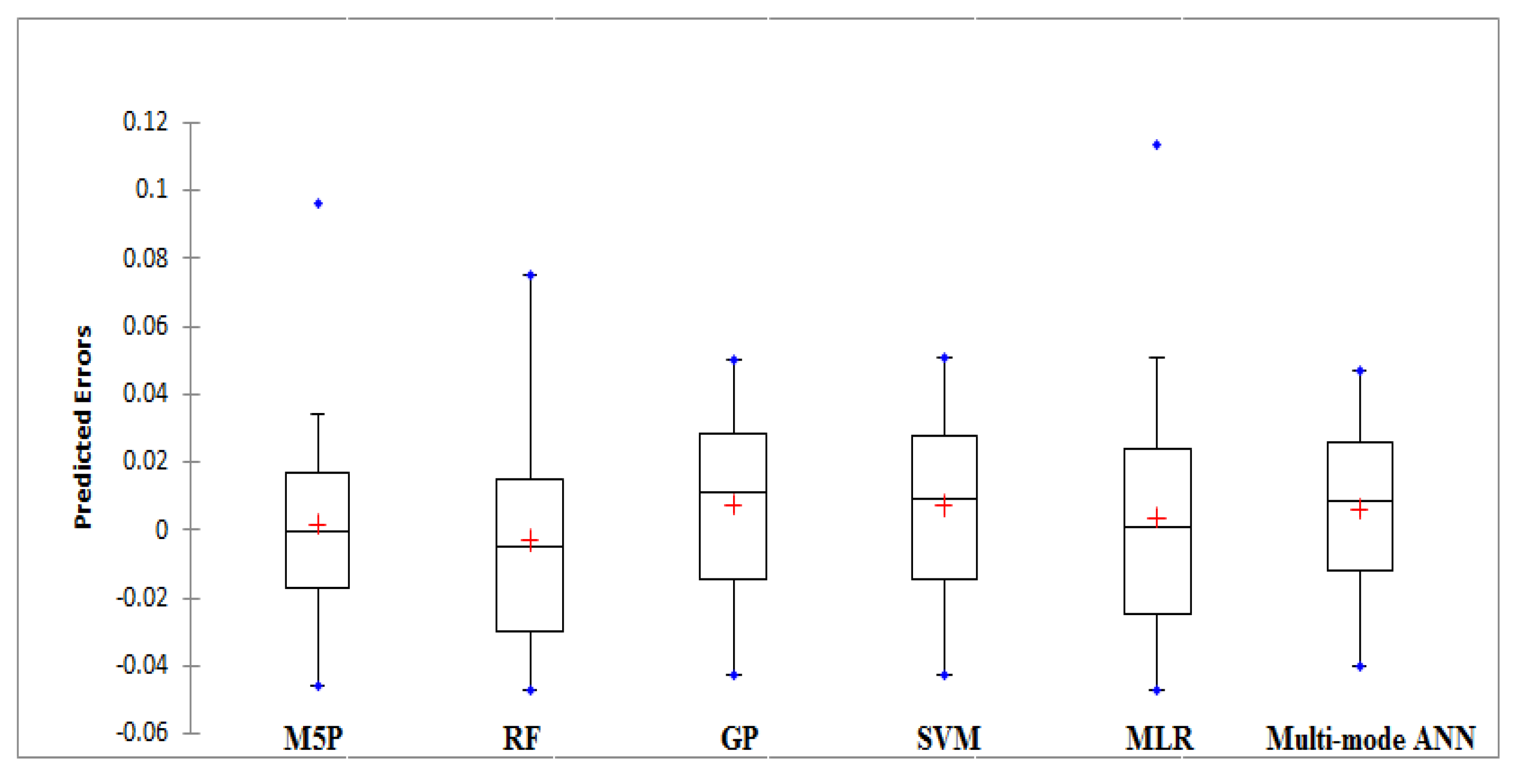
The entire error distribution was plotted using a box plot to evaluate the outcomes (Figure 10). The positive and negative error values indicated the under- and over-prediction tendencies of the models.

Table 8. The statistics of the error distribution of the implemented models during testing.

Statistic	M5P	RF	GP	SVM	MLR	Novel Multimode ANN
Minimum	−0.0460	−0.0470	−0.0420	−0.0420	−0.0468	−0.0400
Maximum	0.0960	0.0750	0.0500	0.0510	0.1130	0.0470
First Quartile	−0.0170	−0.0295	−0.0140	−0.0140	−0.0242	−0.0118
Median	−0.0005	−0.0045	0.0110	0.0095	0.0008	0.0090
Third Quartile	0.0170	0.0153	0.0285	0.0278	0.0242	0.0263
Mean	0.0016	−0.0029	0.0076	0.0073	0.0037	0.0065

lists the distribution of the overall error. The minimum errors, first quartile, median, third quartile and maximum error are also provided in Table 8 and plotted in Figure 10 for all implemented models. The lower quartile value in the multimode ANN model was −0.0118, which was lower than the other considered models. Figure 10 and Table 8 indicated that the maximum and minimum errors predicted by the multimode ANN model were −0.0400 and 0.0470, respectively, which verify the capability of this model in predicting the C_dt of a BCW gate.

Taylor’s diagram [87] in Figure 11 shows the performance of all the developed models in predicting C_dt. Three statistical parameters involving RMSE, CC and standard deviation were used to evaluate the applied models’ accuracy in the Taylor diagram. Figure 11 indicates that the multimode ANN model attained a higher CC with minimal RMSE. The Taylor diagram also confirmed that the performance of the multimode ANN model surpassed the other applied models.

6. Conclusions

Broad-crested weirs are widely used as flood control reservoirs and as measuring structures. Upstream sediment accumulation reduces the performance of broad-crested weirs and similar structures. The combined weir-gate devices can minimize sediment and prevent upstream accumulation [88]. The current study determined the discharge coefficient (C_dt) of a combined compound rectangular broad-crested weir (BCW) gate. For this purpose, the experimental results of a simple broad-crested weir were employed for the code’s calibration, and the k-w model was selected for numerical simulation. The effective parameters of the combined structure were changed for a comprehensive investigation. The studied dimensionless parameters were: b/Bo, d/P, B/Bo, Z/P and h₁/H. A total of 61 compound BCW gates were numerically simulated using different values of the dimensionless parameters. Finally, the results of the calibrated CFD code were used to develop models for the prediction of a compound BCW-gate C_dt. Six data-driven algorithms, including M5P tree, RF, Gaussian process, SVM, MLR and multimode ANN, were used.

The results showed better performance from the SVM model than the RF, M5P, GP and MLR models, in terms of CC, NSE, MAE, RMSE and SI. The sensitivity investigation indicated h₁/H as the most effective parameter, followed by d/p, b/B₀, B/B₀ and z/p, in predicting C_dt using SVM. The novel multimode ANN model outperformed all other models. It reduced the RMSE by 37, 13, 6.9, 6.5 and 32% of the M5P, RF, GP, SVM and MLR, respectively. The Taylor diagram and box plot also confirmed the novel multimode ANN model as the most suitable model in predicting the C_dt of a BCW gate with minimum errors and maximum correlation.

References

1. Salmasi, F.; Nouri, M.; Sihag, P.; Abraham, J. Application of SVM, ANN, GRNN, RF, GP and RT models for predicting discharge coefficients of oblique sluice gates using experimental data. Water Supply 2020, 21, 232–248. [Google Scholar] [CrossRef]
2. Salmasi, F.; Nouri, M.; Abraham, J. Laboratory Study of the Effect of Sills on Radial Gate Discharge Coefficient. KSCE J. Civ. Eng. 2019, 23, 2117–2125. [Google Scholar] [CrossRef]
3. Abbaspour, A.; Yasi, M. Flow over Truncated-Triangular Weirs. Master’s Thesis, University of Urmia, Urmia, Iran, 2001. (In Persian). [Google Scholar]
4. Das, B.S.; Devi, K.; Khatua, K.K. Prediction of discharge in converging and diverging compound channel by gene expression programming. ISH J. Hydraul. Eng. 2019, 27, 385–395. [Google Scholar] [CrossRef]
5. Bos, M.G. Discharge Measurement Structures; International Institute for Land Reclamation and Improvement (ILRI): Wageningen, The Netherlands, 1986. [Google Scholar]
6. Dayev, Z.; Kairakbaev, A.; Yetilmezsoy, K.; Bahramian, M.; Sihag, P.; Kıyan, E. Approximation of the discharge coefficient of differential pressure flowmeters using different soft computing strategies. Flow Meas. Instrum. 2021, 79, 101913. [Google Scholar] [CrossRef]
7. Al-Khatib, I.A.; Gogus, M. Prediction models for discharge estimation in rectangular compound broad-crested weirs. Flow Meas. Instrum. 2014, 36, 1–8. [Google Scholar] [CrossRef]
8. The United States Bureau of Reclamation (USBR). Water Measurement Manual, Chapter 7—Weirs,13, Special Weirs; Retrieved on 10 December 2013. Available online: http://www.usbr.gov/pmts/hydraulics_lab/pubs/wmm/chap07_13.html (accessed on 10 December 2013).
9. Cigno, E.; Magagnoli, C.; Pierce, M.; Iglesias, P. Lubricating ability of two phosphonium-based ionic liquids as additives of a bio-oil for use in wind turbines gearboxes. Wear 2017, 376–377, 756–765. [Google Scholar] [CrossRef]
10. Xu, T.; Jin, Y.-C. Numerical Study of the Flow over Broad-Crested Weirs by a Mesh-Free Method. J. Irrig. Drain. Eng. 2017, 143, 04017034. [Google Scholar] [CrossRef]
11. Göğüş, M.; Defne, Z.; Özkandemir, V. Broad-Crested Weirs with Rectangular Compound Cross Sections. J. Irrig. Drain. Eng. 2006, 132, 272–280. [Google Scholar] [CrossRef]
12. Salmasi, F.; Yıldırım, G.; Masoodi, A.; Parsamehr, P. Predicting discharge coefficient of compound broad-crested weir by using genetic programming (GP) and artificial neural network (ANN) techniques. Arab. J. Geosci. 2012, 6, 2709–2717. [Google Scholar] [CrossRef]
13. Haddadi, H.; Rahimpour, M. A discharge coefficient for a trapezoidal broad-crested side weir in subcritical flow. Flow Meas. Instrum. 2012, 26, 63–67. [Google Scholar] [CrossRef]
14. Altan-Sakarya, A.B.; Kökpınar, M.A. Computation of discharge for simultaneous flow over weirs and below gates (H-weirs). Flow Meas. Instrum. 2013, 29, 32–38. [Google Scholar] [CrossRef]
15. Negm, A.-A.M.; Al-Brahim, A.; Alhamid, A. Combined-free flow over weirs and below gates. J. Hydraul. Res. 2002, 40, 359–365. [Google Scholar] [CrossRef]
16. Alhamid, A.A. Analysis and formulation of flow through combined V-notch-gate-device. J. Hydraul. Res. 1999, 37, 697–705. [Google Scholar] [CrossRef]
17. Samani, J.M.; Mazaheri, M. Combined Flow over Weir and under Gate. J. Hydraul. Eng. 2009, 135, 224–227. [Google Scholar] [CrossRef]
18. Alhamid, A.A.; Husain, D.; Negm, A.A.M. Discharge equation for simultaneous flow over rectangular weirs and below inverted triangular weirs. Arab. Gulf J. Sci. Res. 1996, 14, 595–607. [Google Scholar]
19. Ferro, V. Simultaneous flow over and under a gate. J. Irrig. Drain. Eng. 2000, 126, 190–193. [Google Scholar] [CrossRef]
20. Kisi, O.; Shiri, J.; Karimi, S.; Adnan, R.M. Three Different Adaptive Neuro Fuzzy Computing Techniques for Forecasting Long-Period Daily Streamflows. In Big Data in Engineering Applications; Springer: Singapore, 2018; Volume 44, pp. 303–321. [Google Scholar] [CrossRef]
21. Alizamir, M.; Kisi, O.; Adnan, R.M.; Kuriqi, A. Modelling reference evapotranspiration by combining neuro-fuzzy and evolu-tionary strategies. Acta Geophys. 2020, 68, 1113–1126. [Google Scholar] [CrossRef]
22. Roushangar, K.; Akhgar, S.; Salmasi, F. Estimating discharge coefficient of stepped spillways under nappe and skimming flow regime using data driven approaches. Flow Meas. Instrum. 2018, 59, 79–87. [Google Scholar] [CrossRef]
23. Adnan, R.; Jaafari, A.; Mohanavelu, A.; Kisi, O.; Elbeltagi, A. Novel Ensemble Forecasting of Streamflow Using Locally Weighted Learning Algorithm. Sustainability 2021, 13, 5877. [Google Scholar] [CrossRef]
24. Akbari, M.; Salmasi, F.; Arvanaghi, H.; Karbasi, M.; Farsadizadeh, D. Application of Gaussian Process Regression Model to Predict Discharge Coefficient of Gated Piano Key Weir. Water Resour. Manag. 2019, 33, 3929–3947. [Google Scholar] [CrossRef]
25. Seyedzadeh, A.; Maroufpoor, S.; Maroufpoor, E.; Shiri, J.; Bozorg-Haddad, O.; Gavazi, F. Artificial intelligence approach to estimate discharge of drip tape irrigation based on temperature and pressure. Agric. Water Manag. 2019, 228, 105905. [Google Scholar] [CrossRef]
26. Bahrami, B.; Mohsenpour, S.; Noghabi, H.R.S.; Hemmati, N.; Tabzar, A. Estimation of flow rates of individual phases in an oil-gas-water multiphase flow system using neural network approach and pressure signal analysis. Flow Meas. Instrum. 2019, 66, 28–36. [Google Scholar] [CrossRef]
27. Jahanpanah, E.; Khosravinia, P.; Sanikhani, H.; Kisi, O. Estimation of discharge with free overfall in rectangular channel using artificial intelligence models. Flow Meas. Instrum. 2019, 67, 118–130. [Google Scholar] [CrossRef]
28. Aghaee, A.; Aghaee, M.; Fathi, M.R.; Shoa’Bin, S.; Sobhani, S.M. A novel fuzzy hybrid multi-criteria decision-making approach for evaluating maintenance strategies in petrochemical industry. J. Qual. Maint. Eng. 2020, 27, 351–365. [Google Scholar] [CrossRef]
29. Safari, H.; Etezadi, S.; Moghadam, M.M.; Fathi, M.R. Maturity evaluation of supply chain procedures by combining SCOR and PST models. Int. J. Process Manag. Benchmarking 2021, 11, 707. [Google Scholar] [CrossRef]
30. Maroufpoor, S.; Maroufpoor, E.; Bozorg-Haddad, O.; Shiri, J.; Yaseen, Z.M. Soil moisture simulation using hybrid artificial intelligent model: Hybridization of adaptive neuro fuzzy inference system with grey wolf optimizer algorithm. J. Hydrol. 2019, 575, 544–556. [Google Scholar] [CrossRef]
31. Brandhorst, N.; Erdal, D.; Neuweiler, I. Soil moisture prediction with the ensemble Kalman filter: Handling uncertainty of soil hydraulic parameters. Adv. Water Resour. 2017, 110, 360–370. [Google Scholar] [CrossRef]
32. Salmasi, F.; Sattari, M.T. Predicting Discharge Coefficient of Rectangular Broad-Crested Gabion Weir Using M5 Tree Model. Iran. J. Sci. Technol. Trans. Civ. Eng. 2017, 41, 205–212. [Google Scholar] [CrossRef]
33. Salmasi, F.; Abraham, J. Discharge coefficients for ogee weirs including the effects of a sloping upstream face. Water Supply 2020, 20, 1493–1508. [Google Scholar] [CrossRef]
34. Wang, F.; Zheng, S.; Ren, Y.; Liu, W.; Wu, C. Application of hybrid neural network in discharge coefficient prediction of triangular labyrinth weir. Flow Meas. Instrum. 2021, 83, 102108. [Google Scholar] [CrossRef]
35. Haghiabi, A.H.; Parsaie, A.; Ememgholizadeh, S. Prediction of discharge coefficient of triangular labyrinth weirs using Adaptive Neuro Fuzzy Inference System. Alex. Eng. J. 2018, 57, 1773–1782. [Google Scholar] [CrossRef]
36. Karami, H.; Karimi, S.; Rahmanimanesh, M.; Farzin, S. Predicting discharge coefficient of triangular labyrinth weir using Support Vector Regression, Support Vector Regression-firefly, Response Surface Methodology and Principal Component Analysis. Flow Meas. Instrum. 2017, 55, 75–81. [Google Scholar] [CrossRef]
37. Zaji, A.H.; Bonakdari, H.; Shamshirband, S. Support vector regression for modified oblique side weirs discharge coefficient prediction. Flow Meas. Instrum. 2016, 51, 1–7. [Google Scholar] [CrossRef]
38. Kisi, O.; Emiroglu, M.E.; Bilhan, O.; Guven, A. Prediction of lateral outflow over triangular labyrinth side weirs under subcritical conditions using soft computing approaches. Expert Syst. Appl. 2012, 39, 3454–3460. [Google Scholar] [CrossRef]
39. Emiroglu, M.E.; Bilhan, O.; Kisi, O. Neural networks for estimation of discharge capacity of triangular labyrinth side-weir located on a straight channel. Expert Syst. Appl. 2011, 38, 867–874. [Google Scholar] [CrossRef]
40. Dursun, O.F.; Kaya, N.; Firat, M. Estimating discharge coefficient of semi-elliptical side weir using ANFIS. J. Hydrol. 2012, 426–427, 55–62. [Google Scholar] [CrossRef]
41. Kumar, M.; Sihag, P.; Tiwari, N.K.; Ranjan, S. Experimental study and modelling discharge coefficient of trapezoidal and rectangular piano key weirs. Appl. Water Sci. 2020, 10, 43. [Google Scholar] [CrossRef] [Green Version]
42. Azimi, H.; Bonakdari, H.; Ebtehaj, I. Design of radial basis function-based support vector regression in predicting the discharge coefficient of a side weir in a trapezoidal channel. Appl. Water Sci. 2019, 9, 78. [Google Scholar] [CrossRef] [Green Version]
43. Norouzi, R.; Daneshfaraz, R.; Ghaderi, A. Investigation of discharge coefficient of trapezoidal labyrinth weirs using artificial neural networks and support vector machines. Appl. Water Sci. 2019, 9, 1–10. [Google Scholar] [CrossRef]
44. Bilhan, O.; Emiroglu, M.E.; Miller, C.J.; Ulas, M. The evaluation of the effect of nappe breakers on the discharge capacity of trapezoidal labyrinth weirs by ELM and SVR approaches. Flow Meas. Instrum. 2018, 64, 71–82. [Google Scholar] [CrossRef]
45. Roushangar, K.; Khoshkanar, R.; Shiri, J. Predicting trapezoidal and rectangular side weirs discharge coefficient using machine learning methods. ISH J. Hydraul. Eng. 2016, 22, 254–261. [Google Scholar] [CrossRef]
46. Emiroglu, M.E.; Kisi, O. Prediction of Discharge Coefficient for Trapezoidal Labyrinth Side Weir Using a Neuro-Fuzzy Approach. Water Resour. Manag. 2013, 27, 1473–1488. [Google Scholar] [CrossRef]
47. Haghbin, M.; Sharafati, A. A review of studies on estimating the discharge coefficient of flow control structures based on the soft computing models. Flow Meas. Instrum. 2022, 83, 102119. [Google Scholar] [CrossRef]
48. Zarei, S.; Yosefvand, F.; Shabanlou, S. Discharge coefficient of side weirs on converging channels using extreme learning machine modeling method. Measurement 2019, 152, 107321. [Google Scholar] [CrossRef]
49. Bonakdari, H.; Zaji, A.H. New type side weir discharge coefficient simulation using three novel hybrid adaptive neuro-fuzzy inference systems. Appl. Water Sci. 2018, 8, 10. [Google Scholar] [CrossRef] [Green Version]
50. Ebtehaj, I.; Bonakdari, H.; Gharabaghi, B. Development of more accurate discharge coefficient prediction equations for rectangular side weirs using adaptive neuro-fuzzy inference system and generalized group method of data handling. Measurement 2018, 116, 473–482. [Google Scholar] [CrossRef]
51. Khoshbin, F.; Bonakdari, H.; Ashraf Talesh, S.H.; Ebtehaj, I.; Zaji, A.H.; Azimi, H. Adaptive neuro-fuzzy inference system multi-objective optimization using the genetic algorithm/singular value decomposition method for modelling the dis-charge coefficient in rectangular sharp-crested side weirs. Eng. Optim. 2016, 48, 933–948. [Google Scholar] [CrossRef]
52. Ebtehaj, I.; Bonakdari, H.; Zaji, A.H.; Azimi, H.; Sharifi, A. Gene expression programming to predict the discharge coefficient in rectangular side weirs. Appl. Soft Comput. 2015, 35, 618–628. [Google Scholar] [CrossRef]
53. Aydin, M.C.; Emiroglu, M.E. Determination of capacity of labyrinth side weir by CFD. Flow Meas. Instrum. 2013, 29, 1–8. [Google Scholar] [CrossRef]
54. Ahmad, F.; Hussain, A.; Ansari, M.A. Development of ANN model for the prediction of discharge coefficient of an arced labyrinth side weir. Model. Earth Syst. Environ. 2022, 1–8. [Google Scholar] [CrossRef]
55. Hameed, M.M.; AlOmar, M.K.; Khaleel, F.; Al-Ansari, N. An Extra Tree Regression Model for Discharge Coefficient Prediction: Novel, Practical Applications in the Hydraulic Sector and Future Research Directions. Math. Probl. Eng. 2021, 2021, 1–19. [Google Scholar] [CrossRef]
56. Jamei, M.; Ahmadianfar, I.; Chu, X.; Yaseen, Z.M. Estimation of triangular side orifice discharge coefficient under a free flow condition using data-driven models. Flow Meas. Instrum. 2020, 77, 101878. [Google Scholar] [CrossRef]
57. Gharib, R.; Heydari, M.; Kardar, S.; Shabanlou, S. Simulation of discharge coefficient of side weirs placed on con-vergent canals using modern self-adaptive extreme learning machine. Appl. Water Sci. 2020, 10, 50. [Google Scholar] [CrossRef] [Green Version]
58. Mehri, Y.; Soltani, J.; Khashehchi, M. Predicting the coefficient of discharge for piano key side weirs using GMDH and DGMDH techniques. Flow Meas. Instrum. 2018, 65, 1–6. [Google Scholar] [CrossRef]
59. Zaji, A.H.; Bonakdari, H.; Khodashenas, S.R.; Shamshirband, S. Firefly optimization algorithm effect on support vector regression prediction improvement of a modified labyrinth side weir’s discharge coefficient. Appl. Math. Comput. 2016, 274, 14–19. [Google Scholar] [CrossRef]
60. Göğüş, M.; Al-Khatib, I. Flow-Measurement Flumes of Rectangular Compound Cross Section. J. Irrig. Drain. Eng. 1995, 121, 135–142. [Google Scholar] [CrossRef]
61. Ozkandemir, V. Hydraulic Characteristics of Broad-Crested Weirs of Rectangular Compound Cross-Section. Master’s Thesis, Middle East Technical University, Ankara, Turkey, 1997. [Google Scholar]
62. Henry, H.R. Discussion of diffusion of submerged jets by ML Albertson, YBDai, RA Jensen, H Rouse. Trans. ASCE 1950, 115, 687–694. [Google Scholar]
63. Safarzadeh, A.; Mohajeri, H. Hydrodynamics of rectangular broad crested porous weirs. J. Irrig. Drain. Eng. 2018, 144, 8–24. [Google Scholar] [CrossRef]
64. Hirt, C.; Nichols, B. Volume of fluid (VOF) method for the dynamics of free boundaries. J. Comput. Phys. 1981, 39, 201e225. [Google Scholar] [CrossRef]
65. Rashid, M.A.; Abustan, I.; Hamzah, M.O. Numerical simulation of a 3-D flow within a storage areahexagonal modular pavement systems. In Proceedings of the 4th International Conference on Energy and Environment 2013 (ICEE 2013), Putrajaya, Malaysia, 20–22 December 2013. [Google Scholar] [CrossRef] [Green Version]
66. Parsaie, A.; Haghyabi, A.; Moradinejad, A. CFD modeling of flow pattern in spillway’s approach channel. Water Resour. Manag. 2015, 1, 245–251. [Google Scholar] [CrossRef] [Green Version]
67. Bayon, A.; Valero, D.; Bartual, R.G.; Valles Moran, F.J.; Jimenez, P.A.L. Performance assessment of Open FOAM and FLOW-3D in the numerical modeling of a low Reynolds number hydraulic jump. Environ. Model. Softw. 2016, 80, 322–335. [Google Scholar] [CrossRef]
68. Hirt, C.W.; Sicilian, J.M. A porosity technique for the definition of obstacles in rectangular cell meshes. In Proceedings of the 4th International Conference on Ship Hydro dynamics, Washington, DC, USA, 24–27 September 1985; National Academy of Sciences: Washington, DC, USA, 1985. [Google Scholar]
69. Behbahani, S.D.; Parsaie, A. Numerical modeling of flow pattern in dam spillway’s guide wall. Case study: Balaroud dam, Iran. Alexandria Eng. J. 2016, 55, 467–473. [Google Scholar] [CrossRef] [Green Version]
70. Abbaspoor, A.; Yasi, M. Investigation of Flow in Combined Rectangular-Triangular Weir. Ph.D. Thesis, Urmia University, Urmia, Iran, 2002. [Google Scholar]
71. Yakhot, V.; Orszag, S.A. Re normalization Group Analysis of Turbulence: Basic Theory. J. Sci. Comput. 1986, 1, 3–51. [Google Scholar] [CrossRef]
72. Cable, M. An Evaluation of Turbulence Models for the Numerical Study of Forced and Natural Convective Flow in Atria. Ph.D. Thesis, Queens University, Kingston, ON, Canada, 2009. [Google Scholar]
73. Wilcox, D.C. Turbulence Modeling for CFD; DCW Industries Inc.: La Canada, CA, USA, 1998. [Google Scholar]
74. Quinlan, J.R. Learning with continuous classes. In Proceedings of the 5th Australian Joint Conference on Artificial Intelligence, Hobart, Tasmania, 16–18 November 1992; Volume 92, pp. 343–348. [Google Scholar]
75. Solomatine, D.P.; Xue, Y. M5 Model Trees and Neural Networks: Application to Flood Forecasting in the Upper Reach of the Huai River in China. J. Hydrol. Eng. 2004, 9, 491–501. [Google Scholar] [CrossRef]
76. Jothiprakash, V.; Kote, A.S. Effect of Pruning and Smoothing while Using M5 Model Tree Technique for Reservoir Inflow Prediction. J. Hydrol. Eng. 2011, 16, 563–574. [Google Scholar] [CrossRef]
77. Breiman, L. Bagging predictors. Mach. Learn. 1996, 24, 123–140. [Google Scholar] [CrossRef] [Green Version]
78. Breiman, L. Random forests. Mach. Learn. 2001, 45, 5–32. [Google Scholar] [CrossRef] [Green Version]
79. Liu, H.; Ong, Y.-S.; Shen, X.; Cai, J. When Gaussian Process Meets Big Data: A Review of Scalable GPs. IEEE Trans. Neural Netw. Learn. Syst. 2020, 31, 4405–4423. [Google Scholar] [CrossRef] [Green Version]
80. Pasolli, L.; Melgani, F.; Blanzieri, E. Gaussian process regression for estimating chlorophyll concentration in sub-surface waters from remote sensing data. IEEE Geosci. Remote Sens. Lett. 2010, 7, 464–468. [Google Scholar] [CrossRef]
81. Sihag, P.; Tiwari, N.K.; Ranjan, S. Modelling of infiltration of sandy soil using gaussian process regression. Model. Earth Syst. Environ. 2017, 3, 1091–1100. [Google Scholar] [CrossRef]
82. Shabani, S.; Samadianfard, S.; Sattari, M.T.; Mosavi, A.; Shamshirband, S.; Kmet, T.; Várkonyi-Kóczy, A.R. Modeling Pan Evaporation Using Gaussian Process Regression K-Nearest Neighbors Random Forest and Support Vector Machines; Comparative Analysis. Atmosphere 2020, 11, 66. [Google Scholar] [CrossRef] [Green Version]
83. Yu, Y.; Li, Y.; Li, J. Forecasting hysteresis behaviors of magnetorheological elastomer base isolator utilizing a hybrid model based on support vector regression and improved particle swarm optimization. Smart Mater. Struct. 2015, 24, 035025. [Google Scholar] [CrossRef]
84. Yu, Y.; Li, Y.; Li, J.; Gu, X. Self-adaptive step fruit fly algorithm optimized support vector regression model for dynamic response prediction of magnetorheological elastomer base isolator. Neurocomputing 2016, 211, 41–52. [Google Scholar] [CrossRef] [Green Version]
85. Sihag, P.; Jain, P.; Kumar, M. Modelling of impact of water quality on recharging rate of storm water filter system using various kernel function based regression. Model. Earth Syst. Environ. 2018, 4, 61–68. [Google Scholar] [CrossRef]
86. Haykin, S. Self-Organizing Maps. Neural networks—A Comprehensive Foundation, 2nd ed.; Prentice-Hall: Hoboken, NJ, USA, 1999. [Google Scholar]
87. Taylor, K.E. Summarizing multiple aspects of model performance in a single diagram. J. Geophys. Res. Atmos. 2001, 106, 7183–7192. [Google Scholar] [CrossRef]
88. Nouri, M.; Hemmati, M. Discharge coefficient in the combined weir-gate structure. Flow Meas. Instrum. 2020, 75, 101780. [Google Scholar] [CrossRef]
Figure 1. (a) Definition sketch of compound BCW: (b,c) two diverse flow cases through the compound BCW segment.
Sustainability 15 00433 g001
Figure 2. (a) Sketch for simultaneous flow over compound BCW and below gate: (b,c) are two diverse flow cases through the combined compound BCW gate.
Sustainability 15 00433 g002aSustainability 15 00433 g002b
Figure 3. Single broad-crested weir studied by Salmasi et al., [12].
Sustainability 15 00433 g003
Figure 4. Estimated Cdw using numerical models; (a) Broad crested weir with B/B0 = 0.24, (b)Broad crested weir with B/B0 = 0.32.
Sustainability 15 00433 g004
Figure 5. Combined compound BCW gate and boundary conditions used; Xmin: P (specified pressure); Xmax: O (outflow); Ymin, Ymax and Zmin: W (wall); Zmax: S (symmetry).
Sustainability 15 00433 g005
Figure 6. Structure of ANN.
Sustainability 15 00433 g006
Figure 7. Performance of M5P, RF, GP, SVM and MLR models in predicting Cdt of BCW gate during model calibration and validation.
Sustainability 15 00433 g007
Figure 8. Structure of the novel multimode ANN model.
Sustainability 15 00433 g008
Figure 9. Agreement plot of multimode ANN prediction with observed Cdt of BCW gate during training and testing.
Sustainability 15 00433 g009
Figure 10. Box plot of the error distribution of the applied models during testing.
Sustainability 15 00433 g010
Figure 11. Taylor diagram for M5P, RF, GP, SVM, MLR and novel multimode ANN models.
Sustainability 15 00433 g011