Crop Type Prediction: A Statistical and Machine Learning Approach

Abstract

Farmers’ ability to accurately anticipate crop type is critical to global food production and sustainable smart cities since timely decisions on imports and exports, based on precise forecasts, are crucial to the country’s food security. In India, agriculture and allied sectors constitute the country’s primary source of revenue. Seventy percent of the country’s rural residents are small or marginal agriculture producers. Cereal crops such as rice, wheat, and other pulses make up the bulk of India’s food supply. Regarding cultivation, climate and soil conditions play a vital role. Information is of utmost need in predicting which crop is best suited given the soil and climate. This paper provides a statistical look at the features and indicates the best crop type on the given features in an Indian smart city context. Machine learning algorithms like k-NN, SVM, RF, and GB trees are examined for crop-type prediction. Building an accurate crop forecast system required high accuracy, and the GB tree technique provided that. It outperforms all the classification algorithms with an accuracy of 99.11% and an F1-score of 99.20%.

1. Introduction

India has the world’s second-largest population, with 1.27 billion people [1]. It has a total landmass of 3.288 million square kilometers, which places it as the sixth largest country on the planet. It has one of the most extensive coastlines in the world, measuring 7500 km in total. In India, people speak over 415 dialects and 22 major languages. India offers a diverse range of agricultural and ecological circumstances due to geographical features such as the Himalayas to the north, the deserts of Thar and the Deccan Plateau to the south, and the Ganges delta to the east. Along with milk, pulses, and jute, India’s other main agricultural exports include rice, wheat, sugarcane, groundnuts, vegetables, fruit, cotton, and a variety of other vegetables and fruits [2,3]. This region is also responsible for plantation crops, spices, fish, poultry, and cattle [4]. With a gross domestic product of USD 2.1 trillion, India is the third biggest economy in the world, behind only the United States and China [5]. Two-thirds of India’s workforce is employed in agriculture, making it the country’s principal sector for job creation [6,7]. As a direct consequence of this primary activity, significant amounts of food grains and raw materials for the industry are generated. Because India is such a large nation, its farmers can cultivate a diverse range of crops [8].

It is essential to the success of global food production and to sustainable smart cities that farmers have the capacity to properly forecast crop type [9,10,11,12]. Choices made promptly about imports and exports, based on accurate estimates, are essential to the nation’s food security. To generate better varieties, breeders need seed producers who can accurately predict how new hybrids will function in various environments. The ability to accurately forecast the type and yield empowers growers and farmers to make more informed decisions on management and finances [13]. However, since so many different factors are involved, it is not easy to accurately forecast agricultural production [14].

The field of artificial intelligence (AI) focuses on learning, and machine learning (ML) is one of the most effective methods to enhance crop prediction by using a wide variety of data [15,16]. Artificial intelligence is a subfield of computing [17]. Using machine learning, it is possible to mine datasets in search of patterns and correlations [18]. To train the models, they need to be given datasets that include information that reflects previous results. During the phase known as ‘training’, past data is used to determine the parameters of the prediction model being constructed utilizing many features. During the ‘testing’ phase, performance is assessed using historical data that was not considered during the training phase [19].

Artificial Intelligence has played a major role in agriculture [14,20,21,22,23,24,25]. Crop yield is one of the major domains where the tools of AI can be molded for estimation of the same [15,26,27,28]. In the area of the type of crop prediction, some articles like [29] deal with the fact that accurate crop type maps are not readily accessible at the beginning of the growing season, and it is not possible to utilize satellite data to construct crop condition and production projections using satellite images alone. This study presents a novel crop-type prediction modeling approach based on deep Neural Networks. The method uses previous crop maps across Nebraska to generate preseason crop-type maps at the field size level.

Ref. [30] is a study conducted in the Brazilian state of Rio Grande do Sul to devise a system for categorizing agricultural products. Rice, soybeans, and maize were the three crops that were used in the creation of the summer crop map layer. The crop classification model has an accuracy rating of 0.95 on the whole. It was shown that the size of the sample, as well as the spatial diversity, affected the performance of the model.

In Ref. [31], a first attempt is made to use machine learning to anticipate annual crop planting using historical crop planting maps. Cropland Data Layer (CDL) time series and a multi-layer artificial neural network were used in this research project as reference data and prediction models, respectively. The proposed structure was piloted for the first time in Lancaster County, Nebraska State, and after its success, it was rolled out to the rest of the Corn Belt. Papers like Ref. [32] deal with an intensive survey of the digital techniques present to predict the crop type. Furthermore, based on farmers’ declaration, crop types were predicted in [33].

For Ref. [34], information that has had its dimensionality reduced is used to generate climate forecasts that have a reasonable possibility of coming true. The classification technique known as Deep Neural Network is used in planning an appropriate growing season for a certain crop. This research endeavor depends on creating a suitable information model to accomplish high accuracy and simplicity in the value prediction process.

In Ref. [35], the authors provide an operational domain adaptation framework for crop type verification using remote sensing data. To train the machine learning model, each variety of the target crop was used. To acquire the metrics, one must first determine the degree to which the vegetation index time series of the observed parcel and the aggregated time series of reference objects are comparable.

Within the scope of Ref. [36], Random Forest models for categorizing crop types in Germany were examined for their capacity to be geographically transferred. Comparing the effects of SAR and optical-SAR data combined on various input datasets was done to find the optimal technique that delivers the most accurate findings in transfer areas. This was accomplished by intensive research into both types of data combinations.

In this research [37], the Grey forecasting technique was adopted to create very accurate prediction data for patterns and trends in crop production from the research findings application of Grey forecasting models for predicting the output of food crops. Incomplete historical data was used with linear equations to accurately calculate patterns and trends in grey forecasting models.

It is seen that the machine learning techniques on geospatial data were focused on other countries except India. Moreover, researchers were concentrating more on crop yield rather than crop selection. In our study, we take the help of an Indian crop dataset integrated with other soil-based and weather-based attributes to classify the crop type. This paper first provides an in-depth statistical analysis of the various attributes of soil like nitrogen, phosphorous, potassium, and pH ratios and various climatic attributes like temperature, humidity, and rainfall which lead to crop selection in a certain geographic area. A feature importance algorithm calculates the most important attribute among them. Finally, the data is fed to machine learning algorithms to model the crop type given the attributes, and we discuss the various performance metrics of those algorithms.

This study first provides the methodologies used in the article in the next section. The results and discussions are provided in Section 3 and Section 4, respectively. Finally, we conclude the article with future scope in Section 5.

2. Methodology

2.1. Dataset Description

A total of 22 crops included in the Food and Agricultural Organisation (FAO) [38], comprising of rice, maize, chickpea, kidney beans, pigeon peas, moth beans, mungbean, black gram, lentil, pomegranate, banana, mango, grapes, watermelon, muskmelon, apple, orange, papaya, coconut, cotton, jute, and coffee, are the main sources of production in India. Along with the crop yield, the dataset contains the following attributes: N—the ratio of Nitrogen content in soil; P—the ratio of Phosphorous content in soil; K—the ratio of Potassium content in soil; temperature—the temperature in degrees Celsius; humidity—relative humidity in %; pH—pH value of the soil; rainfall—rainfall in mm. A total of 35,505 instances are collected from 1961 to 2022.

2.2. Preliminary Statistical Analysis

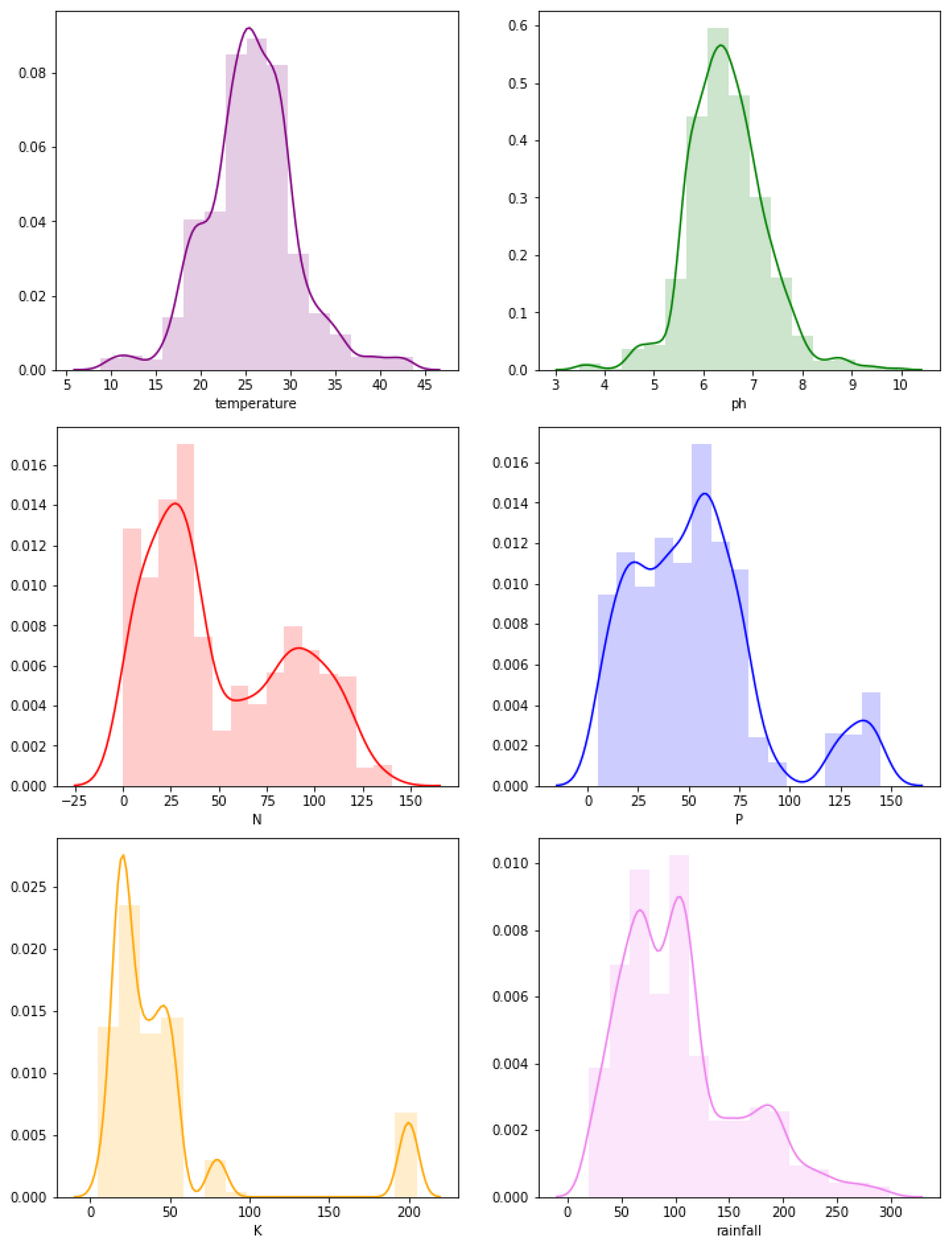
We perform some statistical analysis of the data before implementing machine learning algorithms. The distribution of the attributes is shown in Figure 1. It is seen that temperature and pH value show a similar distribution.

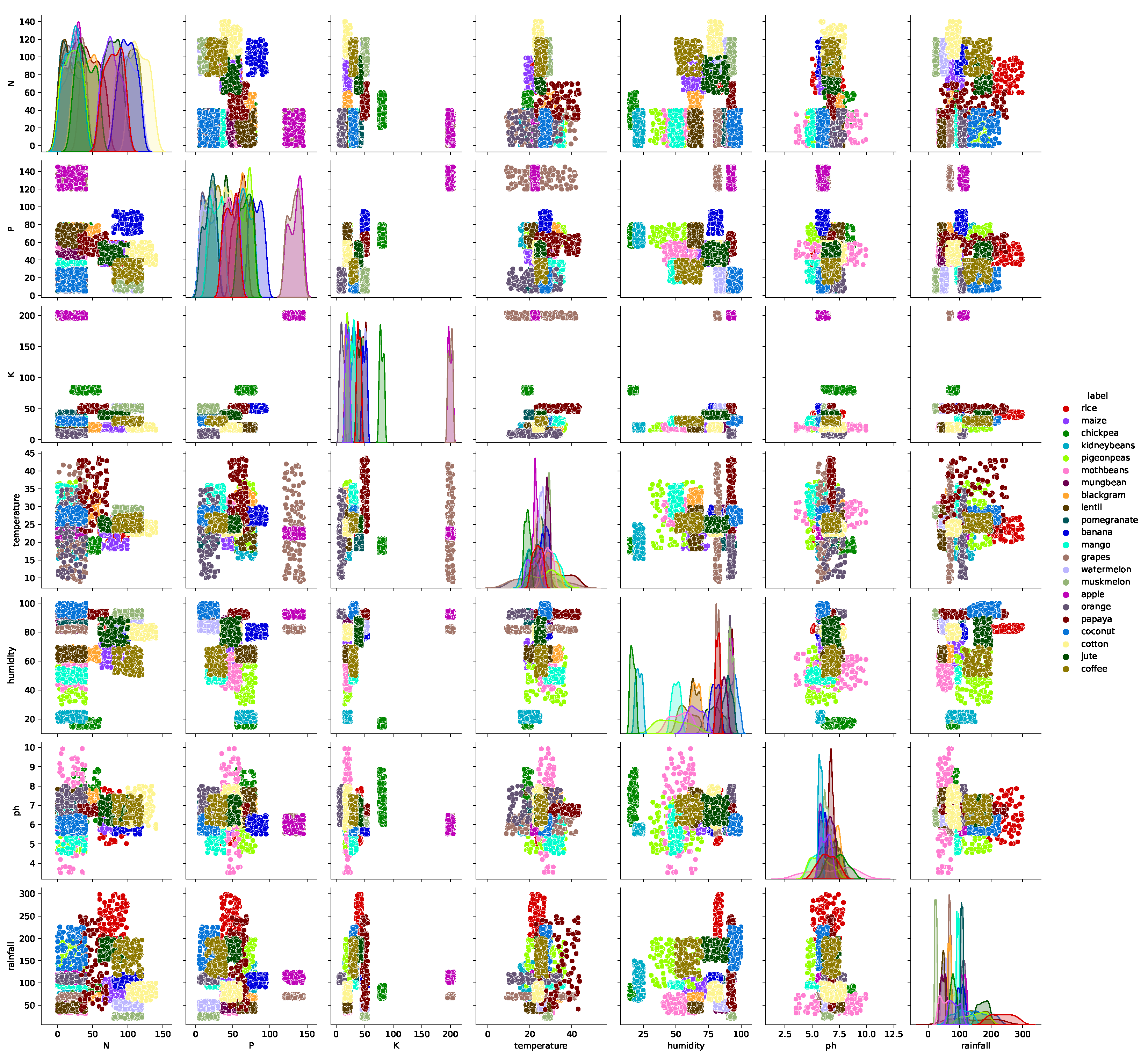
The diagonal distribution of the attributes is shown in Figure 2. A great deal of visual analysis can be inferred from it. For example, the crop ‘rice’ requires heavy rainfall with high relative humidity to survive. ‘Coconuts’, too, require high relative humidity; hence, they are grown and exported from major parts of the coastal regions of India.

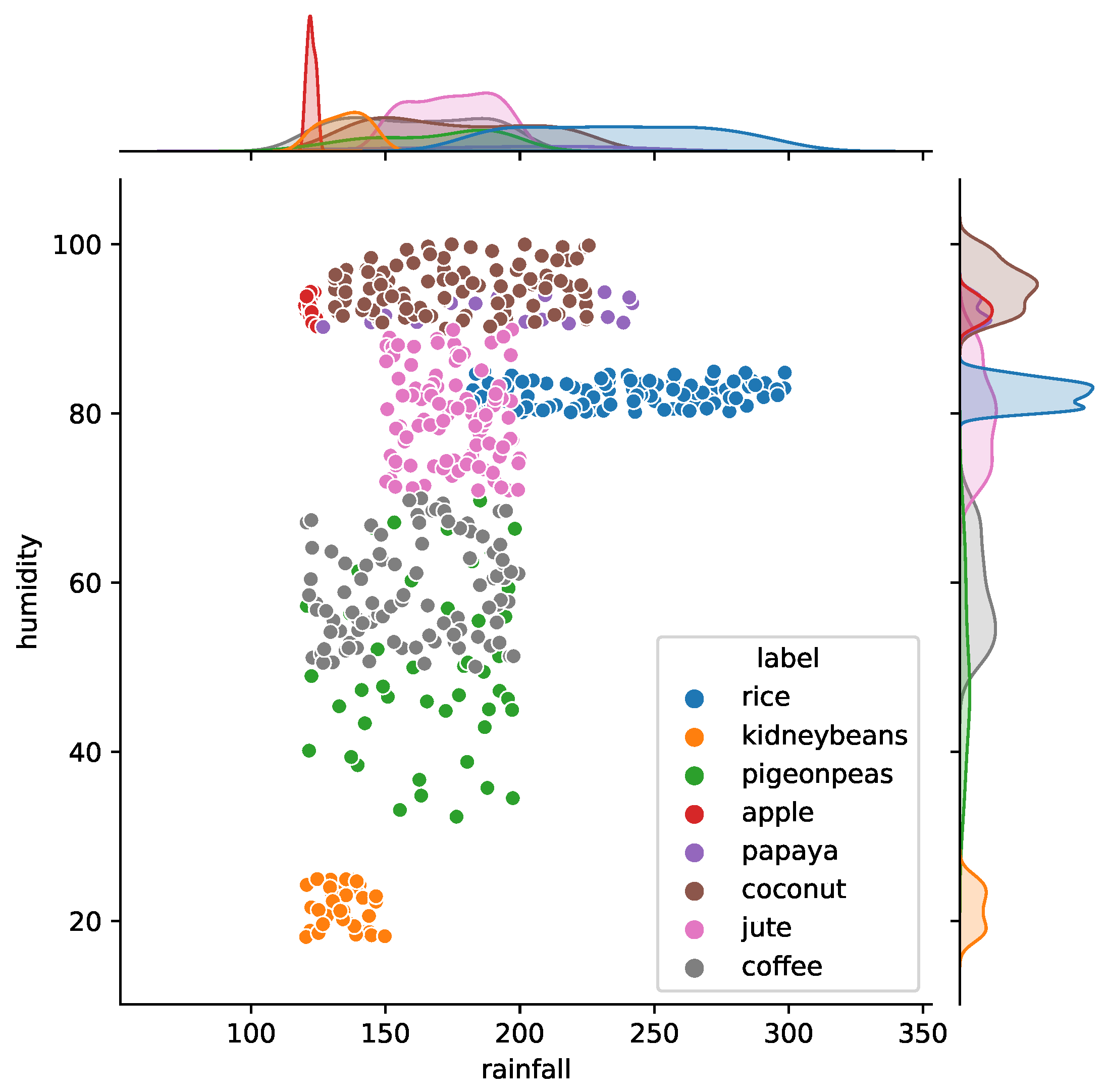
Certain crops require a specific level of humidity and rainfall in India. Figure 3 shows a joint plot between the two factors which impact crop cultivation. For example, rice is cultivated with a relative humidity of 80%, and rainfall ranges from 150 mm to 300 mm. This is a geographical reason why rice is cultivated on the eastern coast of India [39]. Similarly, kidney beans’ relative humidity and rainfall requirements are low compared to rice. The coastal regions of India export coconuts as a major source because the humidity is very high in those regions [40].

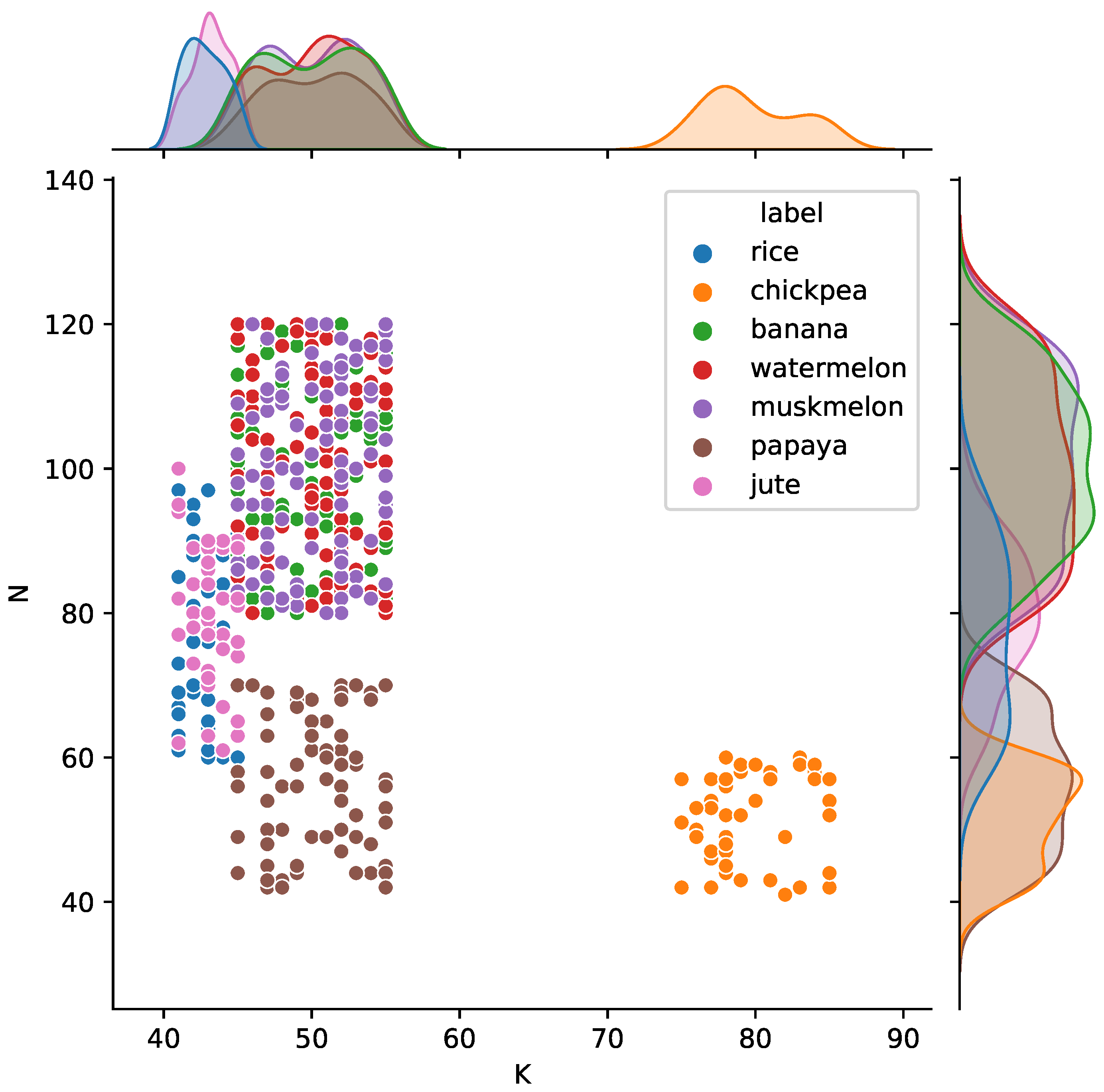
Similarly, crops require a certain ratio of potassium ‘K’ and nitrogen ‘N’ contents in soil. Figure 4 shows a joint plot between the two factors which impact crop cultivation.

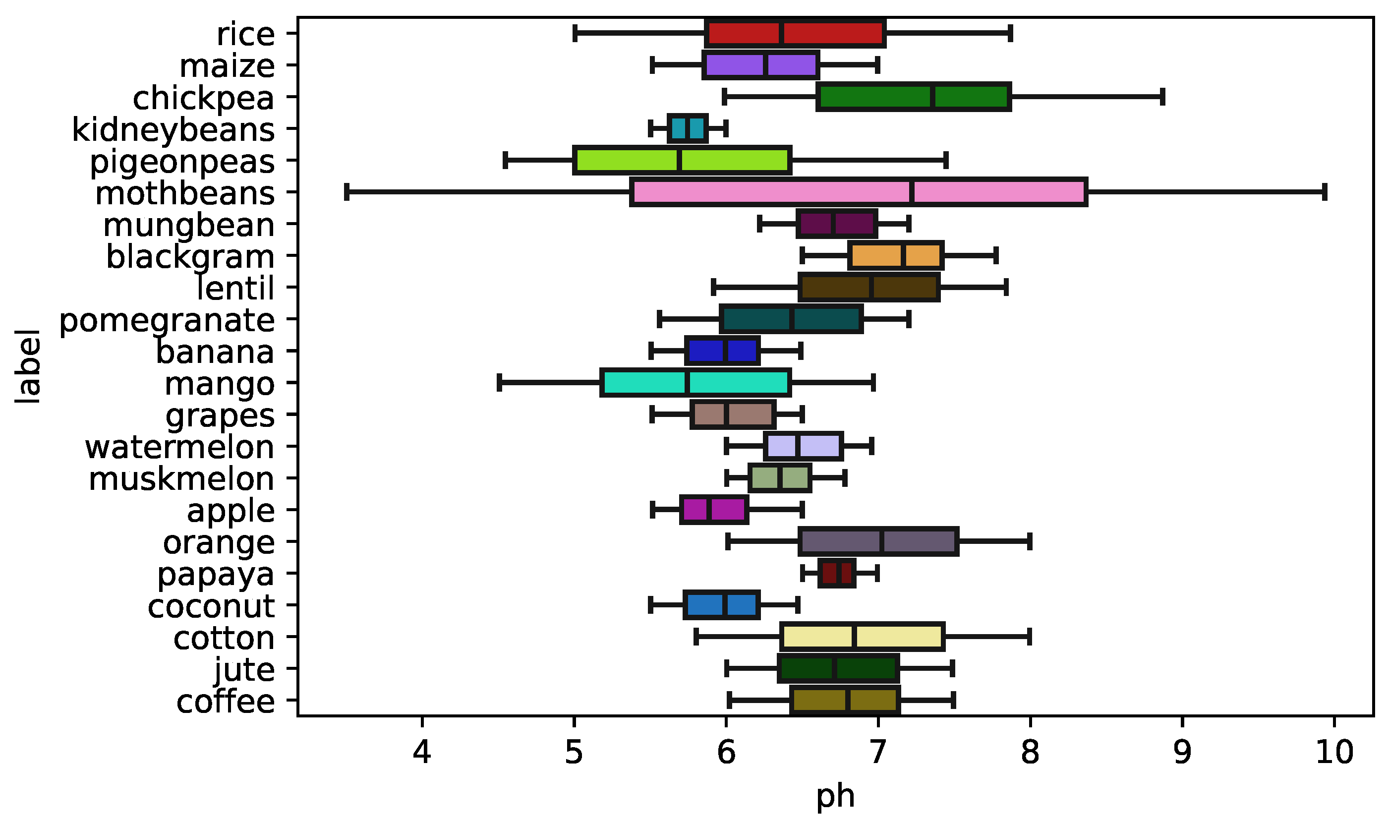
Figure 5 shows the impact of the pH value of the soil as a box plot. For good cultivation, a value between 6 and 7 is recommended.

2.3. Data Pre-Processing

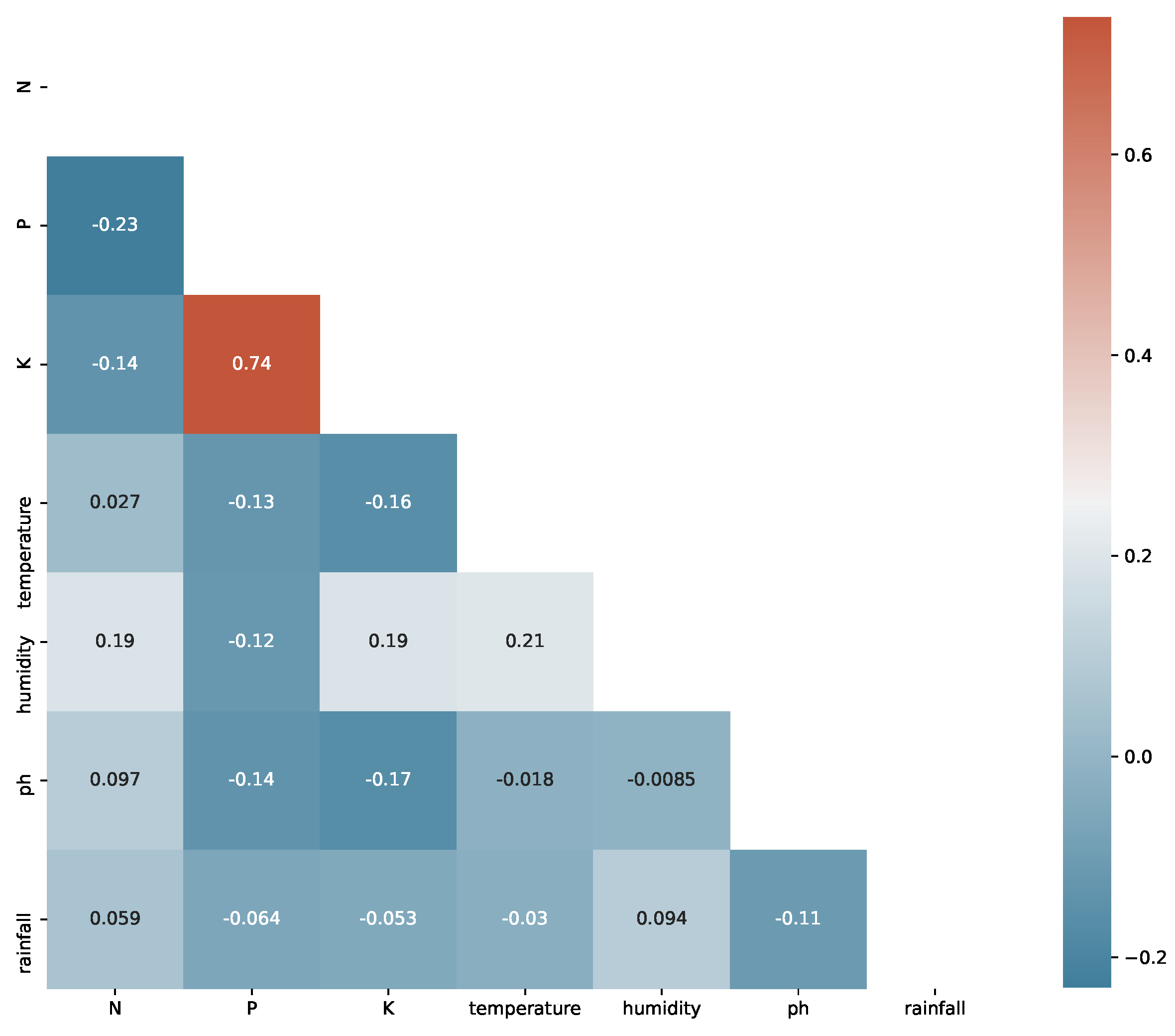
To find dependency between the attributes, this study first uses Pearson’s correlation [41] given as:

$$\rho =\frac{n(\sum {\alpha }_i{\beta }_i)-(\sum {\alpha }_i)(\sum {\beta }_i)}{\sqrt{[n\sum {\alpha }_i^2-{(\sum {\alpha }_i)}^2][n\sum {\beta }_i^2-{(\sum {\beta }_i)}^2]}}$$

(1)

where $\rho$ is the Pearson’s correlation coefficient, n is the total number of instances, ${\alpha }_i$ is the value of each instance i for the attribute $\alpha$ and ${\beta }_i$ is the value of each instance i for the attribute $\beta$. As the value lies within the range of −1 and +1, we can generate a heat map of the same. The heat map matrix for our set of attributes is shown in Figure 6.

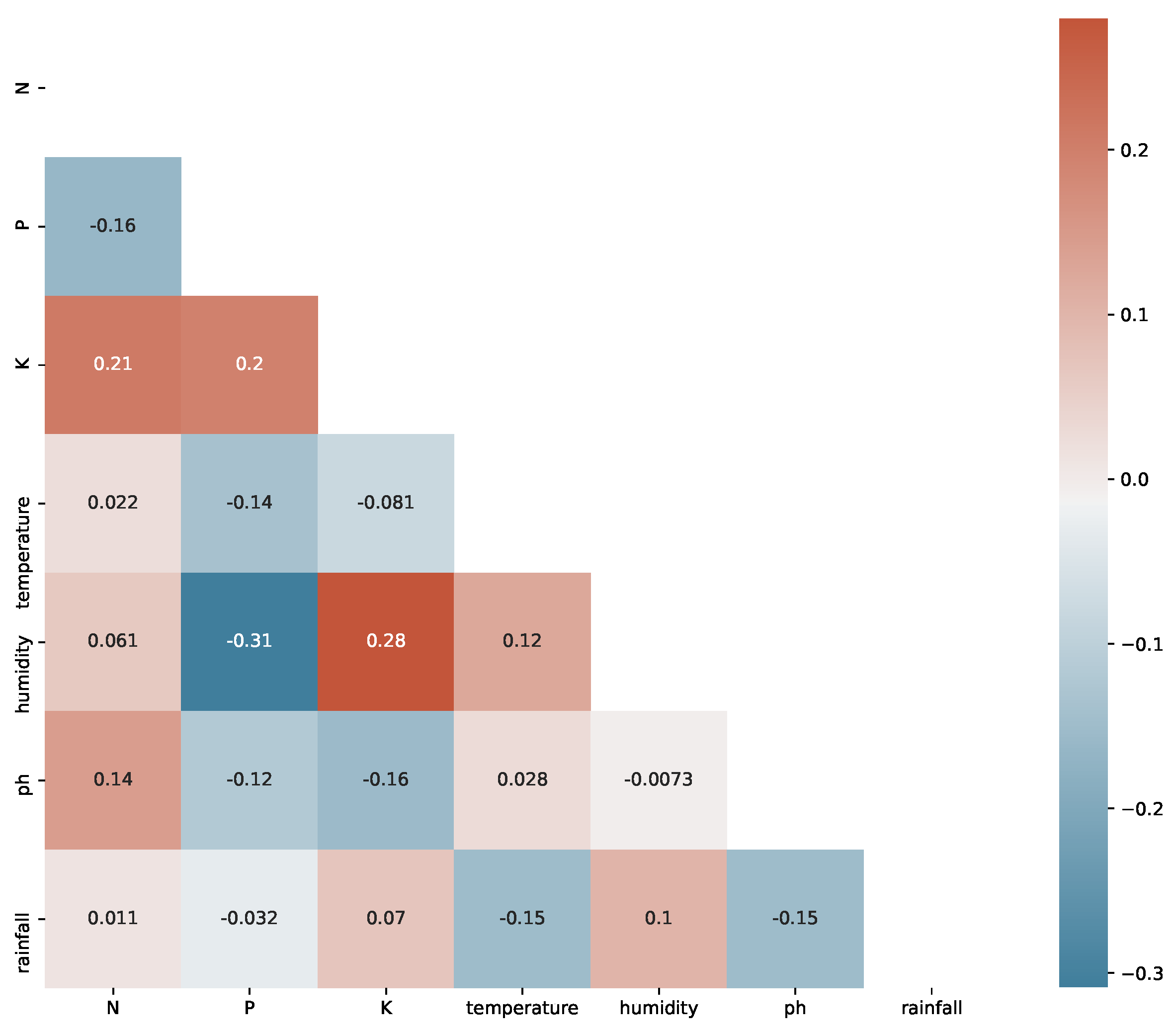
It is already seen in Figure 1 that although ‘temperature’ and ‘pH’ follows the normal distribution; ‘N’, ‘P’, ‘K’, and ‘rainfall’ are far from it. We use Spearman’s correlation coefficient for the attributes which are not normal. The heat map matrix in Figure 7 shows the attributes’ correlations.

Now, we might be able to reduce the impact of outlier data for distributions that are not normal on our model by using the normalization technique. Distance algorithms such as KNN, K-means, and SVM are affected by a large number of different parameters, because comparisons of data points are made based on how closely they are situated to one another. Hence, we use the min–max feature scaling [42] using the following equation:

$${\alpha }_{new}=\frac{\alpha -{\alpha }_{min}}{{\alpha }_{max}-{\alpha }_{min}}$$

(2)

2.4. Classification

2.4.1. k-Nearest Neighbor (k-NN)

If one is searching for a machine learning method that can be used to solve classification and regression challenges, then the k-NN algorithm could be just what one is looking for. K-NN stands for “k-nearest neighbor” [43], an algorithm developed by Evelyn Fix and Joseph Hodges in 1951 and later expanded by Thomas Cover. It creates a decision boundary by assigning the new data to a grouping most closely linked to the existing groupings. This assumes that the new data and the existing instances are similar. We use the distance measure as:

$$D(\alpha ,\beta )=\sqrt{(\sum {({\alpha }_i-{\beta }_i)}^2)}$$

(3)

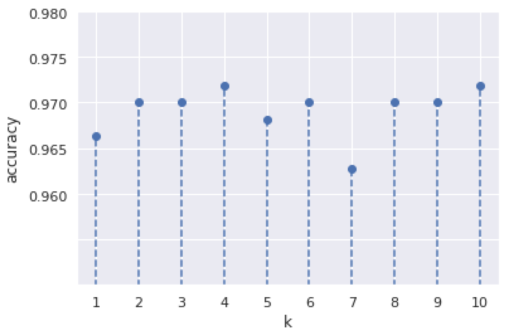
We put each data set through many iterations of the KNN algorithm with a variety of ‘k’ values to identify the importance of it that results in the fewest errors while still allowing the system to accurately predict the outcome of fresh data inputs. This process is repeated for each data set. Figure 8 shows the variation in accuracy for different values of ‘k’ for our study.

2.4.2. Support Vector Machine (SVM)

In the Support Vector Machine (SVM) approach [44], data points are represented by n-dimensional coordinates (where n is the number of features), and a particular value represents each feature in one of those n-dimensional coordinates. The next step in the classification process is choosing the hyperplane that effectively differentiates the two classes. Kernels play a very important role in this part. It is defined as the inner product in the dimensional space. Mathematically,

$$K(\alpha ,\beta )=<\mathsf{\Phi }\left(\alpha \right),\mathsf{\Phi }\left(\beta \right)>$$

(4)

In the event of a particular problem, it could be required to spend a significant amount of time fine-tuning the kernel’s parameters. The data is mapped onto a space with a higher dimension in the hope that it will be simpler to partition or be more efficiently organized in the higher dimensional region.

The phrase “linearly separable” refers to a situation in which it is possible to partition data along a single line, which is when the Linear kernel algorithm is used. When it comes to kernels, this is one of the ones used most often. This is the most typical method, and it comes with several capabilities for summarising enormous volumes of data. Mathematically,

$$K(\alpha ,\beta )={\alpha }^T\beta +c$$

(5)

where ‘c’ is a constant. For non-linear models with a slope of $\Delta$ and degree p, we use the Polynomial kernel defined as:

$$K(\alpha ,\beta )={(\Delta {\alpha }^T\beta +c)}^p$$

(6)

When it comes to the activation of artificial neurons, bipolar sigmoid functions are often used, and the Sigmoid Kernel is based on these functions. In a support vector machine model, two-layer perceptron neural networks may be created using sigmoid kernels. Since it was based on the idea of neural networks, this kernel was a popular option for support vector machines. Formally,

$$K(\alpha ,\beta )=tanh(\Delta {\alpha }^T\beta +c)$$

(7)

Finally, Radial Basis Function (RBF) kernels are one of the most often used forms of kernelization. This is mostly because RBF kernels have a similar appearance to the Gaussian distribution. The RBF kernel function determines how similar two features, denoted by $\alpha$ and $\beta$, are to one another by calculating their proximity with a standard deviation of $\delta$. Mathematically,

$$K(\alpha ,\beta )=exp(-\frac{\left|\right|\alpha -{\beta \left|\right|}^2}{2{\delta }^2})$$

(8)

It is essential to remember that the gamma value is only used in the RBF kernel, and its purpose is to establish how much curvature is required in a decision boundary on a hyperplane in the SVM space.

2.4.3. Decision Tree (DT)

The decision tree algorithm [45] is frequently utilized for classification and regression tasks of supervised machine learning. It categorizes objects based on rules. An attribute selection heuristic may be used to choose splitting criteria for optimal data partitioning. It is called the “splitting rules” because it helps us discover a tuple’s breakpoint. The highest-scoring characteristic will be used to divide. Continuous-valued properties need branch split points. Most selection metrics employ Gini Index and Information Gain.

The entropy of a dataset is a measure of how unpredictable or contaminated it is. This word refers to a lack of purity in an entity while addressing information theory. Information gain is the opposite of entropy in that it quantifies the increase in entropy. Entropy before and after the split is computed based on the supplied characteristics. With $p_i$ being the probability of a data in $\alpha$ in a class $C_j$; we mathematically define it as,

$$Info\left(\alpha \right)=-\sum p_{i}log{p}_i$$

(9)

We use the Gini index, the Gini coefficient, or the Gini impurity to estimate how likely a specific variable will be mistakenly classified randomly. A variable split should have a low Gini Index. Mathematically,

$$Gini\left(\alpha \right)=1-\sum {\left(p_i\right)}^2$$

(10)

2.4.4. Random Forest (RF)

To categorize data, decision trees are used, and a conglomeration of various decision trees is called a random forest [46]. The result is a consequence of the collaborative efforts of all of these trees. The forecasts of each class are determined by a straightforward voting process, with the class that receives the most votes becoming victorious. In this study, the bagging method was used to improve the performance of a single tree for categorization purposes. In training, the number of decision trees was tested with {10, 20, 30, 40, 50, 60, 70, 80, 90, 100, 150, 200, 300, 400, 500} to find the best count in terms of accuracy. It is found that a random forest with 100 decision trees gives the best result in terms of accuracy with the Gini index.

2.4.5. Gradient Boosting (GB)

Gradient-boosted trees are used as an alternative to random forest [47]. In most cases, these trees are the superior performer to random forest [48]. A gradient-boosted trees model is constructed stage-by-stage, much as other boosting algorithms were, but this enables the optimization of any arbitrary differentiable loss function. To put it another way, gradient boosting is a functional gradient iterative approach that minimizes the size of an input value’s loss function by iteratively picking a negative function in the gradient. This is done to improve the accuracy of the prediction. The differential loss function is represented as:

$$L({\beta }_i,F_m\left({\alpha }_i\right)+\Gamma )=-{\beta }_i\ast [F_m\left({\alpha }_i\right)+\Gamma ]+log(1+e^{F_m\left({\alpha }_i\right)+\Gamma )}$$

(11)

We use Taylor’s second-order polynomial to approximate the loss function as:

$$L({\beta }_i,F_m\left({\alpha }_i\right)+\Gamma )\approx -{\beta }_i\ast [F_{m-1}\left({\alpha }_i\right)+\Gamma ]+\frac{d}{dF\left(\right)}({\beta }_i,F_m\left({\alpha }_i\right))\Gamma +\frac{1}{2}\frac{d^2}{dF\left(\right)}({\beta }_i,F_m\left({\alpha }_i\right)){\Gamma }^2$$

(12)

From which the value of $\Gamma$ is derived as:

$$\Gamma =\frac{-\frac{d}{dF\left(\right)}({\beta }_i,F_m\left({\alpha }_i\right))}{\frac{d^2}{dF\left(\right)}({\beta }_i,F_m\left({\alpha }_i\right))}$$

(13)

In simpler terms,

$$\Gamma =\frac{\sum Residuals}{p_i\ast (1-p_i)}$$

(14)

2.5. Evaluation Criteria

Two mathematical concepts characterize a test’s sensitivity, and specificity in crop detection [49,50]. Those who meet the requirements are referred to as “positive”, while those who do not meet the criteria are referred to as “negative”. Here, True Positive (TP) represents the number of correctly forecasted crop types, True Negative (TN) is the number of correctly forecasted wrong types of crop, False Positive (FP) is the number of incorrectly forecasted correct crop types, and False Negative (FN) is the number of incorrectly forecasted incorrect crop type. The terms F-1 score value, accuracy, precision, and recall are shown in the following equations:

$$Precision=\frac{TP}{(TP+FP)}$$

(15)

$$Recall=\frac{TP}{(TP+FN)}$$

(16)

$$Accuracy=\frac{(TP+TN)}{(TP+TN+FP+FN)}$$

(17)

$$F-1score=\frac{\left(2TP\right)}{(2TP+FP+FN)}$$

(18)

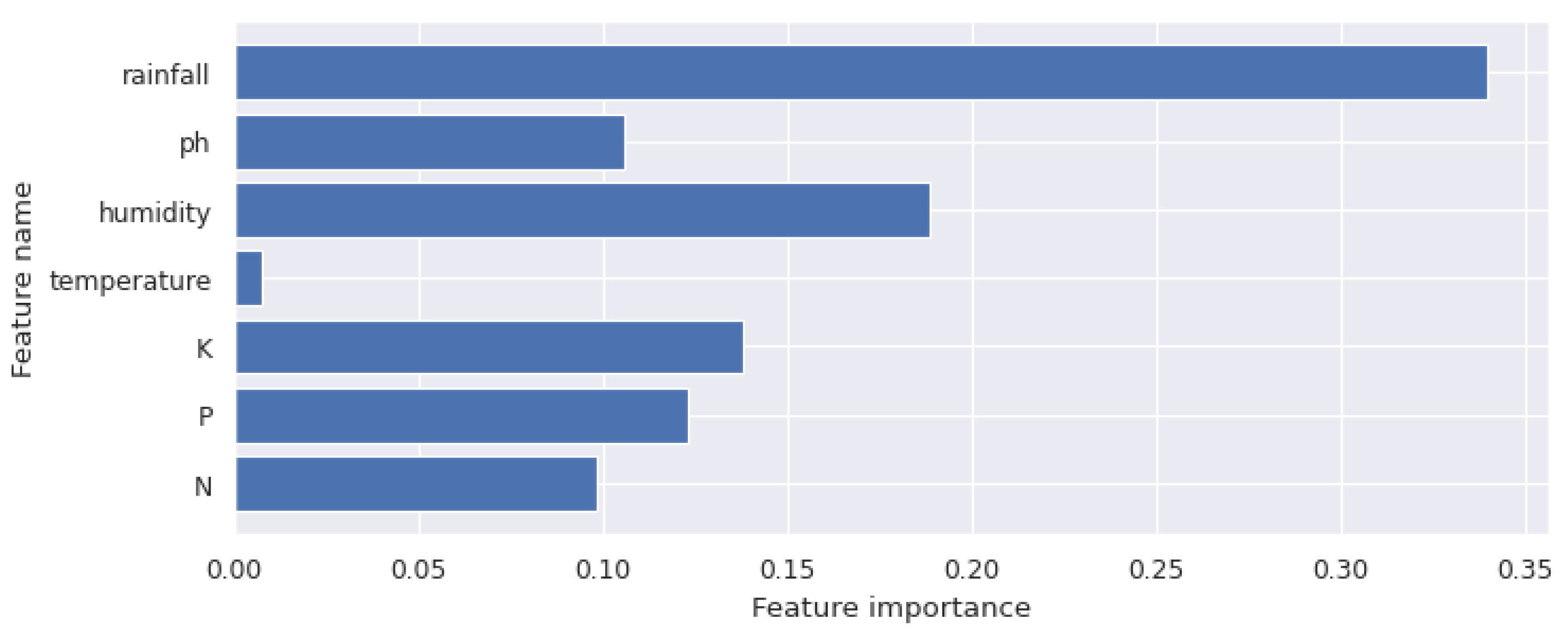
To check the balance of the dataset in the train test process of classification, 2-fold cross-validation and 10-fold cross-validation were performed. Furthermore, feature importance was computed for every feature using Algorithm 1. Figure 9 shows the feature importance [51] for the features used in this study.

Algorithm 1 Feature Importance (FI) computation

Input: Trained model (F), feature matrix ($\alpha$), target class ($\beta$), error measure ($L(\beta ,F(\alpha \left)\right)$) Output: Set of feature importance ($\xi \left(FI\right)$) 1: procedureGenerate—$\xi \left(FI\right)$ 2:     Estimate initial error, $er{r}_o$ = $L(\beta ,F(\alpha \left)\right)$ 3:     for each feature $j\in$ M do 4:         Generate feature matrix ${\alpha }_p$; ∀ j ∈ $\alpha$. 5:         Estimate error, $er{r}_e$ = $L({\beta }^{\Theta },F\left({\alpha }_p\right))$ 6:         Compute $F{I}_j=\frac{er{r}_e}{er{r}_o}$ 7:     end for 8:     Sort $F{I}_j$ and keep in the set $\xi \left(FI\right)$ 9: end procedure

3. Results

This part of the study summarizes the crop identification tests conducted using all of the machine learning algorithms outlined in the previous section. To guarantee that the machine learning algorithm’s parameters were allocated randomly at the beginning of the trial, the tests were performed 10 times. Throughout all of the studies, consistent findings have been shown.

From

Table 1. Accuracy table of all the algorithms for each crop type using 2-fold cross-validation.

Crop Type	k-NN (%)	SVM (%)	DT (%)	RF (%)	GB (%)
Rice	82.85	84.64	94.64	93.78	95.08
Maize	89.89	96.98	97.84	96.50	99.78
Chickpea	98.67	99.76	99.10	96.55	98.75
Kidneybeans	99.79	99.81	99.92	95.57	99.85
Pigeonpeas	85.45	98.54	95.54	94.88	98.94
Mothbeans	84.26	87.34	89.50	90.10	91.77
Mungbean	89.89	89.31	95.47	93.78	99.08
Blackgram	95.66	98.88	96.84	96.50	97.78
Lentil	96.89	99.42	99.10	99.55	94.75
Pomegranate	93.56	99.81	99.92	97.57	96.85
Banana	89.89	91.54	99.54	99.88	99.94
Mango	96.89	99.34	91.50	99.10	99.77
Grapes	97.29	99.31	89.47	95.78	96.08
Watermelon	89.69	99.88	99.84	99.50	99.78
Muskmelon	98.87	99.42	99.10	99.55	99.75
Apple	97.75	99.81	99.92	99.57	99.85
Orange	96.92	99.54	99.54	99.88	99.94
Papaya	98.34	99.34	99.50	99.10	99.77
Coconut	96.36	99.31	99.47	99.78	99.08
Cotton	99.16	99.88	99.84	99.50	99.78
Jute	91.67	96.42	99.10	97.55	94.75
Coffee	95.79	99.81	95.92	99.57	96.85

and

Table 2. Accuracy table of all the algorithms for each crop type using 10-fold cross-validation.

Crop Type	k-NN (%)	SVM (%)	DT (%)	RF (%)	GB (%)
Rice	94.81	95.27	91.19	90.81	99.08
Maize	99.74	97.79	98.41	97.68	99.78
Chickpea	98.87	99.76	99.24	97.81	98.75
Kidneybeans	99.79	99.81	99.92	98.15	99.85
Pigeonpeas	97.35	98.54	98.23	97.41	98.94
Mothbeans	91.78	92.45	91.20	91.12	99.77
Mungbean	99.81	99.31	91.36	93.16	99.08
Blackgram	97.66	98.88	98.46	96.50	99.78
Lentil	99.81	99.42	99.14	99.55	99.75
Pomegranate	98.56	99.81	99.92	97.57	99.85
Banana	99.89	99.54	99.54	99.88	99.94
Mango	99.89	99.34	91.50	99.10	99.77
Grapes	98.29	99.31	96.22	95.78	99.08
Watermelon	99.69	99.88	99.84	99.50	99.78
Muskmelon	99.87	99.42	99.10	99.55	99.75
Apple	99.75	99.81	99.92	99.57	99.85
Orange	99.92	99.54	99.54	99.88	99.94
Papaya	99.34	99.34	99.50	99.10	99.77
Coconut	99.36	99.31	99.47	99.78	99.08
Cotton	99.16	99.88	99.84	99.50	99.78
Jute	95.32	97.31	99.10	97.55	98.21
Coffee	99.79	99.81	95.92	99.57	99.21

, it is visible that the Gradient-boosted trees approach outperforms all the other methods in most of the cases; the accuracy score increases with the number of folds along with the F1-score.

Table 3. Evaluation criterion table for 2-fold cross-validation.

Model	Avg. Precision (%)	Avg. Recall (%)	Avg. Accuracy (%)	F1-Score (%)
k-NN	94.45	93.01	93.88	93.72
SVM	93.57	97.71	96.55	95.69
DT	97.14	96.62	97.30	97.08
RF	97.81	97.11	97.35	97.46
GB	98.78	99.62	98.13	99.20

and

Table 4. Evaluation criterion table for 10-fold cross-validation.

Model	Avg. Precision (%)	Avg. Recall (%)	Avg. Accuracy (%)	F1-Score (%)
k-NN	97.05	98.12	97.12	97.75
SVM	93.71	98.57	98.71	96.11
DT	97.28	97.22	98.77	97.24
RF	98.33	98.35	98.80	98.34
GB	99.12	98.62	99.11	98.87

show the algorithms’ performance using the already discussed evacuation criterion.

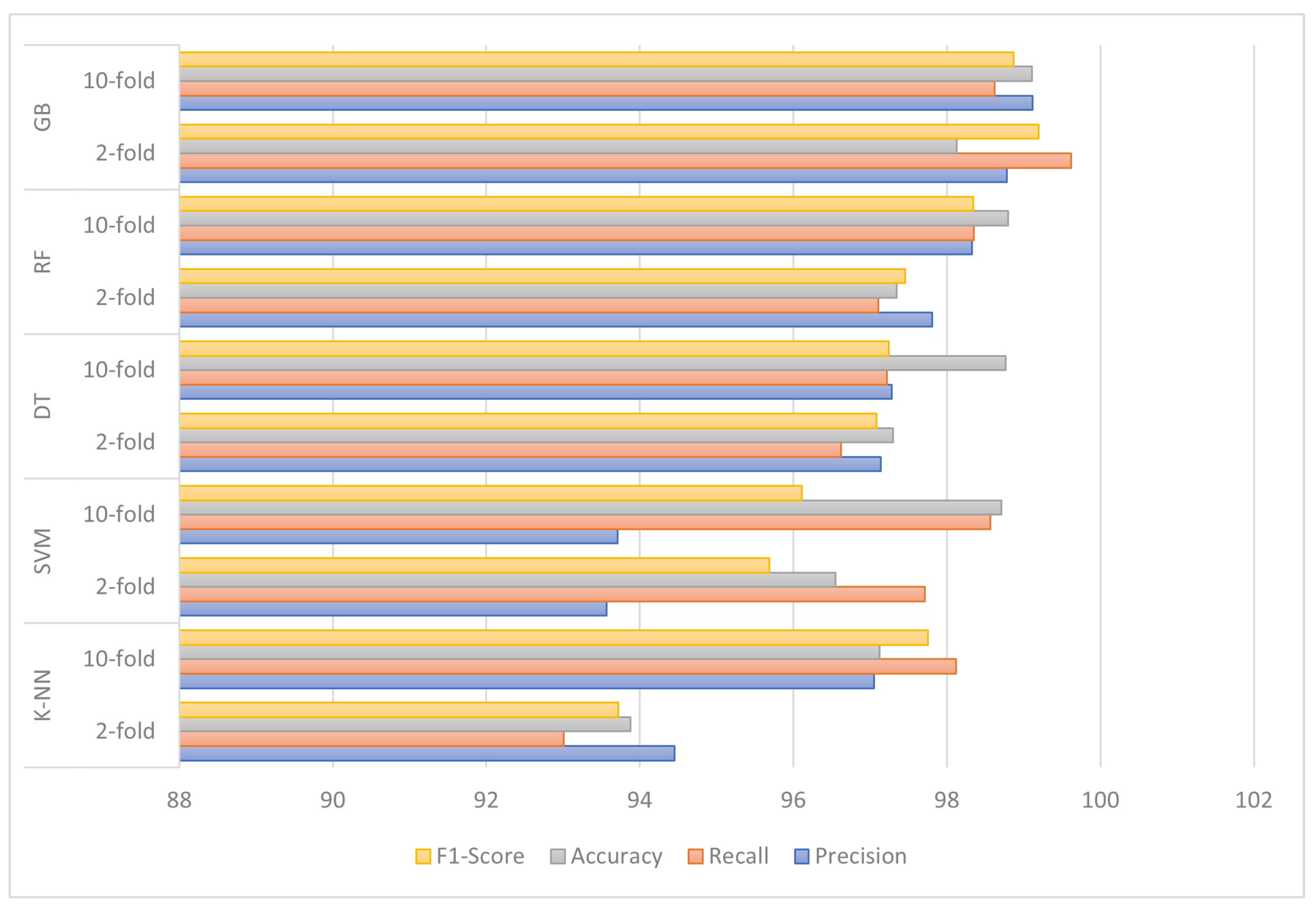
The comparative analysis of the study is shown in Figure 10.

The implementation of k-NN was executed with the value of k = 4, as shown in Figure 8. As various kernels are available for SVM, the experiment was performed for all the kernels along with parameter tuning. The parameter ’C’ was tuned for the values [0.001, 0.01, 0.1, 1.0, 10.0, 100.0], and ’gamma’ for the values [0.001, 0.01, 0.1, 1.0, 10.0, 100.0]. The performance evaluation for different kernels is shown in

Table 5. Overall Performance Assessment for SVM using different kernels.

Kernel	Avg. Precision (%)	Avg. Recall (%)	Avg. Accuracy (%)	F1-Score (%)	Parameter ‘C’	Parameter ‘Gamma’
Linear	97.45	98.01	97.44	97.75	-	-
Polynomial	83.57	81.71	77.44	82.63	-	-
Sigmoid	16.14	14.62	15.27	15.38	-	-
RBF	71.81	69.11	65.45	70.44	-	-
Linear(tuned)	98.31	98.21	97.67	98.28	01.0	0.001
Polynomial (tuned)	98.54	98.33	98.60	98.52	01.0	0.010
Sigmoid(tuned)	96.11	97.38	98.72	96.75	10.0	0.010
RBF(tuned)	98.44	98.98	98.91	98.71	01.0	0.010

. It is clear that GB trees outperform all the algorithms with an accuracy of 99.11% and an F1-score of 99.20%.

4. Discussion

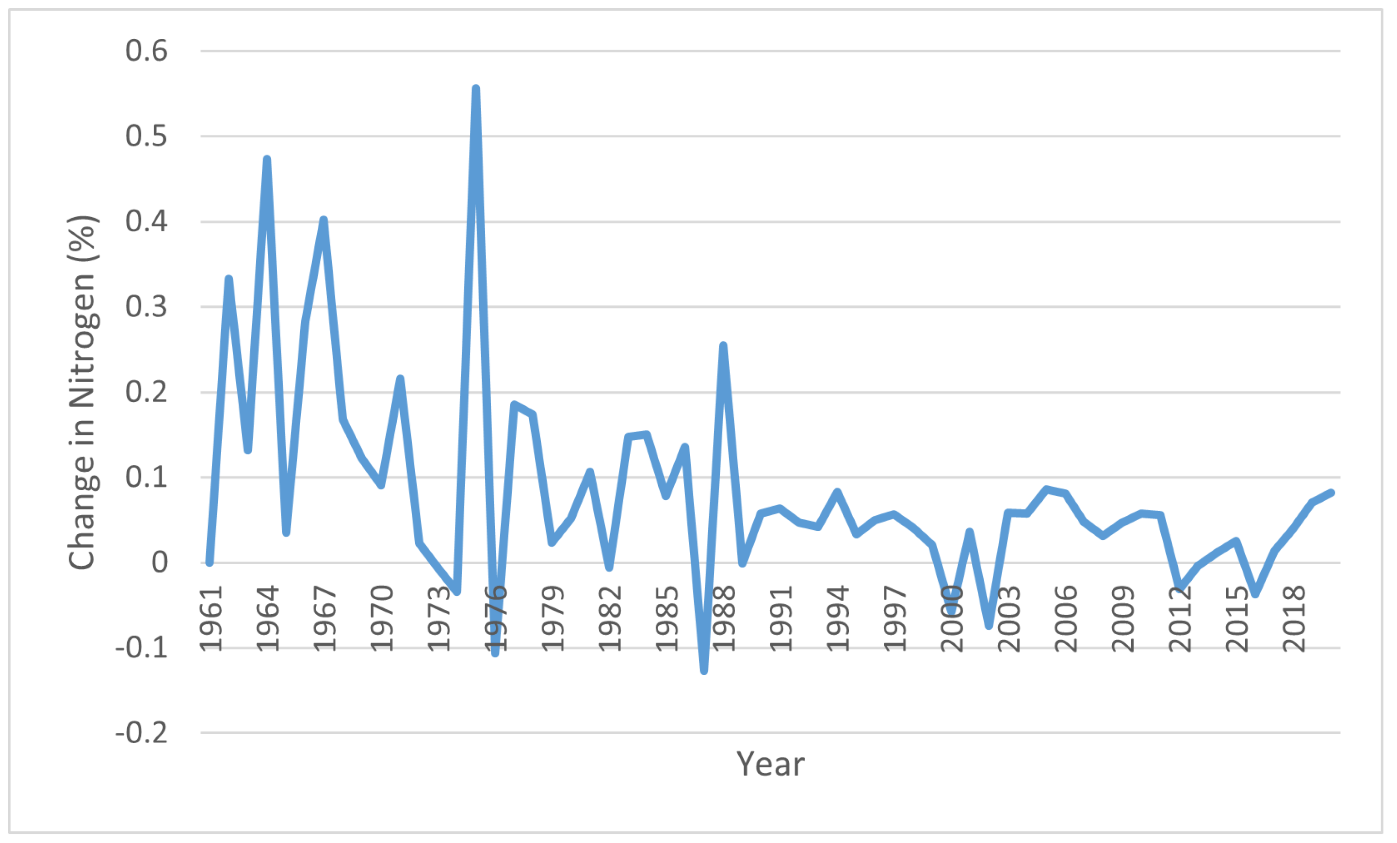
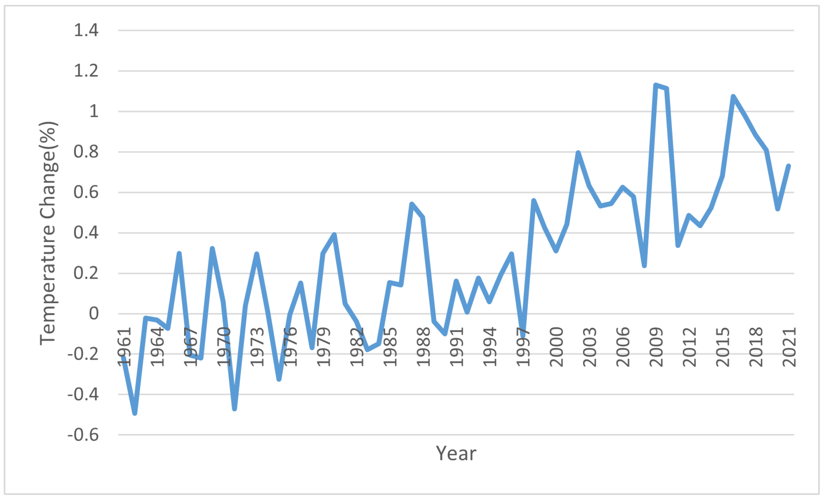
Taking India as the geographical location of our study, we collected crop data bearing soil and climate attributes since 1962. It is seen in the literature that the machine learning techniques on geospatial data were focused on other countries except for India. Moreover, researchers were concentrating more on crop yield rather than crop selection. In our study, we take the help of an Indian crop dataset integrated with other soil-based and weather-based attributes to classify the crop type. India is an agricultural economy-based country, and not a high variation in temperature and soil quality is observed. However, this is a major concern in the upcoming years. Figure 11 depicts the change in nitrogen nutrients and Figure 12 depicts the temperature change in percentage throughout the last 60 years. It is worth mentioning that the authors have not taken the variable of artificial fertilizers to be added to the soil, as it is not a part of the study.

It is seen that the ‘temperature’ and ‘pH’ show a normal distribution. In contrast, the ‘ratio of nitrogen contents’, ‘ratio of phosphorous contents’, ‘ratio of potassium contents’, and ‘rainfall in mm’ do not follow a normal distribution. Joint plots show how the attributes impact crop cultivation. For example, rice is seen to be cultivated with a relative humidity of 80%, and rainfall ranges from 150 mm to 300 mm. This is a geographical reason why rice is grown on the eastern coast of India. Similarly, kidney beans’ relative humidity and rainfall requirements are low compared to rice. The coastal regions of India export coconuts as a significant source because the humidity is very high. The impact of the potassium ‘K’ ratio and nitrogen ‘N’ contents in soil for specific crops are also seen. The effect of the pH value of the soil is analyzed. For good cultivation, a value between 6 and 7 is recommended. Due to the presence of both standard normal and other distribution of attributes in our data, we used Pearson’s correlation coefficient for normally distributed attributes and Spearman’s correlation coefficient for the attributes which are not normal. The potassium and phosphorous ratios are highly correlated, which indicates essential characteristics of the Indian soil.

Distance algorithms such as KNN, K-means, and SVM are affected by a large number of different parameters because comparisons of data points are made based on how closely they are situated to one another. Hence, we use the min-max feature scaling. Now, we can reduce the impact of outlier data for distributions that are not normal on our model by using the normalization technique. We computed the importance of each attribute using the feature importance algorithm and observed that ‘rainfall’ is the most crucial attribute in our dataset. Finally, we implement the machine learning algorithms in our dataset to create a classification model of the crop type based on the characteristics. We observed in the previous section that the GB tree was performing best as it scored the highest in the evaluation criterion.

The findings will aid farmers in selecting the best crop for their region’s soil and climate. As India is an agricultural country, we trained our artificial intelligence models based on the features and data of the country. Keeping sustainable farming in focus, the farmers of land could measure the soil characteristics and give them as input to our system. The system will guide the farmers in selecting the most suitable crop based on the land characteristics and the climate.

Based on this study, more work has to be done to account for other factors that affect crop variety and yield. In the future, we will include the crop yield and the type prediction with the probability of disease in the crop. Deep learning methods will be deployed to improve crop selection accuracy by factoring in yield and fertilizer consumption.

5. Conclusions

This research aims to predict the type of crop in the Indian context for cultivation given the rainfall and humidity of weather conditions along with the ratio of nitrogen, phosphorous, potassium, and pH value of soil. In the proposed study, various conventional machine learning algorithms were used to recognize the type of crop required for plantation, given the conditions.

The proposed work aims to statistically study the attributes’ role and impact on crops’ growth. We found very interesting observations like how humidity and rainfall in various geographical locations in India lead to the cultivation of some specific crops, as well as how potassium and nitrogen content ratio in the soil help in crop selection. The most important attribute was ‘rainfall’, which was found using a feature selection algorithm. Various machine learning algorithms like k-NN, SVM, RF, and GB trees were compared to predict the crop type. The GB tree method gave the best accuracy of 99.11% which is significant for building an accurate crop prediction system. However, there is still a need for improvement with other attributes contributing to the crop type with different yields. In the future, we aim to incorporate the yield and use of fertilizers in the crop selection methodology and try to increase the accuracy by using deep learning techniques.

References

- Kc, S.; Wurzer, M.; Speringer, M.; Lutz, W. Future population and human capital in heterogeneous India. Proc. Natl. Acad. Sci. USA 2018, 115, 8328–8333. [Google Scholar] [CrossRef] [PubMed] [Green Version]
- Samaddar, A.; Cuevas, R.P.; Custodio, M.C.; Ynion, J.; Ray, A.; Mohanty, S.K.; Demont, M. Capturing diversity and cultural drivers of food choice in eastern India. Int. J. Gastron. Food Sci. 2020, 22, 100249. [Google Scholar] [CrossRef] [PubMed]
- Sharma, B.R.; Gulati, A.; Mohan, G.; Manchanda, S.; Ray, I.; Amarasinghe, U. Water Productivity Mapping of Major Indian Crops. 2018. Available online: http://hdl.handle.net/11540/8480 (accessed on 17 October 2022).
- Malik, A.; Dwivedi, N. An analytic study of Indian agriculture Crop with reference to wheat. Int. J. Mod. Agric. 2021, 10, 2164–2172. [Google Scholar]
- Chatterjee, S.; Chaudhuri, R.; Vrontis, D. Managing knowledge in Indian Organizations: An empirical investigation to examine the moderating role of jugaad. J. Bus. Res. 2022, 141, 26–39. [Google Scholar] [CrossRef]
- Chattopadhyay, A.; Khan, J.; Bloom, D.E.; Sinha, D.; Nayak, I.; Gupta, S.; Lee, J.; Perianayagam, A. Insights into Labor Force Participation among Older Adults: Evidence from the Longitudinal Ageing Study in India. J. Popul. Ageing 2022, 15, 39–59. [Google Scholar] [CrossRef]
- Panigrahi, R. Trends in Agricultural Production and Productivity Growth in India: Challenges to Sustainability. In Business Governance and Society; Palgrave Macmillan: Cham, Switzerland, 2019; pp. 17–28. [Google Scholar]
- Subudhi, H.N.; Prasad, K.V.S.V.; Ramakrishna, C.; Rameswar, P.S.; Pathak, H.; Ravi, D.; Khan, A.A.; Padmakumar, V.; Blümmel, M. Genetic variation for grain yield, straw yield and straw quality traits in 132 diverse rice varieties released for different ecologies such as upland, lowland, irrigated and salinity prone areas in India. Field Crops Res. 2020, 245, 107626. [Google Scholar] [CrossRef]
- Mc Carthy, U.; Uysal, I.; Badia-Melis, R.; Mercier, S.; O’Donnell, C.; Ktenioudaki, A. Global food security–Issues, challenges and technological solutions. Trends Food Sci. Technol. 2018, 77, 11–20. [Google Scholar] [CrossRef]
- Bach, H.; Wolfram, M. Sustainable agriculture and smart farming. In Earth Observation Open Science and Innovation; Springer: Cham, Switzerland, 2018; pp. 261–269. [Google Scholar]
- Heitlinger, S.; Bryan-Kinns, N.; Comber, R. The right to the sustainable smart city. In Proceedings of the 2019 CHI Conference on Human Factors in Computing Systems, Glasgow, UK, 4–9 May 2019. [Google Scholar]
- Ahad, M.A.; Paiva, S.; Tripathi, G.; Feroz, N. Enabling technologies and sustainable smart cities. Sustain. Cities Soc. 2020, 61, 102301. [Google Scholar] [CrossRef]
- Ali, M.; Mubeen, M.; Hussain, N.; Wajid, A.; Farid, H.U.; Awais, M.; Hussain, S.; Akram, W.; Amin, A.; Akram, R.; et al. Role of ICT in crop management. In Agronomic Crops; Springer: Singapore, 2019; pp. 637–652. [Google Scholar]
- Smith, M.J. Getting value from artificial intelligence in agriculture. Anim. Prod. Sci. 2018, 60, 46–54. [Google Scholar] [CrossRef]
- Dahikar, S.S.; Rode, S.V. Agricultural crop yield prediction using artificial neural network approach. Int. J. Innov. Res. Electr. Electron. Instrum. Control. Eng. 2014, 2, 683–686. [Google Scholar]
- Khaki, S.; Wang, L. Crop yield prediction using deep neural networks. Front. Plant Sci. 2019, 10, 621. [Google Scholar] [CrossRef] [PubMed] [Green Version]
- Winston, P.H. Artificial Intelligence; Addison-Wesley Longman Publishing Co., Inc.: Boston, MA, USA, 1992. [Google Scholar]
- Jordan, M.I.; Mitchell, T.M. Machine learning: Trends, perspectives, and prospects. Science 2015, 349, 255–260. [Google Scholar] [CrossRef] [PubMed]
- Liakos, K.G.; Busato, P.; Moshou, D.; Pearson, S.; Bochtis, D. Machine learning in agriculture: A review. Sensors 2018, 18, 2674. [Google Scholar] [CrossRef] [PubMed] [Green Version]
- Jha, K.; Doshi, A.; Patel, P.; Shah, M. A comprehensive review on automation in agriculture using artificial intelligence. Artif. Intell. Agric. 2019, 2, 1–12. [Google Scholar] [CrossRef]
- Bannerjee, G.; Sarkar, U.; Das, S.; Ghosh, I. Artificial intelligence in agriculture: A literature survey. Int. J. Sci. Res. Comput. Sci. Appl. Manag. Stud. 2018, 7, 1–6. [Google Scholar]
- Dharmaraj, V.; Vijayanand, C. Artificial intelligence (AI) in agriculture. Int. J. Curr. Microbiol. Appl. Sci. 2018, 7, 2122–2128. [Google Scholar] [CrossRef]
- Patrício, D.I.; Rieder, R. Computer vision and artificial intelligence in precision agriculture for grain crops: A systematic review. Comput. Electron. Agric. 2018, 153, 69–81. [Google Scholar] [CrossRef] [Green Version]
- Bhuyan, B.P.; Tomar, R.; Gupta, M.; Ramdane-Cherif, A. An Ontological Knowledge Representation for Smart Agriculture. In Proceedings of the 2021 IEEE International Conference on Big Data (Big Data), Orlando, FL, USA, 15–18 December 2021. [Google Scholar] [CrossRef] [Green Version]
- Bhuyan, B.P.; Tomar, R.; Cherif, A.R. A Systematic Review of Knowledge Representation Techniques in Smart Agriculture (Urban). Sustainability 2022, 14, 15249. [Google Scholar] [CrossRef]
- Kim, N.; Ha, K.J.; Park, N.W.; Cho, J.; Hong, S.; Lee, Y.W. A comparison between major artificial intelligence models for crop yield prediction: Case study of the midwestern United States, 2006–2015. ISPRS Int. J. Geo-Inf. 2019, 8, 240. [Google Scholar] [CrossRef] [Green Version]
- Khairunniza-Bejo, S.; Mustaffha, S.; Ismail WI, W. Application of artificial neural network in predicting crop yield: A review. J. Food Sci. Eng. 2014, 4, 1. [Google Scholar]
- Babaee, M.; Maroufpoor, S.; Jalali, M.; Zarei, M.; Elbeltagi, A. Artificial intelligence approach to estimating rice yield. Irrig. Drain. 2021, 70, 732–742. [Google Scholar] [CrossRef]
- Yaramasu, R.; Bandaru, V.; Pnvr, K. Pre-season crop type mapping using deep neural networks. Comput. Electron. Agric. 2020, 176, 105664. [Google Scholar] [CrossRef]
- Pott, L.P.; Amado TJ, C.; Schwalbert, R.A.; Corassa, G.M.; Ciampitti, I.A. Satellite-based data fusion crop type classification and mapping in Rio Grande do Sul, Brazil. ISPRS J. Photogramm. Remote. Sens. 2021, 176, 196–210. [Google Scholar] [CrossRef]
- Zhang, C.; Di, L.; Lin, L.; Guo, L. Machine-learned prediction of annual crop planting in the US Corn Belt based on historical crop planting maps. Comput. Electron. Agric. 2019, 166, 104989. [Google Scholar] [CrossRef]
- Potgieter, A.B.; Zhao, Y.; Zarco-Tejada, P.J.; Chenu, K.; Zhang, Y.; Porker, K.; Biddulph, B.; Dang, Y.P.; Neale, T.; Roosta, F.; et al. Evolution and application of digital technologies to predict crop type and crop phenology in agriculture. In Silico Plants 2021, 3, Diab017. [Google Scholar] [CrossRef]
- de Jong, S. Crop Type Prediction Based on Farmers Declarations. Master’s Thesis, Utrecht University, Utrecht, The Netherlands, 2018. [Google Scholar]
- Mohan, P.; Patil, K.K. Deep learning based weighted SOM to forecast weather and crop prediction for agriculture application. Int. J. Intell. Eng. Syst. 2018, 11, 167–176. [Google Scholar] [CrossRef]
- Dimov, D. Classification of remote sensing time series and similarity metrics for crop type verification. J. Appl. Remote. Sens. 2022, 16, 024519. [Google Scholar] [CrossRef]
- Orynbaikyzy, A.; Gessner, U.; Conrad, C. Spatial Transferability of Random Forest Models for Crop Type Classification Using Sentinel-1 and Sentinel-2. Remote Sens. 2022, 14, 1493. [Google Scholar] [CrossRef]
- Han, X.; Wei, Z.; Zhang, B.; Li, Y.; Du, T.; Chen, H. Crop evapotranspiration prediction by considering dynamic change of crop coefficient and the precipitation effect in back-propagation neural network model. J. Hydrol. 2021, 596, 126104. [Google Scholar] [CrossRef]
- Ringen, J. FAO, the United Nations Food and Agricultural Organisation. Tidsskr. Nor. Landbr. 1946, 53, 287–304. [Google Scholar]
- Kar, G.; Sahoo, N.; Kumar, A. Deep-water rice production as influenced by time and depth of flooding on the east coast of India. Arch. Agron. Soil Sci. 2012, 58, 573–592. [Google Scholar] [CrossRef]
- Kumar, S.N.; Aggarwal, P.K. Aggarwal. Climate change and coconut plantations in India: Impacts and potential adaptation gains. Agric. Syst. 2013, 117, 45–54. [Google Scholar] [CrossRef]
- Hauke, J.; Kossowski, T. Comparison of values of Pearson’s and Spearman’s correlation coefficient on the same sets of data. Quaest. Geogr. 2011, 30, 87. [Google Scholar] [CrossRef] [Green Version]
- Patro, S.; Sahu, K.K. Normalization: A preprocessing stage. arXiv 2015, arXiv:1503.06462. [Google Scholar] [CrossRef]
- Ali, M.; Jung, L.T.; Abdel-Aty, A.H.; Abubakar, M.Y.; Elhoseny, M.; Ali, I. Semantic-k-NN algorithm: An enhanced version of traditional k-NN algorithm. Expert Syst. Appl. 2020, 151, 113374. [Google Scholar] [CrossRef]
- Noble, W.S. What is a support vector machine? Nat. Biotechnol. 2006, 24, 1565–1567. [Google Scholar] [CrossRef]
- Quinlan, J.R. Learning decision tree classifiers. ACM Comput. Surv. (CSUR) 1996, 28, 71–72. [Google Scholar] [CrossRef]
- Belgiu, M.; Drăguţ. Random forest in remote sensing: A review of applications and future directions. ISPRS J. Photogramm. Remote. Sens. 2016, 114, 24–31. [Google Scholar] [CrossRef]
- Ye, J.; Chow, J.H.; Chen, J.; Zheng, Z. Stochastic gradient boosted distributed decision trees. In Proceedings of the 18th ACM Conference on Information and Knowledge Management, Hong Kong, China, 2–6 November 2009. [Google Scholar]
- Charoen-Ung, P.; Mittrapiyanuruk, P. Sugarcane yield grade prediction using random forest and gradient boosting tree techniques. In Proceedings of the 2018 15th International Joint Conference on Computer Science and Software Engineering (JCSSE), Nakhonpathom, Thailand, 11–13 July 2018. [Google Scholar]
- Betke, M.; Wu, Z. Evaluation criteria. In Data Association for Multi-Object Visual Tracking; Springer: Cham, Switzerland, 2017; pp. 29–35. [Google Scholar]
- Dziak, J.J.; Coffman, D.L.; Lanza, S.T.; Li, R.; Jermiin, L.S. Sensitivity and specificity of information criteria. Briefings Bioinform. 2020, 21, 553–565. [Google Scholar] [CrossRef]
- Wojtas, M.; Chen, K. Feature importance ranking for deep learning. Adv. Neural Inf. Process. Syst. 2020, 33, 5105–5114. [Google Scholar]
Figure 1.
Probability distribution curves of the attributes where the y-axis denotes the probability and the x-axis presents the corresponding attribute. Here, the attributes are: N—the ratio of Nitrogen content in soil; P—the ratio of Phosphorous content in soil; K—the ratio of Potassium content in soil; temperature—the temperature in degrees Celsius; humidity—relative humidity in %; pH—pH value of the soil; rainfall—rainfall in mm.
Figure 2.
Diagonal distribution of the attributes.
Figure 3.
Impact of Humidity and Rainfall in certain crops.
Figure 4.
Impact of the ratio of potassium ‘K’ and nitrogen ‘N’ contents in soil for certain crops.
Figure 5.
Impact of pH level.
Figure 6.
Pearson’s correlation coefficient heat map between the attributes.
Figure 7.
Spearman’s correlation coefficient heat map between the attributes.
Figure 8.
Accuracy of prediction vs value of ‘k’.
Figure 9.
Feature importance.
Figure 10.
Comparative analysis between the classification algorithms after 2-fold and 10-fold validation concerning the evaluation criterion.
Figure 11.
Nitrogen nutrient change in soil (percentage) throughout the last 60 years.
Figure 12.
Temperature change in India (percentage) throughout the last 60 years.