A Quantitative Study on Driving Behavior Economy Based on Big Data from the Pure Electric Bus

Abstract

In order to help improve the economy, energy savings and emission reductions of pure electric buses, based on the driving data, a new driving cycle construction method is proposed. Through the dividing of short trips and the calculation of characteristic parameter values, two typical driving conditions (weekday driving condition and weekend driving condition) are constructed via principal components analysis and the k-means clustering method, and both have a high degree of compatibility with the actual conditions. Based on the two typical driving conditions, the CRITIC (Criteria Importance Through Intercriteria Correlation) method and the quantitative analysis are used to establish a quantitative evaluation model to score the economy of the driver’s driving behavior. The result shows that the weekend working condition with the better traffic environment promotes the generation of aggressive driving behavior and increases the random fluctuation seen in the driver’s driving process: for the weekend driving condition, the proportion of low economic efficiency is about 4.5 times bigger than the proportion on weekdays, and the former’s fluctuation range for the driving behavior score is 37% higher than that of the latter, meaning that the overall economy of the pure electric bus is much worse on weekends.

1. Introduction

The typical driving condition and driving behavior characteristic are two important factors that affect the economy of the pure electric bus. The former affects the selection of vehicle parameters during the vehicle design stage, where the economic performance of the vehicle is determined directly by whether or not the powertrain parameters are suitable for the typical working conditions of the target market; the latter affects the vehicle energy consumption during the vehicle operation stage, reflecting the impact of driving behavior on the bus economy. Based on the two aspects [1,2], the quantitative performance of the driver’s driving behavior under different working conditions has been analyzed to help improve the economy of the pure electric bus in the future.

For driving conditions, the standard driving cycles (such as NEDC, CHTC-B, WLTC and EPA, etc.) published at home and abroad are significantly different from the local line conditions, thus the actual driving process of local vehicles cannot be reflected accurately. Due to the existence of regional variability, the typical driving conditions established for specific lines have higher accuracy and applicability than the standard ones [3,4,5,6]. Furthermore, the typical driving conditions obtained by different construction methods have different driving characteristics, which makes a large deviation in the final economic evaluation [7]. Therefore, increasing the consistency between typical working conditions and actual line conditions as much as possible is an urgent problem.

However, current studies may be further improved cause they can be divided into two types: general type and detail type. The general type [1,3,5,6,7,8] treats all the collected data as the same type and tries to construct one working condition to adapt to every driving environment. It shows small errors on large amounts of data but may generate large errors in actual daily operations. The detail type [4,9,10] tries to divide the driving data into several types, such as peak and off-peak data. This method is easy to operate and has the advantage of a high differentiation of driving conditions, but the criteria of dividing peak data and off-peak data is vague, and the integrity of the bus driving conditions has consequently been destroyed. Therefore, this study proposes a new method of constructing driving conditions within specific time dimensions to avoid such problems and to improve the consistency between typical working conditions and actual line conditions. The method treats driving data from Monday to Friday as the same type and those from Saturday to Sunday as another; thus, two working conditions are basically enabled to describe the driving environment of buses on any given day and to solve the problem of general-type studies to a large extent. Additionally, by applying this method the data integrality of each day is reserved instead of splitting all the collected data into pieces, such as into peak and off-peak data. Although during a week there would be some holidays or special events that may change the driving environment, these two working conditions are effective enough for bus companies to launch vehicle tests.

Additionally, road conditions tend to produce certain hints and inducements to the driver’s psychology, resulting in positive or negative emotions and a tendency to adopt more aggressive driving behaviors [11,12]. Under the influence of related emotions, the more aggressive the driver’s driving behavior, the less attention the driver pays to the surroundings, and the higher the frequency of rapid acceleration and deceleration [13]. This increase in the frequency means more energy consumption and a low vehicle economy as well as damage to the battery remain life, which is not acceptable for bus companies. Therefore, in order to regulate the driver’s driving behavior and provide reference for subsequent personnel management, the aggressiveness of drivers’ driving styles should be evaluated by selecting certain indicators [14]. With reference to the eco-driving concept [15,16], in ref. [17] seven indicators were selected and processed with a prediction model explainer to allocate eco-drive scores, resulting in an average vehicle economy improvement of 12.1%; Andrieu et al. [18] constructed an aggregated indicator using the probability of being an eco-driver to obtain an eco-index and can be useful for driver monitoring; furthermore, an Elman neural network was applied to establish a driving behavior economy evaluation model based on four economy indicators in [19]; in ref. [20], eight indicators associated with the vehicle’s speed, acceleration, driving time and so on were chosen to objectively assess the driver’s driving style and could improve the driver’s behavior behind the wheel. These evaluation methods and models have achieved relatively good results [21] and reflected the actual driving situation of drivers to a certain extent, but they put too much emphasis on the driver themselves and focus on reviewing the driver’s performance without referring to a reasonable working condition in which the driver is involved. To complement this, this study tries to analyze how these two different working conditions affect driver’s driving behaviors and explain why the driver takes particular actions. The contributions made by this paper are as follows:

(1)

A new effective driving cycle construction method is proposed to obtain the weekday working condition and the weekend working condition via PCA and k-means clustering. It reserves the data integrality of each day, reflects the changing cycle of bus working condition and achieves a clearer and simpler criterion for data dividing during the construction of working conditions.

(2)

A quantitative evaluation model is established to score the economy of the driver’s driving behavior with the CRITIC method. Five new indicators are chosen to evaluate the driving performance of the driver. The result is consistent with the constructed working conditions.

(3)

The two working conditions have different effects on the driver’s psychology, resulting in different driving behaviors, of which the reasons for have been pointed out. They provide new viewpoints to analyze and strengthen the connection between working conditions and driver’s driving behavior, which would be good references for economy improving.

In summary, with the measured bus operating data, this study first proposes a new way to construct working conditions for the pure electric bus by using weekday driving data as the basis for constructing weekday working conditions and the weekend driving data for weekend working conditions; then the quantitative performance of the driver’s driving behavior economy is analyzed based on the two working conditions to investigate the specific link between road conditions and driving behavior economy.

2. Data Acquisition and Processing

2.1. Data Acquisition

The driving data are collected from an electric bus operating in Guangzhou (China) and the collection time is from 7:00 a.m. to 20:00 p.m. on weekdays and 7:00 a.m. to 24:00 p.m. on weekends. Sampling every 0.2 s, the initial data are 160,892 (weekday) and 233,217 (weekend), covering 197 dimensions (such as date, longitude and latitude, vehicle speed, mileage, energy consumption, pedal information, motor information, battery temperature, etc.) The bus operation route is shown in Figure 1, which connects the Tianhe terminal and Nanhu terminal and passes through some complex traffic sections such as urban areas, suburban areas, universities, subway stations and 5 A scenic spots. With moderate length and a reasonable number of stations, it has strong representativeness among many other lines and is chosen as the object of this study.

The bus is GAC BYD K8 (GZ6100LGEV5), and its technical information is shown in

Table 1. The bus information.

Parameter	Value
Length	10,490 mm
Height	3250 mm
Width	2550 mm
Wheelbase	5000 mm
Curb weight	12,200 kg
Gross weight	18,000 kg
Tyre	275/70R22.5
Frontal area	6.79 m2
Seat	74/16–37
Max speed	69 km/h

, with the wheel-side permanent magnet synchronous motor and lithium-ion ferrous phosphate battery.

2.2. Data Pre-Processing

The initial data amounts are 160,892 (weekday) and 233,217 (weekend). First, unneeded data dimensions are deleted, such as the longitude and latitude, battery temperature and so on. A total of 193 dimensions have been removed and 4 key dimensions are reserved: time, vehicle speed, accelerator pedal opening and brake pedal opening. Meanwhile, there are some abnormal data generated during the acquisition process by the influence of road factors and the deficiencies in acquisition devices. These are mainly reflected in the empty speed values, non-zero idle speed and unreasonable bus speed.

However, due to the high sampling frequency, the empty value amount in the data used is zero and the largest value is still within reasonable limits, so there is no abnormal bus speed in the dataset. The non-zero idle speed mainly influences the short trips division and appears once or twice among many zero-seconds readings, so they are identified and ignored as zero in the python program. Then, the data granularity is adjusted to 1 Hz by calculating the mean values (4–5 data in one second are calculated as one mean value data figure). During this process 125,746 data (weekday) and 182,026 data (weekend) are merged into the mean data.

After the data pre-processing, the data dimensions are changed from 197 to 4, and a total of 35,146 weekday mean values data and 51,011 weekend mean values data are retained in the end.

3. Working Conditions Construction

3.1. Short Trips and Feature Variables

3.1.1. Short Trips Division

A short trip means a process of movement from the start of one idling phase to the next idling phase, as shown by Figure 2. Additionally, the whole driving process of a pure electric bus can be broken into multiple short trips, each of which consists of two parts: the idle phase and the driving phase. The driving phase can be further divided into the acceleration period, the uniform period and the deceleration period [22].

The Python program is used to detect the start and end moments of each short trip, dividing the whole driving data into desired short trip segments.

3.1.2. Feature Variables Calculation

To describe the time and velocity characteristics of each short trip, as well as the proportional relations of each component to the whole, a total of 24 feature variables are selected as shown in

Table 2. Feature variables of the short trip.

Number	Feature Variable	Symbol
1	Mileage	S/km
2	Total time	T/s
3	Acceleration time	Tup/s
4	Deceleration time	Td/s
5	Uniform time	Tu/s
6	Idle time	Ts/s
7	Maximum speed	Vmax/(km/h)
8	Average speed	Va/(km/h)
9	Average driving speed	Vwa/(km/h)
10	Standard deviation of speed	Vsd
11	Maximum acceleration	amax/(m/s2)
12	Maximum deceleration	amin/(m/s2)
13	Average acceleration of the acceleration period	aupa/(m/s2)
14	Average deceleration of the deceleration period	ada/(m/s2)
15	Standard deviation of acceleration	asd
16	Proportion of 0–10 km/h speed	P1
17	Proportion of 10–20 km/h speed	P2
18	Proportion of 20–30 km/h speed	P3
19	Proportion of 30–40 km/h speed	P4
20	Proportion of 40–50 km/h speed	P5
21	Proportion of acceleration period	Pup
22	Proportion of deceleration period	Pd
23	Proportion of uniform period	Pu
24	Proportion of idle period	Ps

.

The definitions for each driving period are given as follows [14]:

• Acceleration period: the speed is greater than 0 and the acceleration is greater than 0.12 m/s².
• Deceleration period: the speed is greater than 0 and the deceleration is less than −0.12 m/s².
• Uniform period: the vehicle speed is not 0 and the acceleration is between −0.12 m/s² and 0.12 m/s².
• Idle period: the speed is 0 and the acceleration is between −0.12 m/s² and 0.12 m/s².

3.2. Working Conditions Construction

3.2.1. Principal Component Analysis

Principal component analysis (PCA) is used to drastically reduce the dimensionality of large datasets in an interpretable way and preserve as much variability as possible [23]. So, in this part, the dimension of the feature variables is reduced to avoid the overlapping of information contained in them and at the same time reduce the repeated calculations. The specific steps are as follows:

Feature variables matrix $A_{m\times n}$:

$$A_{m\times n}=\left[\begin{array}{ccc}{a}_{11}& \dots & a_{1n}\\ ⋮& \ddots & ⋮\\ a_{m1}& \dots & a_{mn}\end{array}\right]$$

(1)

where m is the number of short trips and n is the number of feature variables. In weekday data, m is 384 and n is 24. In weekend data, the m is 563 and n is 24.

First the original feature variables need to be normalized, and the commonly used Z-score normalization method is shown as below:

$$a_{ij}^{*}=\frac{a_{ij}-{\mu }_j}{{\sigma }_j}$$

(2)

where $a_{ij}^{*}$ is the normalized parameter of $a_{ij}$, ${\mu }_j$ is the mean of this feature variable and ${\sigma }_j$ is the standard deviation of this feature variable.

Then, the normalized feature variables matrix $A_{m\times n}^{*}$ is obtained:

$$A_{m\times n}^{*}=\left[\begin{array}{ccc}{a}_{11}^{*}& \dots & a_{1n}^{*}\\ ⋮& \ddots & ⋮\\ a_{m1}^{*}& \dots & a_{mn}^{*}\end{array}\right]$$

(3)

Then, calculate the covariance matrix $C_{n\times n}$:

$$C_{n\times n}=\left[\begin{array}{ccc}{c}_{11}& \dots & c_{1n}\\ ⋮& \ddots & ⋮\\ c_{n1}& \dots & c_{nn}\end{array}\right]$$

(4)

where

$$c_{ij}=cov\left(i,j\right)=\frac{{{\displaystyle \sum }}_{k=1}^m\left(a_{ki}^{*}-{\mu }_i\right)\left(a_{kj}^{*}-{\mu }_j\right)}{m-1}$$

(5)

Then, the eigenvalues ${\lambda }_i$ (i = 1, 2, …, 24) of the matrix $C_{n\times n}$ are calculated, and the variance contribution rate $f_i$ of the i-th principal component and the cumulative contribution rate $F_i$ of the first k principal components are obtained using the following equation:

$$f_i=\frac{{\lambda }_i}{{{\displaystyle \sum }}_{i=1}^{24}{\lambda }_i}$$

(6)

$$F_i=\frac{{{\displaystyle \sum }}_{k=1}^i{\lambda }_k}{{{\displaystyle \sum }}_{i=1}^{24}{\lambda }_i}$$

(7)

The eigenvalues represent the variance of corresponding principal component, and the larger the variance value is, the more the principal component explains the original information, and the less it is correlated with the rest of the principal components.

The principal component variables with variance greater than 1 are selected as the extraction results, and five principal component variables were obtained for both weekday and weekend driving conditions. With cumulative contribution rates above 80%, these variables can be considered to have basically retained most of the information of the original feature variables. (

Table 3. Principal components and variance contribution rates (weekday).

Component	Variance	${\mathit{f}}_{\mathit{i}}$/%	${\mathit{F}}_{\mathit{i}}$/%
1	10.256	42.732	42.732
2	3.590	14.957	57.689
3	3.541	14.752	72.442
4	1.425	5.939	78.381
5	1.060	4.418	82.799
6	0.923	3.846	⋮
7	0.837	3.486	⋮
⋮	⋮	⋮	⋮
24	7.628 × 10−12	3.147 × 10−11	100

and

Table 4. Principal components and variance contribution rates (weekend).

Component	Variance	${\mathit{f}}_{\mathit{i}}$/%	${\mathit{F}}_{\mathit{i}}$/%
1	9.394	42.732	42.732
2	4.436	18.483	57.627
3	3.607	15.028	72.655
4	1.335	5.562	78.217
5	1.056	4.400	82.617
6	0.941	3.923	⋮
7	0.809	3.372	⋮
⋮	⋮	⋮	⋮
24	8.183 × 10−12	3.410 × 10−11	100

).

In Table 3, principal component 1 contains the information of 14 feature variables (Mileage, Acceleration time, Deceleration time, Uniform time, Maximum speed, Average speed, Average driving speed, Standard deviation of speed, Maximum acceleration, Proportion of 20–30 km/h speed, Proportion of 30–40 km/h speed, Proportion of acceleration, Proportion of deceleration period and Proportion of uniform period), reflecting the comprehensive characteristics of short trips.

Principal component 2 contains four feature variables (Total time, idle time, Standard deviation of acceleration and Proportion of idle period), mainly reflecting the time (especially idle time) characteristics of short trips.

Principal component 3 contains three feature variables (Maximum deceleration, Average deceleration of the deceleration period and Proportion of 0–10 km/h speed), mainly reflecting the low-speed and deceleration characteristics of short trips.

Principal component 4 contains one feature variable (Proportion of 10–20 km/h speed), mainly reflecting the middle-speed characteristic of short trips.

Principal component 5 contains two feature variables (Average acceleration of the acceleration period and Proportion of 40–50 km/h speed), mainly reflecting the high-speed and acceleration characteristics of short trips.

In Table 4, principal component 1 contains the information of 15 feature variables (Mileage, Acceleration time, Deceleration time, Uniform time, Maximum speed, Average speed, Average driving speed, Standard deviation of speed, Maximum acceleration, Proportion of 10–20 km/h speed, Proportion of 20–30 km/h speed, Proportion of 30–40 km/h speed, Proportion of acceleration period, Proportion of deceleration period and Proportion of uniform period), reflecting the comprehensive characteristics of short trips.

Principal component 2 contains two feature variables (Maximum deceleration and Average deceleration of the deceleration period), mainly reflecting the deceleration characteristic of short trips.

The principal component 3 contains six feature variables (Total time, idle time, Average acceleration of the acceleration period, Standard deviation of acceleration, Proportion of 0–10 km/h speed and Proportion of idle period), mainly reflecting the low-speed and acceleration characteristics of short trips.

Principal component 4 mainly reflects other information not relevant to the eigenvalue parameters.

Principal component 5 contains one feature variable (Proportion of 40–50 km/h speed), mainly reflecting the high-speed characteristic of short trips.

3.2.2. Cluster Analysis

Taking the principal component variables obtained above as new feature variables, the clustering of short trips can determine their categories accurately and efficiently. The k-means clustering method is chosen to improve the convergence speed of the clustering process and to make the clustering results have sufficient interpretability.

K-means has a history spanning more than 60 years. It is applied in various studies and is still one of the most widely used algorithms for clustering for its simplicity and efficiency [24]. Though this method has been improved in the past few years (for example, 1-k-means-+ [25]), it is valid enough to solve the problems in this paper. Here, the steps are as follows:

First, k clustering centers $s_i^0$ (i = 1, 2, …, k) are selected and the error function is defined as below:

$$R={{\displaystyle \sum }}_{i=1}^p{\left(x_i-s_{q_i}^j\right)}^2$$

(8)

where p is the number of short trips in the class, $x_i$ is the i-th short trip, $q_i$ is the class to which $x_i$ belongs, s is the clustering center of the class to which $x_i$ belongs and j is the number of iterations.

Then, the following steps are repeated until min(R) satisfies the convergence condition:

Assign each $x_i$ to the nearest cluster center:

$$argmi{n}_k\left\{{\left(x_i-s_k^j\right)}^2\right\}\stackrel{Assignment}{\to }{q}_i^j$$

(9)

Calculate the center of the class after reallocation:

$$argmi{n}_s\left\{{{\displaystyle \sum }}_{i=1,k=q_i^j}^p{\left(x_i-s_k^j\right)}^2\right\}\stackrel{Assignment}{\to }{s}_k^{j+1}$$

(10)

Determine if convergence:

$$if min\left\{R\right\}\le r\to done$$

(11)

After the cluster analysis, three categories were obtained for weekday short trips. From Figure 3, the first category of short trips has the highest value for the speed parameter, the largest proportion of 20–30 km/h speed, the longest uniform time and the shortest idle time, which can be considered as the smooth short trips; in contrast, the second category has the smallest mileage and total time, the lowest value of speed parameters, and the largest proportion of 10–20 km/h speed, which can be considered as the congested short trips; the third category with middle parameter values can be considered as the general short trips. The ratio of the smooth/the congested/the general = 174:87:123.

Two categories were obtained for weekend short trips. From Figure 4, it is easy to tell that the first category is the smoother short trips, and the second category is the more congested short trips. The ratio for the more congested/the smoother trips = 196:367.

3.2.3. Working Conditions Construction

In order to ensure that the constructed typical working conditions can conform to the local traffic environment, the short trips closest to the clustering center in each category are selected for splicing one by one. Then, the number of short trips is controlled to ensure the time length ratio is approximated as 174:87:123 (weekday) and 196:367 (weekend), keeping the total length around 2000s. The final results are shown in Figure 5 and Figure 6.

4. Quantitative Analysis of Driving Behavior Economy

As mentioned before, different driving conditions may lead to different driving behaviors, which affects the vehicle economy. This study applies the CRITIC method [26] and quantitative analysis to obtain the driving behavior economy score, thus the influence of weekday and weekend working conditions on the driving behavior can be analyzed in an objective way [18,27]. Meanwhile, the difference between weekday and weekend scores can also be supporting evidence for the effectiveness of the working condition construction method.

4.1. Selection of Driving Behavior Economy Indicators

Driving behavior economy refers to the vehicle energy consumption caused by steering, acceleration, deceleration and other driving behaviors.

Table 5. Indicators of driving behavior economy.

Type	Indicator	Symbol
Positive	Braking energy recovery efficiency	η
Negative	High energy consumption start-up speed	V/(km/h)
Negative	Proportion of high energy consumption acceleration	Ph
Negative	Proportion of rapid acceleration	Pi
Negative	Proportion of high energy consumption deceleration	Pb

shows the five indicators selected to evaluate the driver’s driving behavior economy [27], where the larger the positive indicator, the more scientific the driving behavior and the better the economy; the negative indicator is the opposite.

The meanings of the indicators in the table are as follows [14]:

• η—The proportion of brake pedal usage between 0–15%.
• V—Maximum speed of the vehicle after starting.
• P_h—The proportion of acceleration greater than 0.12 m/s² during the acceleration period.
• P_i—The proportion of acceleration pedal greater than 90%.
• P_b—The proportion of acceleration less than −1.2 m/s² during the deceleration period.

4.2. Score Calculation

Applying the CRITIC method to assign weights has the advantage of avoiding the cognitive errors of subjective assignment. This method calculates the contrast intensity and conflict between indicators, where the contrast intensity is generally expressed by the standard deviation, reflecting the difference between the observation values of the indicator. The larger the contrast intensity, the more important the indicator is. The conflict reflects the correlation between the indicator and other indicators; the smaller the correlation, the greater the conflict, and the more representative the indicator is. With the contrast intensity and conflict, the weights are assigned by objective attributes of the data themselves.

Before the calculation of weights, the indicators need to be standardized first, where positive indicators need to be positively standardized and negative indicators to be negatively standardized.

Positively standardized:

$$x_{ij}=\frac{x_j-x_{min}}{x_{max}-x_{min}}$$

(12)

Negatively standardized:

$$x_{ij}=\frac{x_{max}-x_j}{x_{max}-x_{min}}$$

(13)

where $x_j$ is the j-th observation of the indicator and $x_{ij}$ is the standardized observation of $x_j$ in the i-th indicator.

Contrast intensity $S_i$:

$$\overline{x_j}=\frac{1}{n}{{\displaystyle \sum }}_{j=1}^n{x}_j$$

(14)

$$S_i=\sqrt{\frac{{{\displaystyle \sum }}_{j=1}^n{\left(x_j-\overline{x_j}\right)}^2}{n-1}}$$

(15)

where $\overline{x_j}$ is the mean of the observations, n is the number of observations and $S_i$ is the contrast intensity of the i-th indicator.

Conflict $R_i$:

$$R_i={{\displaystyle \sum }}_{m=1}^p\left(1-r_{im}\right)$$

(16)

where $R_i$ is the conflict of the i-th indicator, p is the number of indicators and $r_{im}$ is the correlation coefficient between the i-th indicator and the m-th indicator.

Information quantity $C_i$:

$$C_i=S_i\times R_i$$

(17)

Objective weights $W_i$:

$$W_i=\frac{C_i}{{{\displaystyle \sum }}_{i=1}^{\mathrm{p}}{C}_i}$$

(18)

The final results of the weight assignment are shown in

Table 6. Weight of each indicator.

Date	Indicator	${\mathit{S}}_{\mathit{i}}$	${\mathit{R}}_{\mathit{i}}$	${\mathit{C}}_{\mathit{i}}$	${\mathit{W}}_{\mathit{i}}$/%
Weekday	η	0.2453	4.0337	0.9893	31.11
	V	0.1417	3.4392	0.4874	15.33
	Ph	0.1446	3.3910	0.4904	15.42
	Pi	0.1253	3.6437	0.4565	14.35
	Pb	0.1617	4.6783	0.7565	23.79
Weekend	η	0.2424	3.6602	0.8874	29.60
	V	0.1707	2.8856	0.4926	16.44
	Ph	0.1860	2.9063	0.5407	18.04
	Pi	0.1400	3.2010	0.4480	14.95
	Pb	0.1454	4.3244	0.6286	20.97

.

The driving behavior economy score S of each short trip:

$$S=100{\displaystyle \sum }_{i=1}^p{\omega }_i\left(1-F\left(x_i\right)\right)$$

(19)

where ${\omega }_i$ is the weight of the indicator and $F\left(x_i\right)$ is the cumulative distribution function of the indicator.

In particular, when the indicator is a positive indicator, Equation (19) is adjusted to:

$$S=100{\displaystyle \sum }_{i=1}^p{\omega }_{i}F\left(x_i\right)$$

(20)

5. Result Discussion

5.1. Working Conditions Analysis

To ensure the validity of the typical working conditions, the feature variables of the constructed working conditions are calculated and compared with the original data.

Table 7. Error of each working condition.

Variable	Weekday	Original	Error	Varable	Weekend	Original	Error
Va/(km/h)	9.62	9.22	4.15%	Va/(km/h)	11.73	10.89	7.16%
Vwa/(km/h)	16.58	16.36	1.33%	Vwa/(km/h)	18.29	17.37	5.03%
Vsd	11.01	10.5	4.63%	Vsd	11.87	11.19	5.72%
aupa/(m/s2)	0.44	0.45	2.27%	aupa/(m/s2)	0.45	0.46	2.22%
ada/(m/s2)	−0.45	−0.43	4.44%	ada/(m/s2)	−0.45	−0.46	2.22%
asd	0.53	0.52	1.88%	asd	0.54	0.55	1.85%
Pup	0.21	0.2	4.76%	Pup	0.23	0.23	0
Pd	0.21	0.2	4.76%	Pd	0.23	0.23	0
Pu	0.16	0.16	0	Pu	0.18	0.17	5.56%
Ps	0.42	0.44	4.76%	Ps	0.36	0.37	2.78%

shows that the error is below 5% overall, meaning that the two working conditions are basically in line with the local route condition and effectively reflect the driving characteristics of the city bus. The V_a and V_wa on weekends are significantly higher than those on weekdays, implying an increase in vehicle speed; while the P_s of the former is lower than that of the latter, indicating that the bus spends more time in the driving phase and the idle phase is shortened.

Table 8. Some representative feature variables.

Feature Variable	Weekend The Smoother	Weekday The Smooth	Weekend The More Congested	Weekday The General	Weekday The Congested
Va/(km/h)	15.04	14.72	4.41	5.84	3.01
P1	0.37	0.37	0.81	0.73	0.92
P2	0.22	0.24	0.14	0.17	0.08
P3	0.31	0.31	0.04	0.09	0
P4	0.1	0.09	0	0.01	0

shows some representative feature variables, from which it can be concluded that the smoother short trips are basically the same as the smooth ones and the more congested short trips are similar to the general ones. Only the congested class of short trips is clustered separately in week working conditions.

The following are some conclusions that can be drawn:

• The operation data of the bus need to be divided into weekday and weekend data to construct the corresponding typical working conditions.
• The weekend traffic environment is overall better than the weekday, which is evidenced by an increase in vehicle speeds and a decrease in the proportion of idle periods.
• The weekday working conditions have a special congested category of short trips. This is due to the deterioration of the traffic environment by short trips during regular peak periods, such as with commuting.
• The operating conditions of the bus vary regularly each week, with 5 days of weekday working conditions and 2 days of weekend working conditions.

5.2. Score Analysis

The scores of the short trips were divided into ten intervals of 0–9, 0–19 …… 0–100; the proportion of each interval to the overall is shown in Figure 7:

It can be seen that the percentage of the interval 0–29 is much larger in weekend working conditions than that in the weekday conditions, with the former being 9.24%, about 4.5 times larger than the latter (2.08%). This indicates that the driver has adopted more aggressive driving behavior in weekend conditions, which results in lower scores.

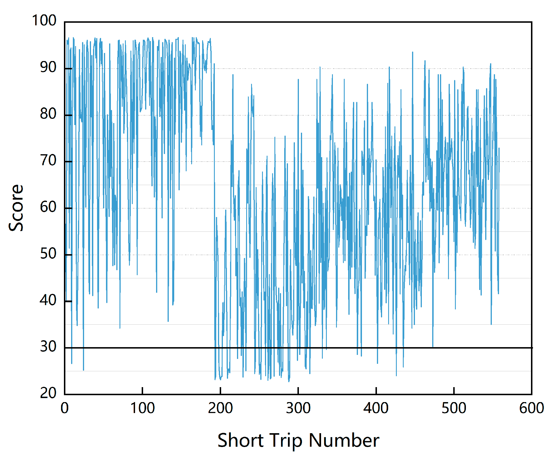
Figure 8 and Figure 9 are scores of the corresponding short trips in the two working conditions. In Figure 9 there is a significant increase in short trips with scores lower than 30, which is in line with Figure 7. Additionally, these low scores are concentrated in the smoother category of short trips. This category is the dominant type of short trip in weekend conditions and is a reflection of the better traffic environment on weekends. Therefore, it can be assumed that drivers in this environment are more likely to conduct extreme driving behaviors. In addition, the standard deviation of the scores for smoother short trips is 18.76, which is 37% higher than that for smooth ones (13.65). It is implied that there is more randomness in the traffic environment on weekends than in the more regular traffic flow on weekdays, thus drivers have to improvise all the time, causing large fluctuations in vehicle economy.

The analysis of driving behavior economy scores leads to the following conclusions:

• The increase in the proportion of aggressive driving behavior in weekend working conditions is caused by the superior traffic environment.
• The increased randomness of driving behavior in weekend working conditions has an impact on vehicle economy and needs to be further explored.

6. Conclusions

This study proposes a new way of constructing working conditions and verifies the validity and accuracy of the approach. On this basis, the driving behavior economy under the two constructed working conditions are quantitatively analyzed. The obtained score further confirms that the two different working conditions have different impacts on the driver. The main conclusions are as follows:

• The proposed method constructs two working conditions which regularly change in time to represent a new standpoint, thus providing new options for researchers and vehicle companies to conduct relevant studies and launch bus tests.
• During the vehicle design stage or in-vehicle software development, it is possible and easier to preset the running logic to reduce the negative impact brought about by the aggressive driving behavior on the bus economy because it only needs date identification.
• Since drivers may generate different emotions under the two constructed working conditions, it is necessary for personnel managers to control the driver’s psychological situation by establishing some regulations for rewards and penalties, which should be different on weekdays from those on weekends. In this way the economy of the bus could be improved to an extent.

This study only provides a preliminary quantitative analysis of the driver’s driving behavior economy. Future work includes in-depth analysis of more multidimensional and larger amounts of driving data as well as more complex and comprehensive working conditions. More routes and buses will be considered to obtain a more sufficient accuracy for the two constructed working conditions as well as to compare the different driving performances of more drivers. Meanwhile, instead of just using the PCA and k-means clustering method, some optimization algorithms are under evaluation to help construct working conditions and better evaluate the driving behavior economy.

References

- Kivekas, K.; Vepsalainen, J.; Tammi, K. Stochastic Driving Cycle Synthesis for Analyzing the Energy Consumption of a Battery Electric Bus. IEEE Access 2018, 6, 55586–55598. [Google Scholar] [CrossRef]
- Nan, S.R.; Tu, R.; Li, T.Z.; Sun, J.; Chen, H.B. From driving behavior to energy consumption: A novel method to predict the energy consumption of electric bus. Energy 2022, 261, 125188. [Google Scholar] [CrossRef]
- Nesamani, K.S.; Subramanian, K.P. Development of a driving cycle for intra-city buses in Chennai, India. Atmos. Environ. 2011, 45, 5469–5476. [Google Scholar] [CrossRef]
- Lin, J.; Niemeier, D.A. Regional driving characteristics, regional driving cycles. Transp. Res. D Transp. Environ. 2003, 8, 361–381. [Google Scholar] [CrossRef]
- Qiu, H.X.; Cui, S.Z.; Wang, S.T.; Wang, Y.Z.; Feng, M.L. A Clustering-Based Optimization Method for the Driving Cycle Construction: A Case Study in Fuzhou and Putian, China. IEEE Trans. Intell. Transp. Syst. 2022, 23, 18681–18694. [Google Scholar] [CrossRef]
- Ashtari, A.; Bibeau, E.; Shahidinejad, S. Using Large Driving Record Samples and a Stochastic Approach for Real-World Driving Cycle Construction: Winnipeg Driving Cycle. Transp. Sci. 2014, 48, 170–183. [Google Scholar] [CrossRef]
- Xie, S.B.; Zhang, S.Y.; Shi, S.S.; Wang, H.Q. Impact Analysis of Typical Driving Cycle Construction Methods for Energy Consumption of New Energy Vehicles. China J. Highw. Transp. 2022, 35, 361–371. [Google Scholar] [CrossRef]
- Perhinschi, M.G.; Marlowe, C.; Tamayo, S.; Tu, J.; Wayne, W.S. Evolutionary Algorithm for Vehicle Driving Cycle Generation. J. Air Waste Manag. Assoc. 2011, 61, 923–931. [Google Scholar] [CrossRef]
- Meixia, J.; Jianjun, H.; Haitao, L. Analysis and formulation of general running cycle of light vehicles. In Proceedings of the AIAM2021: 2021 3rd International Conference on Artificial Intelligence and Advanced Manufacture, New York, NY, USA, 23–25 October 2021; pp. 2384–2389. [Google Scholar] [CrossRef]
- Hao, Y.Z.; Zhang, J.; Wang, S.C.; Qiu, Z.W. Construction of Typical Driving Cycle for Public Buses in Wuhan City. J. Transp. Inf. Saf. 2014, 32, 139–145. [Google Scholar]
- Steinhauser, K.; Leist, F.; Maier, K.; Michel, V.; Parsch, N.; Rigley, P.; Wurm, F.; Steinhauser, M. Effects of emotions on driving behavior. Transp. Res. Part F Traffic Psychol. Behav. 2018, 59, 150–163. [Google Scholar] [CrossRef]
- Zhang, Y.; Guo, Z.; Sun, Z. Influencing Factors of Aggressive Driving Behavior in Driving Simulation Environment. China J. Highw. Transp. 2020, 33, 129–136. [Google Scholar]
- Hou, H.J.; Jin, L.S.; Guan, Z.W.; Du, H.X.; Li, J.J. Effects of Driving Style on Driver Behavior. China J. Highw. Transp. 2018, 31, 18–27. [Google Scholar]
- Zhang, H.N. Energy Consumption Law and Energy-Saving Measures Based on Driving Behavior. Ph.D. Thesis, Chang’an University, Xi’an, China, 2020. [Google Scholar]
- Tu, R.; Xu, J.S.; Li, T.Z.; Chen, H.B. Effective and Acceptable Eco-Driving Guidance for Human-Driving Vehicles: A Review. Int. J. Environ. Res. Public Health 2022, 19, 7310. [Google Scholar] [CrossRef]
- Sullman, M.J.M.; Dorn, L.; Niemi, P. Eco-driving training of professional bus drivers—Does it work? Transp. Res. Part C Emerg. Technol. 2015, 58, 749–759. [Google Scholar] [CrossRef]
- Kim, K.; Park, J.; Lee, J. Fuel Economy Improvement of Urban Buses with Development of an Eco-Drive Scoring Algorithm Using Machine Learning. Energies 2021, 14, 4471. [Google Scholar] [CrossRef]
- Andrieu, C.; Saint Pierre, G. Using statistical models to characterize eco-driving style with an aggregated indicator. In Proceedings of the 2012 IEEE Intelligent Vehicles Symposium (IV), Alcala de Henares, Madrid, Spain, 3–7 June 2012; pp. 63–74. [Google Scholar]
- Zhou, Y.W.; Guo, F.X.; Wu, S.M.; He, W.Y.; Xiong, X.F.; Chen, Z.; Ni, D.A. Safety and Economic Evaluations of Electric Public Buses Based on Driving Behavior. Sustainability 2022, 14, 772. [Google Scholar] [CrossRef]
- Jachimczyk, B.; Dziak, D.; Czapla, J.; Damps, P.; Kulesza, W.J. IoT On-Board System for Driving Style Assessment. Sensors 2018, 18, 1233. [Google Scholar] [CrossRef]
- Fugiglando, U.; Massaro, E.; Santi, P.; Milardo, S.; Abida, K.; Stahlmann, R.; Netter, F.; Ratti, C. Driving Behavior Analysis through CAN Bus Data in an Uncontrolled Environment. IEEE Trans. Intell. Transp. Syst. 2019, 20, 737–748. [Google Scholar] [CrossRef]
- Zhang, J.; Wang, Z.P.; Liu, P.; Zhang, Z.S.; Li, X.Y.; Qu, C.H. Driving cycles construction for electric vehicles considering road environment: A case study in Beijing. Appl. Energy 2019, 253, 14. [Google Scholar] [CrossRef]
- Jolliffe, I.T.; Cadima, J. Principal component analysis: A review and recent developments. Philos. Trans. R. Soc. A-Math. Phys. Eng. Sci. 2016, 374, 16. [Google Scholar] [CrossRef]
- Jain, A.K. Data clustering: 50 years beyond K-means. Pattern Recognit. Lett. 2010, 31, 651–666. [Google Scholar] [CrossRef]
- Ismkhan, H. I-k-means- plus: An iterative clustering algorithm based on an enhanced version of the k-means. Pattern Recognit. 2018, 79, 402–413. [Google Scholar] [CrossRef]
- Diakoulaki, D.; Mavrotas, G.; Papayannakis, L. Determining objective weights in multiple criteria problems: The CRITIC method. Comput. Oper. Res. 1995, 22, 763–770. [Google Scholar] [CrossRef]
- Tan, W.W.; Yan, Q.Y.; Gu, J.J.; Li, W.; Ji, X.F. Driving Style Recognition and Quantification for Heavy-duty Truck Drivers. J. Transp. Syst. Eng. Inf. Technol. 2022, 22, 137–148. [Google Scholar] [CrossRef]
Figure 1.
Pure electric bus operating route. (A) Nanhu terminal; (B) Tianhe terminal.
Figure 2.
An example of a short trip.
Figure 3.
Mean feature parameter values of 3 short trip categories (weekday).
Figure 4.
Mean feature parameter values of 2 short trip categories(weekend).
Figure 5.
Weekday working condition (2015s).
Figure 6.
Weekend working condition (2079s).
Figure 7.
Score comparison.
Figure 8.
Weekday trip scores.
Figure 9.
Weekend trip scores.