Article

Modelling and Dynamic Analysis of Adaptive Neuro-Fuzzy Inference System-Based Intelligent Control Suspension System for Passenger Rail Vehicles Using Magnetorheological Damper for Improving Ride Index

1
School of Engineering & Applied Science, Gati Shakti Vishwavidyalaya, Vadodara 390004, India
2
Mechanical Engineering Department, Graphic Era (Deemed to be University), Dehradun 248002, India
3
Department of Smart Manufacturing Engineering, Changwon National University, Changwon 51140, Republic of Korea
4
School of Mechanical Engineering, Changwon National University, Changwon 51140, Republic of Korea
*
Author to whom correspondence should be addressed.
Sustainability 2023, 15(16), 12529; https://0-doi-org.brum.beds.ac.uk/10.3390/su151612529
Submission received: 14 May 2023 / Revised: 10 August 2023 / Accepted: 15 August 2023 / Published: 18 August 2023
(This article belongs to the Special Issue Sustainable Railway Infrastructure and Rolling Stock)

Abstract

:
The ride comfort and safety of passenger rail vehicles depend on the performance of the suspension system in attenuating vibrations induced by track irregularities. This paper investigates the effectiveness of an Adaptive Neuro-Fuzzy Inference System (ANFIS)-based semi-active controlled suspension system using a magnetorheological fluid damper in reducing nonlinear lateral vibrations of a passenger rail vehicle. A complete rail vehicle model is developed, including the carbody, front and rear bogies, and the passive suspension system’s nonlinear stiffness and damping characteristics are considered from experimental data. The passive suspension model is validated through experiments, and an ANFIS-based controller is incorporated with the secondary vertical suspension system to improve ride behavior. Three semi-active suspension strategies are considered under varying speeds and track irregularities, and their effectiveness is compared to the nonlinear passive suspension system in terms of rms acceleration, rms displacement, ride quality, and comfort. The results shows that the ANFIS-based semi-active suspension system with a magnetorheological fluid damper outperforms the passive suspension system and semi-active strategies in all tested conditions. There is a reduction in rms acceleration by approximately 11.11% to 23.64% and rms displacement by about 5.36% to 32.06%. Moreover, it significantly improves ride quality (9.20% to 31.02%) and comfort (9.96% to 31.50%). The rms acceleration and displacement are reduced, and the Sperling ride index and Percentage Reduction Index values demonstrate that the ANFIS-based semi-active suspension effectively minimizes the impact of rail irregularities and vibrations, resulting in a significant gain in ride quality and passenger comfort.

1. Introduction

The field of railway transportation has seen significant advancements over the years, with a primary focus on enhancing passenger comfort, safety, and overall ride quality. The suspension system of passenger rail vehicles plays a crucial role in mitigating vibrations induced by track irregularities, thereby influencing ride comfort and safety. While providing some level of vibration attenuation, traditional passive suspension systems often fall short in handling the complexities of the nonlinear lateral vibrations that arise from varying track conditions [1].
Research in this area is primarily focused on understanding the fundamental dynamics of rail vehicles and their interaction with the track. These studies laid the groundwork for analyzing the effects of track irregularities on ride quality and passenger comfort. Researchers such as Jafari and Mashadi [2] explored the relationship between vehicle dynamics and ride comfort, highlighting the importance of suspension design in minimizing vibrations induced by track irregularities. The limitations of passive suspension systems spurred the development of semi-active and active control strategies. Semi-active suspension systems, in particular, garnered attention due to their potential to adapt to changing conditions while avoiding the complexity and energy consumption associated with fully active systems. Researchers like Cebon and Wong focused on semi-active control methods, investigating how controlled dampers can improve ride quality and safety [3,4].
In recent years, the integration of intelligent control systems into railway suspension has garnered significant attention. This interest stems from their potential to overcome the limitations of conventional systems and provide improved performance. Among these advanced approaches, the Adaptive Neuro-Fuzzy Inference System (ANFIS) has emerged as a particularly promising method for devising control strategies that can seamlessly adapt to changing conditions while enhancing the dynamic behavior of rail vehicles. Semi-active control methods, when combined with state-of-the-art suspension components like magnetorheological (MR) dampers, have demonstrated substantial promise in achieving exceptional vibration isolation and elevated ride quality indices [1]. Undoubtedly, the suspension system of passenger rail vehicles stands as a critical element, exerting direct influence over passenger comfort, ride quality, and overall safety. Although traditional passive suspension systems have proven effective to a certain extent, they often struggle to deliver optimal performance under dynamically changing conditions.
In response to these challenges, dedicated researchers in the field of railway transportation have invested substantial effort to elevate the performance of rail vehicle suspension systems. In recent years, intelligent control strategies have emerged as a promising avenue [5,6]. The ANFIS technique has garnered attention due to its hybrid nature, combining the strengths of fuzzy logic and neural networks. This hybrid capability endows ANFIS with the ability to effectively capture nonlinear relationships [7,8,9]. Various engineering applications have demonstrated the efficacy of ANFIS, and researchers such as Boada et al. [10] have harnessed techniques like recursive lazy learning based on neural networks to model the behavior of MR dampers in the context of railway transportation. This approach streamlines the modeling process and employs sample inputs to guide decision making. Arias et al. [11], on the other hand, opted for a second-order polynomial model to characterize MR damper behavior, leveraging the results to devise and implement a semi-active control algorithm.
Dimock et al. [12] chose to employ Bingham’s biplastic analysis to calculate the shear thinning and shear thickening properties of magnetorheological fluids. Additionally, Sharma and Sharma [13] proposed an adapted Bingham model that accurately reproduces the hysteresis behavior of MR dampers. Meanwhile, Fang. Y.Y [14] developed a neural network model featuring 6 input neurons, 1 output neuron, and 12 neurons within a hidden layer, effectively emulating the dynamic behavior of MR dampers. Empirical studies and mathematical modeling on MR dampers were conducted by Maharani et al. [15] and Han et al. [16], contributing valuable insights to the field. Altogether, these efforts underscore the continuous strides being made to enhance railway suspension systems through innovative intelligent control strategies and advanced modeling techniques.
This paper addresses a substantial research gap by evaluating the efficacy of an ANFIS-based semi-active suspension system to enhance the operational performance of high-speed trains. The primary focus of this investigation lies in the attenuation of lateral vibrations in passenger rail vehicles stemming from track irregularities. The research methodology encompasses the development of a comprehensive rail vehicle model, which incorporates experimentally derived nonlinear suspension characteristics. The methodology involves the integration of an ANFIS-based semi-active controlled magnetorheological damper into the vertical suspension system architecture. This integration elevates ride quality and enhances passenger comfort through adaptive vibration mitigation. The ANFIS methodology, which harmonizes fuzzy logic and neural networks, is systematically contrasted against alternative controllers for semi-active rail vehicle suspension. The empirical results unequivocally underscore the ANFIS approach’s superiority in its ability to mitigate vibrations and enhance passenger comfort effectively.
This paper makes a significant contribution to the field of rail vehicle suspension systems by focusing on the improvement of ride comfort and safety through the utilization of an ANFIS-based semi-active controlled suspension system integrated with magnetorheological (MR) dampers. The research presents a comprehensive investigation that combines theoretical modelling and practical experimentation. By developing a detailed rail vehicle model, incorporating nonlinear elements and track irregularities and accurately capturing the dynamic behavior of MR dampers, the paper offers insights into the complex interactions within rail vehicle suspension systems. The proposed ANFIS-based control strategy demonstrates superior adaptability and effectiveness in attenuating vibrations induced by track irregularities. The achieved reduction in RMS acceleration and displacement, coupled with improved ride indices, showcases the practical applicability of the approach. The research provides a novel method for enhancing passenger comfort and ride quality and establishes the superiority of the ANFIS-based controller over other strategies. This work’s contribution extends to the broader rail vehicle suspension design context and lays the foundation for more advanced and adaptive semi-active control solutions, enhancing rail transportation systems’ overall passenger experience and safety.

2. Materials and Methods

The mathematical modelling of a nonlinear rail vehicle involves developing equations of motion that accurately describe how the carbody, bogie frames, and wheel axle respond to various forces and motions. The model includes four vertical dampers that form the primary suspension and two vertical dampers, one lateral damper, and two yaw dampers to create the secondary suspension, all considered nonlinear elements [17,18]. To construct the equations of motion, the behavior of the rail vehicle is analyzed in four distinct directions: vertical (up and down motion), lateral (side-to-side motion), yaw (rotation along its vertical axis), and roll (rotation along its longitudinal axis), as depicted in Figure 1.
The primary suspension comprises four vertical dampers that absorb and counteract the vertical forces acting on the carbody. Conversely, the secondary suspension utilizes the combination of two dampers on the vertical, one damper on the lateral side, and two dampers on the yaw side to mitigate forces and motions occurring in the lateral, yaw, and roll directions. Consequently, the equations of motion for the carbody, bogie frames, and wheel axle are formulated, encompassing information about the vehicle’s displacement, velocity, and acceleration in each of the mentioned directions. These equations are inherently nonlinear due to integrating the spring and damper as nonlinear elements.

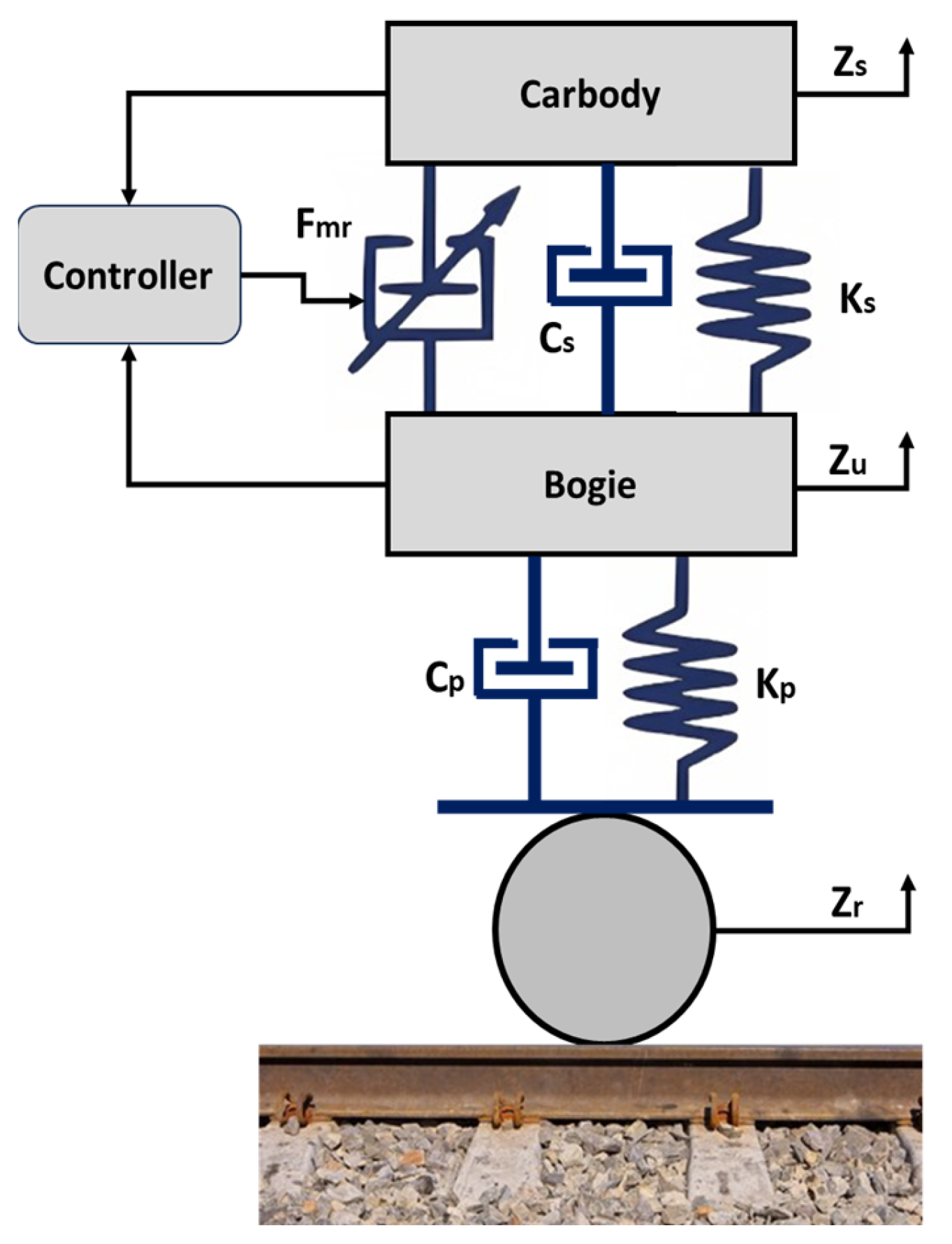
2.1. EoM of Rail Vehicle Model

The equations of motion (EoM) for the formulated rail vehicle model travelling on a straight track are expressed as follows:

2.1.1. Nonlinear Elements in Rail Vehicle

The mathematical modelling of a rail vehicle includes both primary and secondary suspension systems, with various nonlinear elements considered. These nonlinear elements consist of springs and dampers that exhibit nonlinear force-displacement and force-velocity characteristics. These elements are crucial for absorbing and countering forces and vibrations that arise from track irregularities and train speed. The primary suspension system incorporates four primary vertical springs (kpz) and four primary vertical dampers (cpz). On the other hand, the secondary suspension system is composed of two secondary vertical springs (ksz), two secondary vertical dampers (csz), one secondary lateral damper (csy), and two secondary yaw dampers (csy). The force-displacement relationship for the primary vertical spring (fpzk) is described by Equation (1), while the force-displacement relationship for the secondary vertical spring (fszk) is represented by Equation (2). Additionally, the force-velocity characteristics of the dampers are given by Equations (3)–(6) for the primary vertical damper (fpzd), secondary vertical damper (fszd), secondary lateral damper (fsyd), and secondary yaw damper (fsxd). Xwbz, xbcz are the relative displacement between wheel-bogie and bogie-carbody, respectively. x ˙ w b z , x ˙ b c z , x ˙ b c y , x ˙ b c x are the relative velocity (vertical) between wheel-bogie, bogie-carbody, lateral bogie-carbody, yaw bogie-carbody, respectively. Forcemax is the maximum force of the respective damper.
f p z k = a 1 exp ( a 2 x w b z ) + a 3 x w b z 2
f s z k = b 1 exp ( b 2 x b c z ) + b 3 x b c z 2
f p z d = F o r c e max p z d sin g p z d x ˙ w b z + h p z d
f s z d = F o r c e max s z d sin g s z d x ˙ b c z + h s z d
f s y d = F o r c e max s y d sin g s y d x ˙ b c y + h s y d
f s z d = F o r c e max s z d tanh g s z d x ˙ b c x + h s z d
The constant parameters used in the equations are derived from experimental data, and their values are provided in Table 1. These values are obtained through nonlinear least-square optimization using MATLAB(R2022a) software.
Figure 2 and Figure 3 illustrate the force-relative displacement characteristics for the vertical suspension stiffness (both primary and secondary) and the damping force-relative velocity characteristics of the dampers (primary vertical, secondary vertical, secondary lateral, and secondary yaw).

2.1.2. EoM of Carbody

The Equations (7)–(10) are the EoM for the carbody mass center of a vehicle. In these equations, the subscript i indicates which direction of motion is being considered (i.e., vertical (z), lateral (y), yaw (ψ), or roll (ϕ)). The various parameters defined as the carbody have a mass of 5.05 × 10⁴ kg, and its mass moment of inertia is 5.69 × 10⁴ kg m2 for roll (Icx), 1.307 × 10⁶ kg m2 for pitch (Iyc), and 1.309 × 10⁶ kg m2; for yaw (Izc). The bogie, on the other hand, weighs 2.41 × 10³ kg, and its mass moment of inertia is 2.159 × 10³ kg m2 for roll (Ibx), 1.389 × 10³ kg m2 for pitch (Iby), and 3.387 × 10³ kg m2 for the overall frame (Ibz). The center pin spacing of the half bogie (L) is 7.45 m, the half distance of the wheelbase (D) is 1.280 m, half of the primary suspension lateral spacing (go) is 1 m, and half of the wheelset contact distance (a) is 0.8380 m. Half of the secondary suspension lateral spacing (eh) is 1 m. The distances of the center of gravity for both the bogie frame and the carbody to the secondary suspension in the vertical direction are provided as 0.2170 m (pts) and 1.36 m (pcs), respectively. Moreover, the distance from the bogie frame’s center of gravity to the primary suspension in the vertical direction is specified as −0.4520 m (ptp), and the distance from the wheelset’s center of gravity to the primary suspension in the vertical direction is 0.1800 m (pwp). Vertical wheelset disturbance of 1–4 right (z1r, z2r, z3r, z4r) and left (z1l, z2l, z3l, z4r).
m c Z c ¨ = 2   Force   max s z d sin g s z d z ˙ r b + z ˙ f b 2 z ˙ c + h s z d + 2 b 1 exp b 2 z r b + z f b 2 z c + b 3 z r b + z f b 2 z c 2
m c y ¨ c = 2   Force     max s y d sin g s y d y ˙ r b y ˙ f b + 2 y ˙ c + 2 h c h T   ϕ ˙ c + h s y d
I c x ϕ ¨ c = 2 b 1 e x p b 2 b 2   2 ϕ f b + b 2   2 ϕ r b 2 b 2   2 ϕ c + b 3 b 2   2 ϕ f b + b 2   2 ϕ r b 2 b 2   2 ϕ c 2 + 2   Force     m a x s z d s i n g s z d b 3 2 ϕ ˙ t 1 + b 3 2 ϕ ˙ t 2 2 b 3 2 ϕ ˙ c + h s z d 2   Force     m a x s y d s i n g s y d 2 h c h T y ˙ c h c h T y ˙ t 2 h c h T y ˙ t 1 + 2 h c h T 2 ϕ ˙ c + h s y d
I c z ψ ¨ c = 4 L c 2   Force     max s y d sin g s y d ψ ˙ c + h s y d 2 L c   Force     max s y d sin g s y d y ˙ t 1 + y ˙ t 2 + h s y d 2 b 3 2   Force     max s x d tan h g s z d 2 ψ ˙ c ψ ˙ f b ψ ˙ r b + h s z d

2.1.3. EoM of Bogie Frame

The Equations (11)–(14) are the EoM for a vehicle’s front and rear bogie frames. In these equations, the subscript i indicates which bogie frame (i.e., front or rear). In contrast, the subscript j indicates which direction of motion is considered (i.e., vertical, lateral, yaw, or roll).
m b z ¨ i b = 2 ( a 1 e x p a 2 2 z i b + z i b w 1 + z i b w 2 + a 3 2 z i b + z i b w 1 + z i b w 2 2 ) 2 b 1 exp b 2 z i b + b 3 z i b 2   + 2   Force     m a x p z d s i n g p z d 2 z ˙ i b + z ˙ i b w 1 + z ˙ i b w 2 + h p z d 2   Force     m a x s z d sin g s z d z ˙ i b + h s z d
m b y ¨ i b = K p y 2 y i b w 1 + 2 y i b w 2 4 y i b 4 h T ϕ i b F o r c e m a x s y d s i n ( g s s d ( 2 y ˙ f b 2 ( 1 ) i L c ψ ˙ c 2 y ˙ c 2 h c h T ϕ ˙ c ) + h s s d )
I b x ϕ ¨ i b = 2 b 1 e x p b 2 b 2 2 ϕ i b b 2 2 ϕ c + b 3 b 2 2 ϕ c b 2 2 ϕ i b 2 + 2   Force     m a x s z d s i n g s z d b 3 2 ϕ c ˙ b 3 2 ϕ ˙ i b + h s z d 2 a 1 e x p a 2 2 b 1 2 ϕ i b b 1 2 ϕ i b w 1 b 1 2 ϕ i b w 2 + a 3 x w b z 2 2   Force     m a x p z d s i n g p z d 2 b 1 2 ϕ ˙ i b b 1 ϕ ˙ i b w 1 b 1 2 ϕ ˙ i b w 2 + h p z d
I b z ψ ¨ i b = 2 F o r c e e m a x s x d t a n h ( g s x d ( b 3 2 ψ ˙ i b b 3 2 ψ ˙ c ) + h s x d )

2.1.4. EoM of Wheel Axle

The Equations (15)–(18) are the EoM for a vehicle’s front and rear wheel axles. In these equations, the subscript i indicates which axle (i.e., front or rear), while the subscript j indicates which direction of motion is considered (i.e., vertical, lateral, yaw, or roll). { i = f while j = 1 2 , i = r while j = 3 4 } .
m w y ¨ w i j = 2 α i j f 11 V V ψ w i j y ˙ w i j W e x t + m w g ϕ w i j 2 r 0 α i j f 11 V ϕ ˙ w i j 2 α i j f 12 V ψ ˙ w i j V R W e x t + m w g ϕ s e + V 2 W e x t g R + 2 K p y y w i j ( ) j 2 K p y L 1 ψ i b + 2 K p y y i b 2 C p y y ˙ w i j ( 1 ) j 2 C p y L 2 ψ ˙ i b + 2 K p y h T ϕ i b + 2 C p y y ˙ i b + 2 C p y h T ϕ ˙ i b
m w z ¨ w i j = 2 f 11 V y ˙ w i j ϕ w i j + 2 f 12 R ϕ w i j 2 λ 2 f 11 V y w i j ϕ ˙ w i j 2 f 12 V ϕ w i j ψ ˙ w i j 2 r 0 f 11 V ϕ w i j ϕ ˙ w i j + 2 λ 2 f 12 r 0 + 2 a 1 e x p ( a 2 z i b z w i j ) + a 3 z i b z w i j 2 + 2 F o r c e m a x p = d s i n g p z d z ˙ i b z ˙ w i j + h p z d
I w x ϕ ¨ w i j = I w y V r 0 ψ ˙ w i j V R 2 λ 2 α i j f 12 r 0 y w i j 2 r 0 f 11 V a λ + α i j r 0 ϕ ˙ w i j + 2 λ 2 f 12 + 2 a λ f 12 r 0 1 α i j ϕ w i j 2 f 12 a λ + α i j r 0 v y ˙ w i j W e x t + m w g + V 2 W e x t g R ϕ s e λ 2 y w i j + W e x t + m w g + V 2 W e x t g R ϕ s e × a λ ϕ w i j + 2 f 11 a λ + α i j r 0 + 2 f 22 λ 2 r 0 ψ w i j + 2 f 12 R a λ + α i j r 0 2 f 12 V a λ + α i j r 0 ψ ˙ w i j + 2 a 1 e x p a 2 b 1 2 ϕ i b b 1 2 ϕ w i j + a 3 b 1 2 ϕ i b b 1 2 ϕ w i j 2 + 2 F o r c e m a x p z d s i n g p z d b 1 2 ϕ ˙ i b b 1 2 ϕ ˙ w i j + h p z d + h W e x t V 2 g R ϕ s e ϕ w i j
I w x ψ ¨ w i j = 2 a λ α i j f 33 r 0 y w i j 2 a 2 α i j f 33 V + 2 α i j f 22 V ψ ˙ w i j 2 α i j f 12 ψ w i j + W e x t + m w g + V 2 W e x t g R ϕ s e a λ ψ w i j I w y V r 0 2 r 0 α i j f 12 V ( ϕ ˙ w i j ) + 2 α i j f 12 V + 2 α i j R a 2 f 33 + f 22 2 C p x b 1 2 ψ ˙ w i j + 2 K p x b 1 2 ψ i b 2 K p x b 1 2 ψ w i j + 2 C p x b 1 2 ψ ˙ i b

2.2. Modelling of Track Irregularities

The track irregularity is a significant factor in railway vehicles’ dynamic behavior and ride comfort. The model under consideration utilizes sinusoidal rail irregularities as inputs for the inner and outer rail surfaces [8,19,20]. The scalar factor A and spatial frequency Ω represent these irregularities and are expressed in Equation (19). Specifically, the irregularity incorporates three harmonics and has a spatial length of 25 m. The front wheelset of the front bogie is subjected to vertical excitation represented by z1l and z1r.
Z 1 r t Z 1 l t = 4 A π 1 3 c o s Ω x 1 15 c o s 2 Ω x + 1 35 c o s 3 Ω x 4 A π 1 3 c o s Ω x 1 15 c o s 2 Ω x + 1 35 c o s 3 Ω x
Furthermore, the vertical excitations of other wheel axles, namely z2r, z3r, and z4r for right wheels, and z2l, z3l, and z4l for left wheels, have the time lags τ1, τ2, and τ3, respectively, as presented in Equation (20). The time delays are calculated based on the distance between the wheelsets and the vehicle speed. These time delays are vital because they represent the time required for the rail irregularities to propagate from the front wheelset to the other wheelsets.
Z 2 r t Z 2 l t = Z 1 r t τ 1 Z 1 l t τ 1 ; Z 3 r t Z 3 l t = Z 1 r t τ 2 Z 1 l t τ 2 ; Z 4 r t Z 4 l t = Z 1 r t τ 3 Z 1 l t τ 3
The proposed model considers three harmonics of the track irregularities, which are known to significantly impact the dynamic behavior of railway vehicles. The scalar factor A and spatial frequency Ω are used to characterize the amplitude and frequency of the irregularities, respectively. Using sinusoidal rail irregularities as inputs in the model allows for the simulation.

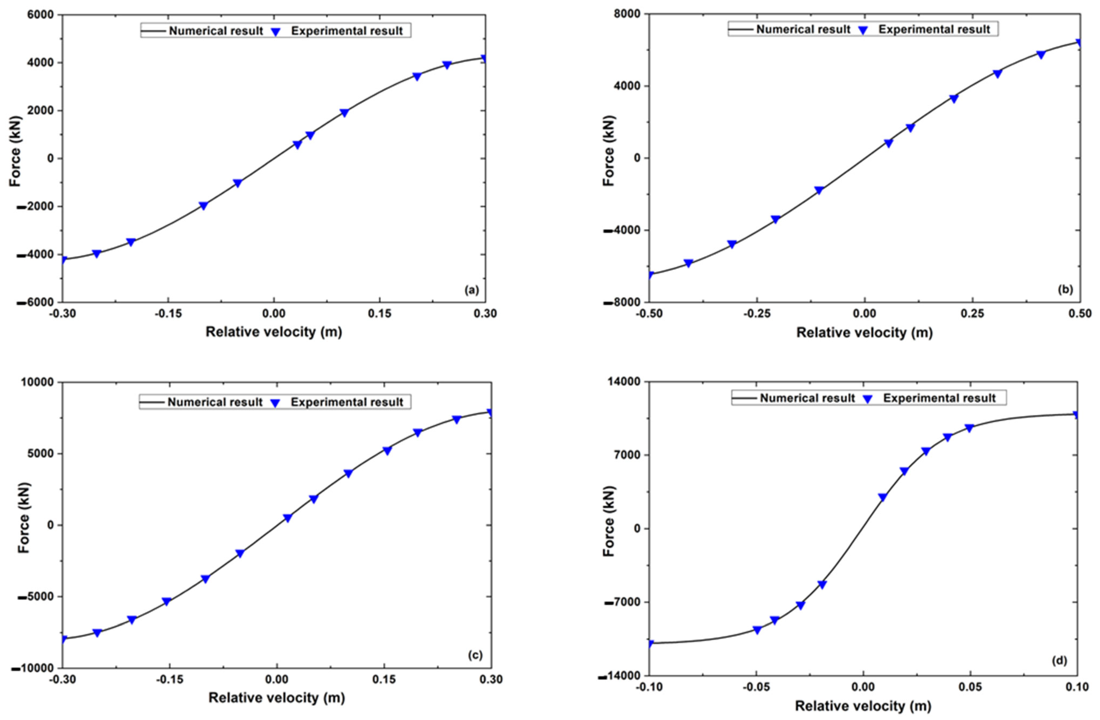
2.3. Mathematical Model of Magnetorheological (MR) Damper

2.3.1. Dynamic Model of MR Damper

A magnetorheological (MR) damper is a hydraulic shock absorber that utilizes a magnetically sensitive fluid to adjust its resistance and provide variable damping forces in response to the motion of a mechanical system.
A modified MR damper includes additional features, such as a bypass valve or external accumulator, to enhance its performance [21]. The dynamic behavior of MR damper force can be investigated using Equation (21). Figure 4 depicts a mechanical representation of an MR damper, which is an idealization based on the Bouc–Wen hysteresis model. This model effectively captures the behavior of the damper across a broad spectrum of input conditions.
It is regulated by the simultaneous Equations (21)–(25).
F d = c 1 y ˙ + k 1 x x 0
z ˙ = γ x ˙ y ˙ z z | n 1 β x ˙ y ˙ z | n + A x ˙ y ˙
y ˙ = α z + c 0 x ˙ + k 0 x y / c 0 + c 1
The following is an expression of the parameters that rely on the voltage that is being applied:
c 0 = c 0 a + c 0 b u c 1 = c 1 a + c 1 b u α = α a + α b u
The first-order filter considers the dynamics throughout the MR damper arriving at rheological equilibrium.
u ˙ = η u v
v is the voltage of the current generator.

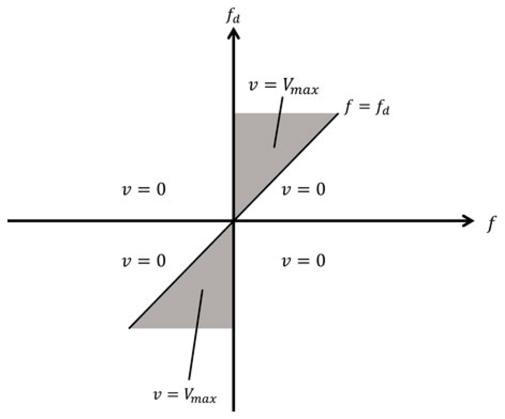
2.3.2. Control Algorithm for MR Damper

Controlling an MR damper with the use of acceleration feedback was the goal of Dyke’s 1996 [22] proposal for a clipped-optimal control approach, which is sometimes referred to as clipped voltage law. A clipped-optimal control strategy is used in control theory and engineering to ensure a system operates within a predefined set of constraints. In this strategy, the control inputs are clipped or limited to within a specific range or boundary, ensuring the system does not violate any constraints. The clipped-optimal control strategy can be formulated as an optimization problem that seeks to minimize a performance index subject to the constraints imposed on the system. The performance index typically identifies the control quality, such as errors between the system output and the desired setpoint. The constraint set may include physical constraints such as limits on the actuator inputs or the system’s operating conditions, or it could be a set of safety constraints that must be respected at all times to avoid catastrophic failures. The advantage of using a clipped-optimal control strategy is that it provides a systematic way to guarantee that the system remains safe and stable while achieving optimal control performance. It is advantageous in systems with hard physical constraints that cannot be violated. Hence, the clipped-optimal control strategy is a powerful tool for ensuring the safe and optimal control of dynamic systems subject to constraints, and its benefits and drawbacks must be carefully considered when applying it to a specific system. Providing a direct command to the force created in the MR damper is impossible. Direct control can only be exerted on the control voltage v supplied to the current driver. The formula that may describe the procedure for choosing the command signal for the MR damper is the following Equations (26) and (27).
v = V max H f d f f
v =   0 ,   for   f d < f V max ,   for   f d f f d × f 0
The desired optimal damping force (fd) is controlled based on the command voltage (v) and the maximum voltage (Vmax), employing a clipped-optimal control algorithm illustrated in Figure 5 [23].
The current driver increases the voltage to its maximum level to maintain a constant voltage applied to the MR damper when it produces the desired optimal force (f = fd). This increase aims to match the desired control force when the damper force magnitude is lower than the optimal force, and both forces have the same sign. Conversely, if the damper force magnitude differs or has a different sign than the desired force, the voltage applied to the damper is set to zero.
The analysis compares the performance of three MR damper modes: semi-active-low (Sa-L), semi-active-high (Sa-H), and semi-active control (Sa-C) mode. In the semi-active-low (Sa-L) mode, the damper is fixed at a low damping rate of 0.25 A. In the semi-active-high (Sa-H) mode, the damper is fixed at a high damping rate of 1 A when a certain vertical threshold velocity is reached. In the Sa-C mode, the damper continuously adjusts the damping rate in real-time based on sensor feedback. These modes are analyzed to assess their effectiveness in reducing vibrations and enhancing the system’s performance. Furthermore, the Percentage Reduction Index in Equation (28) is utilized to quantitatively compare various suspension strategies concerning the reduction in the root mean square (rms) amplitude (acceleration and displacement) of the carbody response and the improvement in ride indices.
P R I = P a s s i v e s e m i a c t i v e p a s s i v e × 100

2.4. Adaptive Neuro-Fuzzy Inference System (ANFIS)

ANFIS controllers combine fuzzy logic and neural networks to handle nonlinear aspects and adapt to changing conditions, resulting in enhanced control accuracy compared to traditional fuzzy controllers [24]. Hence, due to its universal approximation ability for nonlinear systems, the ANFIS method is used to build an MR damper model. The architecture of a two-input (x and y) and one-output (z) ANFIS is studied and shown in Figure 6. A common rule set with two fuzzy if-then rules is used for a first-order Sugeno fuzzy model, each defining a linear relationship between the inputs and outputs.
  • Rule 1: If x is A 1 , y is B 1 , then f 1 = p 1 x + q 1 y + r 1
  • Rule 2: If x is A 2 , y is B 2 , then f 2 = p 2 x + q 2 y + r 2
  • Rule N: If x is A n , y is B n , then f n = p n x + q n y + r n
Where x and y are model inputs and A 1 A n and B 1 B n are fuzzy sets. f 1 f n are the fuzzy outputs, and p i , q i , and r i are node parameters [24]. The fuzzy sets A1, A2, …, An and B1, B2, …, Bn can be defined using membership functions that assign membership degrees to the sets’ elements. The TSK (Takagi-Sugeno-Kang) fuzzy model is utilized, which is computationally efficient and well-suited for approximating nonlinear associations through piecewise linear relationships. This is particularly suitable for modelling the nonlinear behavior of an MR damper.
The layers are defined as follows:
Layer 1: Every node i in this layer is a square node with a note output.
Layer 2: Every node in this layer is a circle node labelled π, performing the T-norm operation by multiplying the incoming signals and outputting the result.
Layer 3: Every node in this layer is a circle node labelled N. The ith node calculates the ratio of the ith rule’s firing strength to the sum of all rules’ firing strengths
Layer 4: Every node i in this layer is a square node with a node function
Layer 5: The single node in this layer is labeled Ʃ, which computes the overall output as the summation of the incoming signals from the previous layer.

2.4.1. Fuzzy Identification of MR Damper

The fuzzy identification of the MR damper involves the following steps:
Collect sufficient training and checking data generated by the target model, including displacement, velocity, current signals, and corresponding force outputs from the MR damper. Utilize ANFIS to develop a fuzzy model that establishes the relationship between the input signals (displacement, velocity, and current) and the force produced by the MR damper. Validate the newly created fuzzy model by comparing its output to the output of the target model using the same inputs (displacement, velocity, and current signals). This validation ensures that the fuzzy model accurately represents the behavior of the MR damper under different conditions.

2.4.2. Data Collection

To develop the ANFIS setup, data for training and checking are obtained from the mathematical model of the MR damper proposed by Spencer et al. [4]. A 2-input type-3 ANFIS with 9 if-then rules is used to construct the fuzzy inference system (FIS). Each input is associated with three membership functions using the bell-shaped function in ANFIS. The training data are carefully selected to cover many damper operations. Displacements range from ±4 cm with a frequency content between 0 and 2 Hz, while current signals range from 0 to 3 A with frequencies up to 2 Hz. Gaussian white-noise band-limited signals are used for training, and MATLAB is used to solve the differential equations for a simulation time of 50 s with a time step of 0.001 s, resulting in 50,000 data sets. The training and checking data represent typical operational scenarios for the MR damper, including situations of maximum operational current and zero current.

2.4.3. Training of the Model

After establishing the training and checking data, ANFIS is employed to create a FIS that replicates the behavior of the MR damper. Before training the ANFIS, an initial blind FIS is constructed, meaning it has no prior knowledge of the target behavior. The FIS is designed with three inputs—displacement, velocity, and current—and a single output representing damping force. It is assumed that there is no time delay between the input and output signals. Velocity is obtained from the displacement signal using a second-order backward difference method. Out of the 50,000 original data sets, 25,000 are used for training, and the remaining 25,000 are used for checking the performance of the trained FIS.

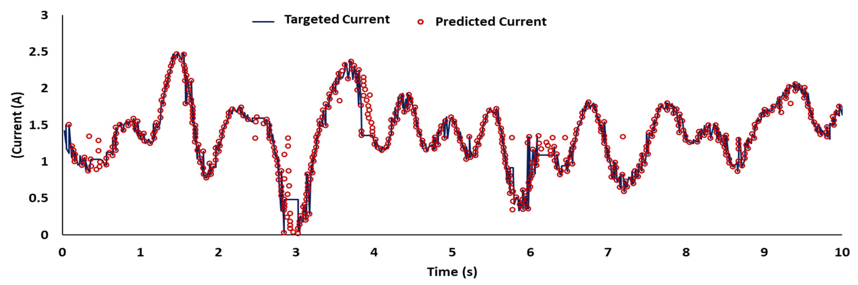
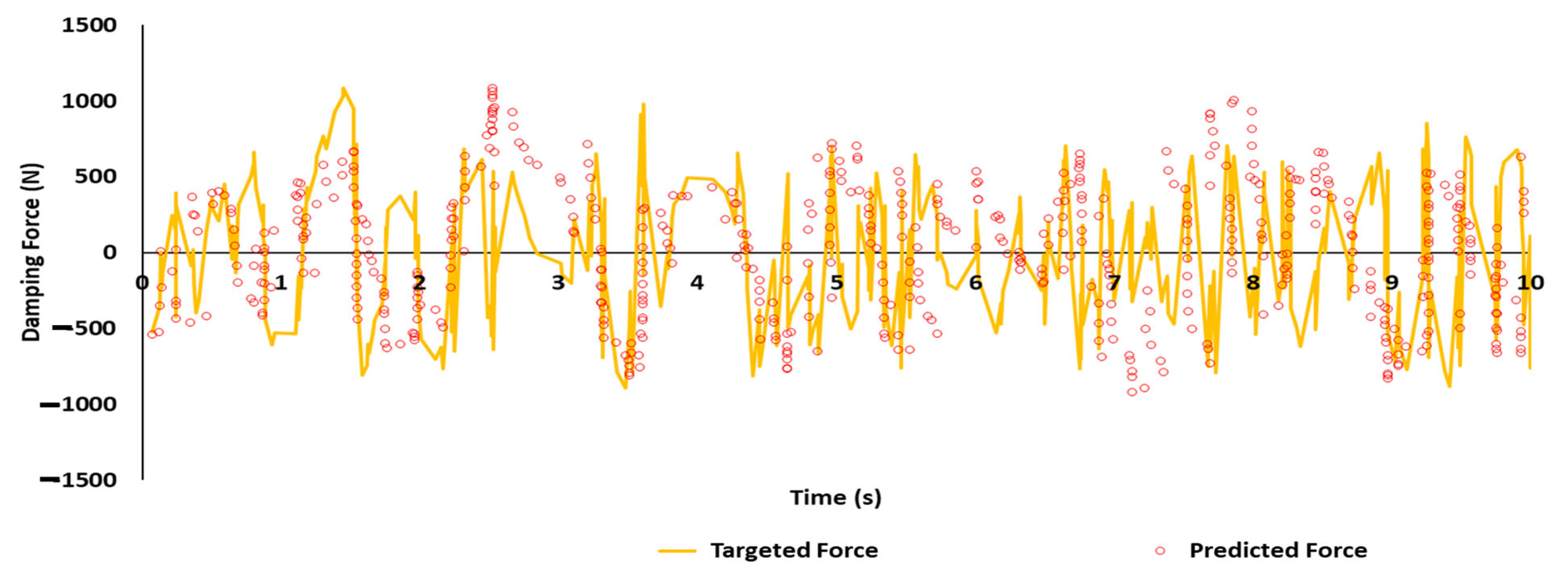
2.4.4. Model Validation

To validate the accuracy of the fuzzy model, a graphical and numerical comparison is made with the behavior of the mathematical model when subjected to identical inputs. Figure 7, Figure 8 and Figure 9 show the velocity of the piston across the MR damper, a comparison between the predicted current and target current, and a comparison between the predicted damping force and target damping force, respectively.
The process involves inputting the desired current and the piston conditions (displacement and velocity) into the mathematical model (a) to generate the target force. The predicted current obtained from the fuzzy model is then compared with the target current. Additionally, the target force is compared with the predicted force computed by the unified MR damper model (b), which has a different input current. As illustrated in Figure 9, the results indicate a close match between the predicted current and the damping force obtained from the ANFIS MR damper model and those of the mathematical model. The normalized errors between the predicted and model force in the time, displacement, and velocity domains can be accurately expressed in Equations (29)–(31), respectively. The close agreement between the predicted and model forces validates the accuracy and effectiveness of the ANFIS MR damper model in emulating the behavior of the mathematical model.
E t = 0 T F exp F 2 d x d t d t 0 T F exp μ exp 2 d x d t d t
E x = 0 T F exp F 2 d x d t d t 0 T F exp μ exp 2 d x d t d t
E x ˙ = 0 T F exp F 2 d x ˙ d t d t 0 T F exp μ exp 2 d x ˙ d t d t
In this equation, Fexp is the force predicted by the MR model, Ffuzzy represents the predicted force by fuzzy model, µexp is the mean of the force produced by the mathematical model over the duration T. Table 2 presents a collection of normalized errors.

3. Selection of ANFIS over Other Controllers for MR Damper Performance

Researchers have explored various control strategies to enhance suspension system performance. This investigation compares four controllers, PI, PID [25], fuzzy logic [26], and ANFIS [27], for the semi-active suspension system of a rail vehicle. The selection considered linear and nonlinear features, relevance, and appropriateness for the application. Linear controllers (PI and PID) provide a baseline for evaluation, while fuzzy logic handles imprecise or nonlinear behavior. ANFIS combines fuzzy logic and neural networks for adaptability and improved control accuracy. The analysis aims to identify the optimal control strategy for the rail vehicle’s suspension system, considering trade-offs between linear and nonlinear approaches. To analyze the performance of different suspension systems, two degrees of the rail vehicle system are considered (See Figure 10). Here, Z s and Z u are the vertical displacements of the carbody and bogie, respectively. The track input profile is denoted as Z r . The derivatives, i.e., the velocity and accelerations of the carbody and bogie masses, are represented by a single and double dot over the variables, respectively. k s is the secondary suspension spring’s stiffness and C s is the secondary suspension damper’s damping coefficient. The primary stiffness is represented by k p and the damping coefficient of the primary suspension system is C p . The MR damper force is given as F m r .
The mathematical model for comparing different controllers for analyzing the performance for the PSS can be obtained simply by removing the actuation force term from the following Equations (32) and (33).
M c Z ¨ c = C s Z ˙ s Z ˙ u k s Z s Z u + F a
  M b Z ¨ b = C s Z ˙ s Z ˙ u + k s Z s Z u C p Z ˙ u Z ˙ r k p Z u Z r F m r
The performance of suspension systems with different methods is tested with circular wave track bumps shown in Figure 11. The frequencies of these bumps are 0.1   Hz and 1   Hz . The circular wave of track irregularity is shown in Equation (34).
W x = a 1 u t 5 u t 10 sin 0.2 π t
where, a = 0.1   m   ( track bump height ) and c = 5   m (width).
The analysis of the performance of all the controllers has been presented in Figure 12. Additionally, Table 3 displays the ‘peak overshoot’ and ‘settling time’ at the front body velocity of the vehicle, specifically for a circular wave track input.
Figure 12 and Table 3 present the control system’s performance results. It is observed that the ANFIS controller outperforms the other control algorithms in terms of both “peak overshoot” and “settling time”. A decrease in the “peak overshoot” will reduce the vibrations experienced by the passenger. Reducing the “settling time” effectively minimizes the oscillations experienced in the carbody, enhancing passenger comfort to the highest degree. Therefore, this paper will consider the ANFIS controller to analyze a full-scale rail vehicle.

4. Numerical Validation of the Mathematical Model

A vibration test was conducted on the track to analyze the transition of vibrations between the primary and secondary suspension systems and the shaking between the vehicle body and the suspended equipment. Accelerometers and displacement sensors were employed to monitor accelerations at multiple locations on the carbody. The experiment was conducted on a specific section of the Indian railway track, specifically between Palwal and Mathura. The experimental data were then compared to a proposed numerical passive model for evaluating ride comfort. The oscillation tests were conducted using a prototype coach with sensors to accurately measure displacement, acceleration, events, and speed, as depicted in Figure 13. The passband frequency range for frame acceleration is 0.5 to 12 Hz, with a frame acceleration sampling frequency of 2 kHz. The acceleration measurement device has a passband frequency range of 0.1 to 200 Hz and a sampling frequency of 1 kHz. The maximum vertical and lateral ride indices were determined in unloaded and loaded states using different methodologies, specifically ORE C 116 and RDSO [28].
The riding behavior was considered for validation. A numerical simulation was conducted using the proposed model, considering the conditions of the RDSO test track for both empty and fully loaded cars. The results from the numerical analysis showed good agreement with the experimental data, validating the model’s accuracy. However, some differences in the riding index were observed, which could be attributed to factors not accounted for in the simplified mathematical model. Overall, the on-track vibration test and numerical simulation provide valuable insights into improving ride comfort for passengers. The comparison between the numerical and experimental analysis for empty and loaded carbodys is shown in Figure 14a,b.

5. Results

5.1. MR Damper Characteristics

A magnetorheological (MR) damper called the Bouc–Wen MR damper model is considered for the analysis. This model has constant parameters, meaning that the damper’s properties remain the same regardless of the operating conditions. This is a distinct advantage because the model can be effective for any preferred current level, frequency, and excitation amplitude set. Figure 15a–c is a graph that shows the hysteresis force of the Bouc–Wen MR damper versus time, displacement, and velocity. MATLAB SIMULINK, a piece of software that can be used to model and simulate dynamic systems, was used to create the graph. The findings achieved with an amplitude of 6.35 mm and a frequency of 10 Hz are shown in the graphs below using current excitations of 0.25 A, 0.75 A, and 1.25 A, respectively.
The response of Figure 15 shows that the hysteresis force exhibits distinctive patterns as the current excitation level varies. Higher current excitations generally correspond to increased damping performance, resulting in larger hysteresis loops. Moreover, while the frequency was constant during simulations, it is crucial to acknowledge its potential impact on the MR damper’s behavior. Frequencies outside the tested range may engender variations in the damper’s hysteresis loops, affecting its response to vibrations and disturbances. The analysis also sheds light on the time-varying nature of the MR damper’s response. This temporal adaptability is instrumental in comprehending the damper’s dynamic behavior within changing environments, thus enabling the design of control algorithms that capitalize on its real-time adaptability.

5.2. Acceleration and Displacement Response of Rail Vehicle

Acceleration and displacement responses are critical aspects in the design and analysis of vehicle suspension systems, as they directly influence ride comfort, handling, and overall safety.

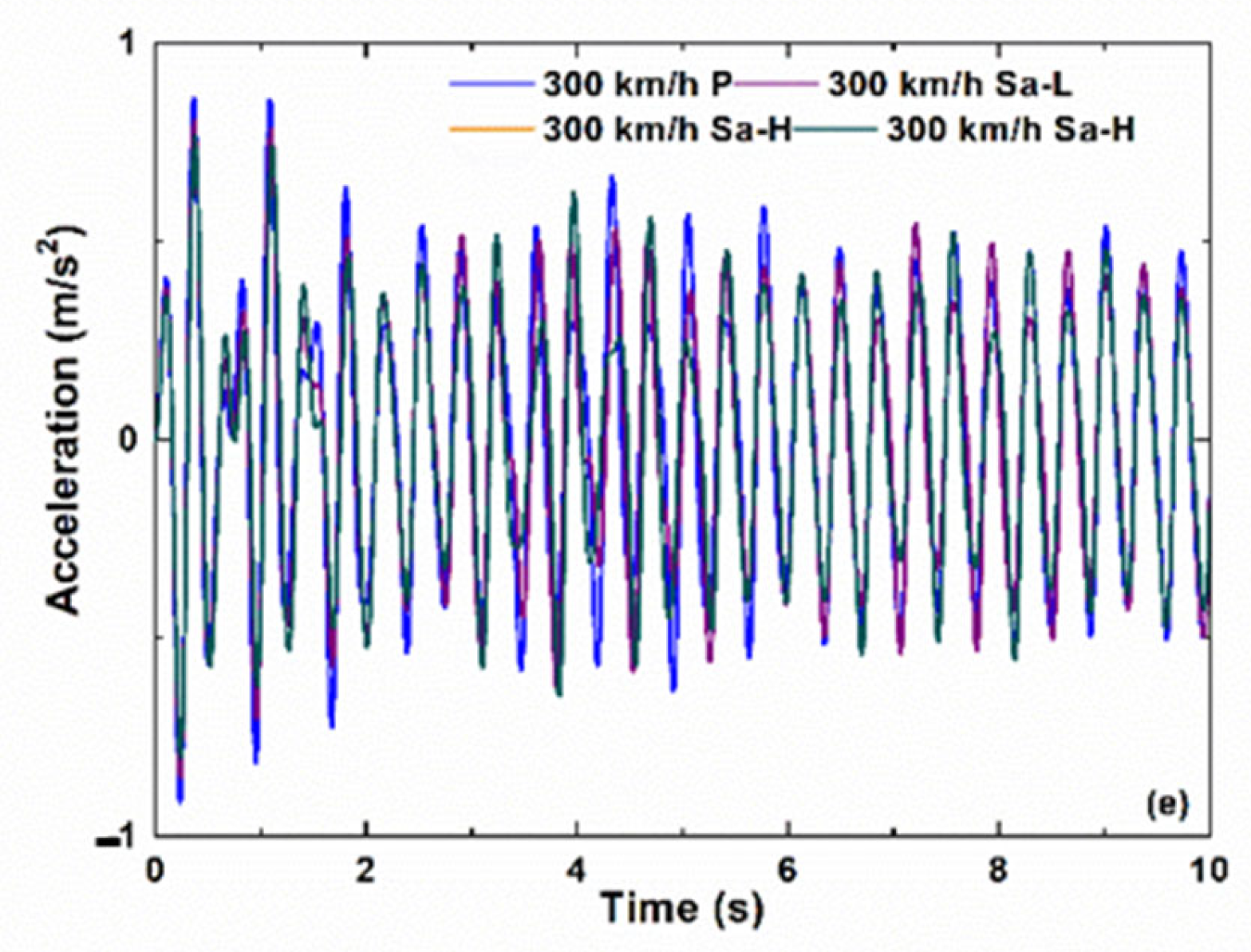
5.2.1. Acceleration Response Analysis

The acceleration response of the rail vehicle is a crucial indicator of how the suspension system performs in mitigating vibrations and external disturbances. To assess the system’s behavior, the acceleration was measured at different locations, particularly near the vehicle body’s mass center, under varying speeds, namely 60 km/h, 120 km/h, 180 km/h, 240 km/h, and 300 km/h.
Figure 16a–e illustrates the acceleration response near the CG of the carbody for the considered speeds. Each graph describes the acceleration behavior over time as the rail vehicle operates at different speeds. From the analysis, it has been observed (see Table 4) that the passive suspension system (PSS) exhibited relatively higher accelerations compared to the semi-active suspension systems (SaSS) across all speeds. At 60 km/h, the PSS, Sa-L, Sa-H, and Sa-C RMS accelerations were 0.29 m/s2, 0.28 m/s2, 0.27 m/s2, and 0.26 m/s2, respectively. As the speed increased to 300 km/h, the corresponding RMS accelerations were 0.60 m/s2, 0.56 m/s2, 0.55 m/s2, and 0.47 m/s2, respectively.
Moreover, the percentage reduction in RMS acceleration (PRI) was computed to quantify the effectiveness of the SaSS in reducing the rms acceleration. The results showed that the SaSS significantly improved compared to the PSS. For example, at 300 km/h, Sa-L, Sa-H, and Sa-C demonstrated a PRI of 6.67%, 8.93%, and 23.64%, respectively, signifying a considerable reduction in rms accelerations. The semi-active strategies, particularly Sa-C, showcased better performance in attenuating accelerations, making them more suitable for maintaining passenger comfort and safety.

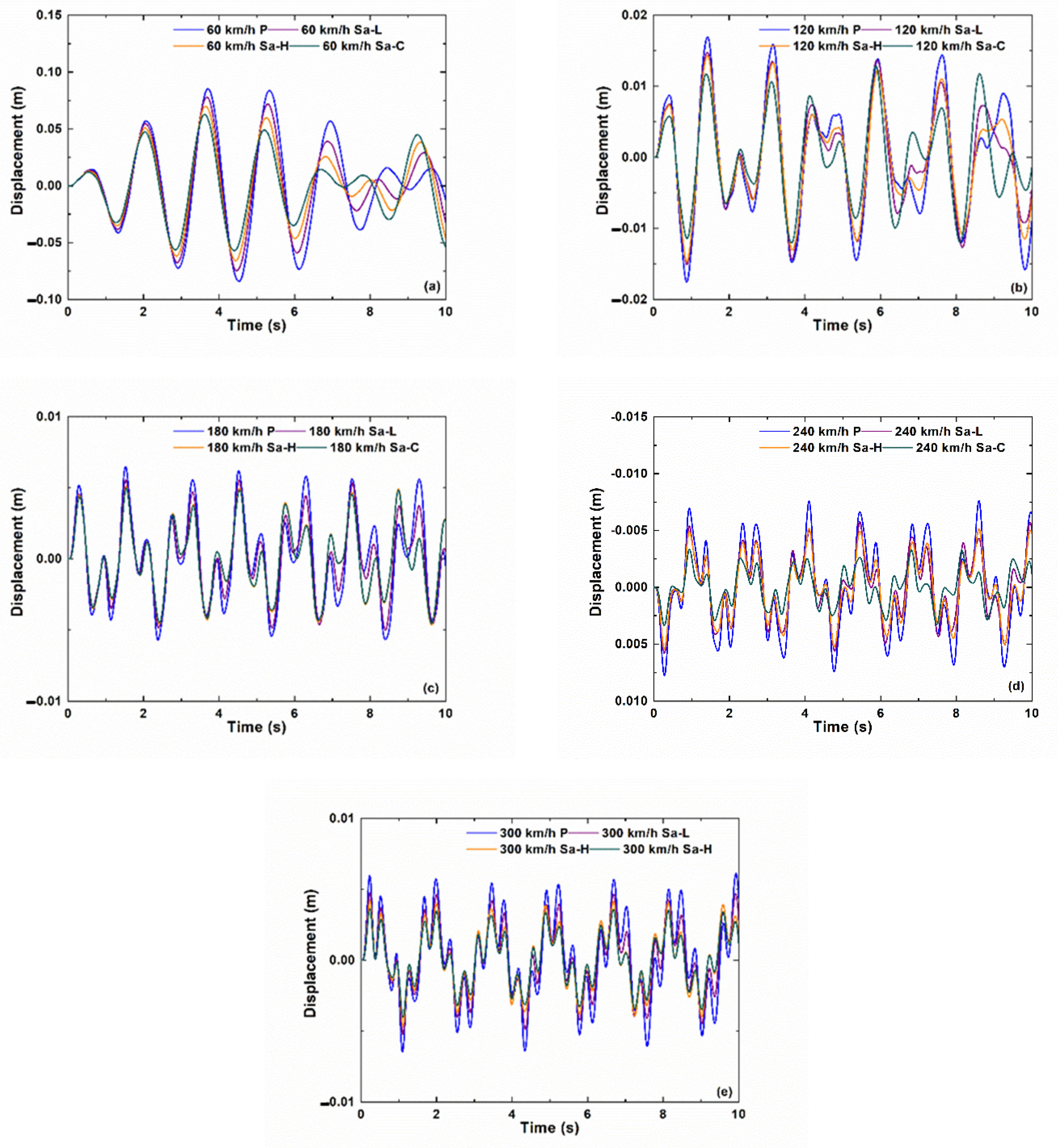
5.2.2. Displacement Response Analysis

The displacement response is another vital metric that directly influences the rail vehicle’s ride quality. Figure 17a–e presents the displacement response at the vehicle body’s center of mass for the considered speeds. Similar to the acceleration analysis, the displacement response was significantly influenced by the type of suspension system employed.
Table 5 shows the rms displacements for PSS, Sa-L, Sa-H, and Sa-C at 60 km/h were 2.89 mm, 2.84 mm, 2.80 mm, and 2.74 mm, respectively. As the speed increased to 300 km/h, the corresponding rms displacements were 3.90 mm, 3.44 mm, 3.15 mm, and 2.89 mm, respectively.
The SaSS also leads to a reduction in the RMS displacement PRI (Table 5). Specifically, it decreased 1.31–11.79% for Sa-L, 3.17–21.80% for Sa-H, and 5.36–32.06% for Sa-C, compared to PSS. This signifies that the SaSS can effectively mitigate the displacement response to external disturbances, enhancing ride comfort and reducing jarring sensations. Consequently, the findings demonstrate that the Sa-controlled suspension system significantly outperforms the PSS and the Sa-H and Sa-L suspension techniques.

5.3. Comparison of Ride Indices

Ride indices are essential statistical measures used to assess the performance of suspension systems in rail vehicles concerning ride quality and passenger comfort. This section extensively compares ride indices between the passive suspension system (PSS) and the semi-active suspension systems (SaSS).

5.3.1. Comparison of Ride Quality Index (RQI)

The Ride Quality Index (RQI) is a critical parameter that evaluates the smoothness and comfort of the rail vehicle’s ride. This paper considers the Sperling ride index method [29], in which a lower RQI indicates a smoother and more comfortable passenger ride experience. Table 6 presents the comparison of RQI for the different suspension strategies for different speeds. The results indicate that the semi-active suspension systems consistently provide better ride quality than the passive suspension system across all tested speeds. For instance, at 60 km/h, the RQIs for PSS, Sa-L, Sa-H, and Sa-C were 1.48, 1.38, 1.32, and 1.29, respectively. As the speed increased to 300 km/h, the corresponding RQIs were 3.26, 2.93, 2.74, and 2.41, respectively. The Sa-L, Sa-H, and Sa-C systems improve ride quality by around 5.75–10.53%, 6.71–18.72%, and 9.20–31.02%, respectively, compared to passive suspension. This suggests that SaSS can effectively reduce the impact of rail irregularities and vibrations, resulting in a smoother and more comfortable ride for passengers.
Table 6 shows that the Sa-C suspension system exhibited the lowest RQI, indicating that it delivers the smoothest ride quality among all suspension strategies. It is a significant advantage as passengers will likely experience a more pleasant and comfortable journey with Sa-C.

5.3.2. Comparison of Ride Comfort Index

The Ride Comfort Index is a quantitative measure used to assess the comfort level experienced by passengers during their journey in a rail vehicle. The PRI is an essential metric that measures the percentage reduction in vibration transmitted to the passenger’s body. A higher PRI implies a better reduction in discomfort caused by rail vibrations during the ride. Table 7 compares the PRI for the ride quality of the different suspension strategies. Similar to the RQI analysis, the semi-active suspension systems demonstrated superior performance in reducing vibration and improving passenger comfort compared to the passive suspension system. For instance, at 60 km/h, the ride comfort for PSS, Sa-L, Sa-H, and Sa-C was 2.44, 2.39, 2.31, and 2.21, respectively. As the speed increased to 300 km/h, the corresponding values were 3.41, 2.97, 2.8 and 2.58, respectively.
Table 7 also shows that the PRI for Sa-L, Sa-H, and Sa-C over PSS are 2.05–14.70%, 5.44–19.62%, and 9.96–31.50%, respectively. It is evident from the results that the SaSS, particularly Sa-H and Sa-C, consistently achieved higher PRI, indicating a better reduction in discomfort caused by rail vibrations. Passengers would probably feel less jarring sensations and greater comfort throughout their travel due to semi-active suspension systems.

6. Discussion

A novel and innovative approach for controlling the suspension of rail vehicles is represented by the SaSS, which is based on ANFIS. Integrating ANFIS technology with semi-active suspension systems results in a more versatile and adaptable solution than conventional passive suspension systems. ANFIS is a sophisticated hybrid computational model that combines the learning skills of neural networks with the reasoning powers of fuzzy logic. These two types of capabilities complement each other very well. Applications that need real-time control may make effective use of it because of its ability to adjust to shifting operation parameters quickly. The Bouc–Wen model is a magnetorheological (MR) damper used by the SaSS based on the ANFIS. This MR damper has settings that are always the same, guaranteeing that it will always behave the same regardless of the operating circumstances. The capacity of this option to react successfully to varied frequencies, excitation amplitudes, and current-level settings is the primary benefit that makes it advantageous. This enables it to be adapted to a variety of circumstances.

6.1. Performance Comparison with Other Methods

To evaluate the efficacy of the proposed ANFIS-based SaSS, a comparative analysis was performed against different suspension methods. The results demonstrated that the ANFIS-based SaSS outperformed the other systems across all tested conditions. Notably, the system exhibited notable improvements in reducing the root-mean-square (RMS) of acceleration and displacement compared to passive suspension systems and traditional semi-active strategies (Sa-H and Sa-L). The superior attenuation of acceleration and displacement responses indicates the ANFIS-based SaSS’s ability to effectively reduce the impact of rail irregularities and vibrations, resulting in a smoother and more comfortable ride for passengers. This enhanced performance makes the ANFIS-based SaSS a favorable choice for rail vehicle designers, manufacturers, and operators seeking to optimize ride quality and passenger comfort.

6.2. Adaptive Control and Dynamic Response

One of the main advantages of the ANFIS-based SaSS lies in its adaptive control capabilities. ANFIS can alter its control signals dynamically depending on real-time sensor input and vehicle operating circumstances. Because of its versatility, the system can react effectively to changing track conditions and various external disturbances, resulting in excellent suspension performance. The ANFIS-based SaSS’s dynamic reaction guarantees that passengers suffer minimum discomfort, even at fluctuating speeds and track conditions. The system’s capacity to react rapidly and correctly to exterior disturbances improves passenger safety and ride comfort.

6.3. Implications for Rail Vehicle Suspension Design

The research findings underscore the substantial implications of implementing the ANFIS-based SaSS in the design of rail vehicle suspension systems. The ANFIS-based SaSS offers a highly adaptive and responsive solution that effectively optimizes the performance and stability of the suspension system. It results in enhanced passenger comfort, reduced vibrations, and improved safety during rail travel. The ANFIS-based SaSS provides rail vehicle designers and manufacturers with an advanced solution to effectively tackle the issues related to ride quality and passenger comfort. The tool’s capacity to adjust to diverse operating conditions and promptly react to external disturbances renders it valuable in designing efficient and dependable suspension systems. Hence, the utilization of ANFIS-based SaSS substantially contributes to advancing rail vehicle suspension technology. Using ANFIS and an MR damper in a semi-active suspension system showcases notable advancements in enhancing ride quality, passenger comfort, and the overall rail travel experience. The system’s adaptive control capabilities and dynamic response render it a favorable choice for improving the performance and safety of rail vehicles.

7. Conclusions

In this paper, a comprehensive investigation into the effectiveness of an Adaptive Neuro-Fuzzy Inference System-based semi-active controlled suspension for high-speed rail vehicles was investigated. The investigation aims to address the critical challenges posed by different vibrations, i.e., lateral, vertical, yaw, roll motion, and track irregularities in passenger rail travel, ultimately enhancing comfort, safety, and ride stability. The findings of this paper highlight several significant contributions and critical observations. Firstly, the comparison of various suspension systems, including the Passive Suspension System (PSS) and different semi-active strategies (Sa-L, Sa-H, Sa-C), demonstrates that the SaSS consistently outperforms the PSS in terms of mitigating acceleration and displacement responses to external disturbances. The SaSS significantly reduces RMS acceleration and displacement and improves ride quality and comfort. Moreover, the evaluation of ride indices further reinforces the superiority of the SaSS in terms of ride quality and passenger comfort. The Sa-C systems achieve notable improvements, ranging from 9.20% to 31.02% in the ride quality index (Sperling ride index) and from 9.96% to 31.50% in the passenger comfort index. These findings demonstrate that the ANFIS-based semi-active controlled suspension effectively minimizes vibrations transmitted to passengers, resulting in smoother and more comfortable rides. The ANFIS-based controller’s adaptability and ability to dynamically respond to changes in track conditions make it a promising choice for effectively mitigating nonlinear vibrations and improving passenger comfort. Implementing the proposed semi-active controlled suspension system, integrated with the secondary vertical suspension, offers a more flexible and adaptive approach, which is particularly advantageous for modern high-speed trains with lighter bodies and an increased demand for comfort and safety.

Author Contributions

S.K.S. and R.C.S. prepared the inspection system for the experiment and performed the experiments presented in this research. J.L. conceived the original idea. J.L. designed the methodology, provided guidance, and helped improve the manuscript’s quality. S.K.S. wrote the original draft preparation in consultation with J.L. and Y.C., who reviewed and edited the final manuscript. All authors have read and agreed to the published version of the manuscript.

Funding

This work was supported by a National Research Foundation of Korea (NRF) grant funded by the Korean government (MSIT) (No. 2019R1A5A8083201) and Korea Institute of Energy Technology Evaluation and Planning (KETEP) grant funded by the Korean government (MOTIE) (20214000000480, Development of R&D engineers for combined cycle power plant technologies).

Data Availability Statement

Not applicable.

Conflicts of Interest

The authors declare no conflict of interest.

References

  1. Liu, C.; Chen, L.; Yang, X.; Zhang, X.; Yang, Y. General Theory of Skyhook Control and its Application to Semi-Active Suspension Control Strategy Design. IEEE Access 2019, 7, 101552–101560. [Google Scholar] [CrossRef]
  2. Jafari, B.; Mashadi, B. Valve control of a hydraulically interconnected suspension system to improve vehicle handling qualities. Veh. Syst. Dyn. 2023, 61, 1011–1027. [Google Scholar] [CrossRef]
  3. Fu, B.; Bruni, S. An examination of alternative schemes for active and semi-active control of vertical car-body vibration to improve ride comfort. Proc. Inst. Mech. Eng. Part F J. Rail Rapid Transit 2022, 236, 386–405. [Google Scholar] [CrossRef]
  4. Zhao, Y.; Liu, Y.; Yang, S.; Liao, Y.; Chen, Z. Analysis on new semi-active control strategies to reduce lateral vibrations of high-speed trains by simulation and hardware-in-the-loop testing. Proc. Inst. Mech. Eng. Part F J. Rail Rapid Transit 2022, 236, 960–972. [Google Scholar] [CrossRef]
  5. Fu, B.; Liu, B.; Di Gialleonardo, E.; Bruni, S. Semi-active control of primary suspensions to improve ride quality in a high-speed railway vehicle. Veh. Syst. Dyn. 2022, 1–25. [Google Scholar] [CrossRef]
  6. Chen, X.; Shen, L.; Hu, X.; Li, G.; Yao, Y. Suspension parameter optimal design to enhance stability and wheel wear in high-speed trains. Veh. Syst. Dyn. 2023, 1–23. [Google Scholar] [CrossRef]
  7. La Paglia, I.; Rapino, L.; Ripamonti, F.; Corradi, R. Modelling and experimental characterization of secondary suspension elements for rail vehicle ride comfort simulation. Proc. Inst. Mech. Eng. Part F J. Rail Rapid Transit 2023, 095440972311788. [Google Scholar] [CrossRef]
  8. Sun, X.; Wang, P.; Xu, J.; Xu, F.; Gao, Y. Simulation of the inherent structural irregularities of high-speed railway turnouts based on a virtual track inspection method. Proc. Inst. Mech. Eng. Part F J. Rail Rapid Transit 2023, 237, 114–123. [Google Scholar] [CrossRef]
  9. Yang, S.; Zhao, Y.; Liu, Y.; Liao, Y.; Wang, P. A new semi-active control strategy on lateral suspension systems of high-speed trains and its application in HIL test rig. Veh. Syst. Dyn. 2023, 61, 1317–1344. [Google Scholar] [CrossRef]
  10. Boada, M.J.L.; Calvo, J.A.; Boada, B.L.; Díaz, V. Modeling of a magnetorheological damper by recursive lazy learning. Int. J. Non. Linear. Mech. 2011, 46, 479–485. [Google Scholar] [CrossRef]
  11. Arias-Montiel, M.; Florean-Aquino, K.H.; Francisco-Agustin, E.; Pinon-Lopez, D.M.; Santos-Ortiz, R.J.; Santiago-Marcial, B.A. Experimental Characterization of a Magnetorheological Damper by a Polynomial Model. In Proceedings of the 2015 International Conference on Mechatronics, Electronics and Automotive Engineering (ICMEAE), Cuernavaca, Mexico, 24–27 November 2015; pp. 128–133. [Google Scholar]
  12. Dimock, G.A.; Yoo, J.-H.; Wereley, N.M. Quasi-Steady Bingham Biplastic Analysis of Electrorheological and Magnetorheological Dampers. J. Intell. Mater. Syst. Struct. 2002, 13, 549–559. [Google Scholar] [CrossRef]
  13. Sharma, S.K.; Sharma, R.C. Simulation of Quarter-Car Model with Magnetorheological Dampers for Ride Quality Improvement. Int. J. Veh. Struct. Syst. 2018, 10, 169–173. [Google Scholar] [CrossRef]
  14. Fang, Y. Optimal Control of Semiactive Two-Stage Vibration Isolation Systems for Marine Engines. Shock Vib. 2021, 2021, 5334670. [Google Scholar] [CrossRef]
  15. Maharani, E.T.; Ubaidillah, U.; Imaduddin, F.; Wibowo, W.; Utami, D.; Mazlan, S.A. A mathematical modelling and experimental study of annular-radial type magnetorheological damper. Int. J. Appl. Electromagn. Mech. 2021, 66, 543–560. [Google Scholar] [CrossRef]
  16. Han, Y.; Dong, L.; Hao, C. Experimental analysis and mathematical modelling for novel magnetorheological damper design. Int. J. Appl. Electromagn. Mech. 2019, 59, 367–376. [Google Scholar] [CrossRef]
  17. Kumar, A. Oscillation Trails on LHB Coach (AC Chair Car) in Palwal-Mathura Section of Central Railway upto a Maximum Test Speed of 180 KMPH on Rajdhani Track Maintained to Strandards Laid Down; Research Designs and Standards Organisation: Lucknow, India, 2000.
  18. Tupe, A.R. Handbook On Maintenance of Air Brake System in LHB Coaches (FTIL Type); Indian Railways, Centre for Advanced Maintenance Technology: Maharajpur, India, 2013.
  19. Vishnu, S.; Garg, S.; Singh, S.; Saha, S. Differential parametrization of rail vehicle properties and its impact on hunting. Proc. Inst. Mech. Eng. Part F J. Rail Rapid Transit 2023, 28, 09544097231184586. [Google Scholar] [CrossRef]
  20. Zhai, Z.; Zhu, S.; Yuan, X.; He, Z.; Cai, C. Nonlinear effects of a new mesh-type rail pad on the coupled vehicle-slab track dynamics system under extremely cold environment. Proc. Inst. Mech. Eng. Part F J. Rail Rapid Transit 2023, 237, 285–296. [Google Scholar] [CrossRef]
  21. Dominguez, A.; Sedaghati, R.; Stiharu, I. A new dynamic hysteresis model for magnetorheological dampers. Smart Mater. Struct. 2006, 15, 1179–1189. [Google Scholar] [CrossRef]
  22. Dyke, S.J.; Spencer, B.F.; Quast, P.; Kaspari, D.C.; Sain, M.K. Implementation of an Active Mass Driver Using Acceleration Feedback Control. Comput. Civ. Infrastruct. Eng. 1996, 11, 305–323. [Google Scholar] [CrossRef]
  23. Dyke, S.J.; Spencer, B.F.; Sain, M.K.; Carlson, J.D. Modeling and control of magnetorheological dampers for seismic response reduction. Smart Mater. Struct. 1996, 5, 565–575. [Google Scholar] [CrossRef]
  24. Al-Hmouz, A.; Shen, J.; Al-Hmouz, R.; Yan, J. Modeling and Simulation of an Adaptive Neuro-Fuzzy Inference System (ANFIS) for Mobile Learning. IEEE Trans. Learn. Technol. 2012, 5, 226–237. [Google Scholar] [CrossRef]
  25. Soni, T.; Das, A.S.; Dutt, J.K. Active vibration control of ship mounted flexible rotor-shaft-bearing system during seakeeping. J. Sound Vib. 2020, 467, 115046. [Google Scholar] [CrossRef]
  26. Nguyen, S.D.; Choi, S.-B.; Nguyen, Q.H. A new fuzzy-disturbance observer-enhanced sliding controller for vibration control of a train-car suspension with magneto-rheological dampers. Mech. Syst. Signal Process. 2018, 105, 447–466. [Google Scholar] [CrossRef]
  27. César, M.B.; Barros, R.C. ANFIS optimized semi-active fuzzy logic controller for magnetorheological dampers. Open Eng. 2016, 6, 518–523. [Google Scholar] [CrossRef]
  28. Sharma, S.K.; Sharma, R.C.; Lee, J.; Jang, H.-L. Numerical and Experimental Analysis of DVA on the Flexible-Rigid Rail Vehicle Carbody Resonant Vibration. Sensors 2022, 22, 1922. [Google Scholar] [CrossRef] [PubMed]
  29. Wang, Y.; Li, H.X.; Meng, H.D.; Wang, Y. Dynamic characteristics of underframe semi-active inerter-based suspended device for high-speed train based on LQR control. Bull. Pol. Acad. Sci. Tech. Sci. 2022, 70, 4. [Google Scholar] [CrossRef]
Figure 1. Schematic diagram represents a rail vehicle model equipped with a passive suspension system.
Sustainability 15 12529 g001
Figure 2. Spring Force—relative displacement characteristic for (a) primary vertical, (b) secondary vertical spring.
Sustainability 15 12529 g002
Figure 3. Damping Force—relative velocity damper characteristic for (a) primary vertical, (b) secondary vertical, (c) secondary lateral, and (d) secondary yaw damper.
Sustainability 15 12529 g003
Figure 4. MR damper according to a modified Bouc–Wen model.
Sustainability 15 12529 g004
Figure 5. The visual depicts the algorithm’s representation for MR damper force.
Sustainability 15 12529 g005
Figure 6. Illustrates the equivalent ANFIS reasoning mechanism for the Sugeno model, with different layers and node functions.
Sustainability 15 12529 g006
Figure 7. Velocity of the piston across the MR damper.
Sustainability 15 12529 g007
Figure 8. Comparison between the predicted current and target current.
Sustainability 15 12529 g008
Figure 9. Comparison between the predicted damping force and target damping force.
Sustainability 15 12529 g009
Figure 10. Two degrees of freedom rail vehicle system.
Sustainability 15 12529 g010
Figure 11. Circular wave of track irregularity.
Sustainability 15 12529 g011
Figure 12. Response of different controllers against considered circular track input.
Sustainability 15 12529 g012
Figure 13. Prototype coach for dynamic performance of rail vehicles.
Sustainability 15 12529 g013
Figure 14. Numerical—experimental comparison for (a) empty and (b) loaded.
Sustainability 15 12529 g014
Figure 15. Hysteresis force versus (a) velocity, (b) displacement, (c) time.
Sustainability 15 12529 g015
Figure 16. Acceleration response near the vehicle body’s mass center (a) 60 km/h, (b) 120 km/h, (c) 180 km/h, (d) 240 km/h, and (e) 300 km/h.
Sustainability 15 12529 g016aSustainability 15 12529 g016b
Figure 17. Displacement response at the vehicle body’s center of mass (a) 60 km/h, (b)120 km/h, (c) 180 km/h, (d) 240 km/h, and (e) 300 km/h.
Sustainability 15 12529 g017
Table 1. Parametric constants for the nonlinear suspension system.
ParameterValueParameterValue
a 1 −70,032.9 b 1 −40,703.7
a 3 1,182,302.18 b 3 4,898,875.651
a s z d 2.621 b s z d −0.00202
a s z d 26.929 b s z d 0.016387
a 2 8.60 b 2 27.31
a p z d 4.739 b p z d 7.63 × 10⁻⁵
a s y d 4.791 b s y d −0.00357
Table 2. Normalized errors in time, displacement, and velocity domains.
DisplacementVoltage (V)Time Span (s) E t E x E x ˙
GWN (0–2 Hz)GWN (0–2 Hz)100.08690.05730.1136
Table 3. Comparison of different controllers in terms of rise time, settling time, and overshoot.
Control SystemRise Time (ms)Settling Time (s)OvershootMax. Control Force (N)
Passive101.329.420472.2463-
PI261.693.5362868.9851075.08
PID181.242.481652.830541492.26
Fuzzy51.571.806236.26511786.42
ANFIS11.981.5920347.9067751394.34
Table 4. RMS acceleration and PRI for various suspension strategies.
SpeedRMS Acceleration (m/s2)PRI
km/hPassiveSa-LSa-HSa-CSa-LSa-HSa-C
600.290.280.270.263.457.1411.11
1200.350.320.320.318.579.3712.50
1800.470.430.410.388.5113.9521.95
2400.560.530.510.495.369.4313.73
3000.600.560.550.476.678.9323.64
Table 5. rms displacement and PRI for various suspension strategies.
SpeedRMS Displacement (mm)PRI
km/hPassiveSa-LSa-HSa-CSa-LSa-HSa-C
602.892.842.802.741.733.175.36
1203.053.012.922.781.314.329.25
1803.223.012.782.686.5214.6219.42
2403.353.122.982.716.8711.8621.48
3003.903.443.152.8911.7921.8032.06
Table 6. Comparison of Ride Quality Index (RQI) and Percentage Reduction Index (PRI) for different suspension strategies.
SpeedRide QualityPRI (Ride Quality)
km/hPassiveSa-LSa-HSa-CSa-LSa-HSa-C
601.481.381.321.296.7611.5914.39
1201.741.641.631.595.756.719.20
1801.961.841.791.686.129.2415.64
2402.091.871.741.5610.5318.7230.46
3003.262.932.742.4110.1217.7531.02
Table 7. Comparison of Ride Comfort Index and Percentage Reduction Index for different suspension strategies.
SpeedRide ComfortPRI (Ride Comfort)
km/hPassiveSa-LSa-HSa-CSa-LSa-HSa-C
602.442.392.312.212.055.449.96
1202.602.422.221.997.1315.9827.67
1802.612.362.272.219.8614.4617.79
2403.182.712.652.3414.7019.4031.50
3003.412.972.822.5812.8019.6229.42
Disclaimer/Publisher’s Note: The statements, opinions and data contained in all publications are solely those of the individual author(s) and contributor(s) and not of MDPI and/or the editor(s). MDPI and/or the editor(s) disclaim responsibility for any injury to people or property resulting from any ideas, methods, instructions or products referred to in the content.

