
Optimal Prediction of Wind Energy Resources Based on WOA—A Case Study in Jordan

 ,
,  ,
,  , and
, and 
Abstract
:1. Introduction
- In this paper, the mathematical model of wind analysis based on the Gamma distribution, which was infrequently utilized in the literature, has been derived;
- Using real examples, this paper provides technical comparisons between several types of wind distribution models: Weibull, Gamma, and Rayleigh distribution functions;
- The wind energy has been estimated for the designated wind sites using Weibull, Gamma, and Rayleigh distribution models.
2. Wind Data
2.1. Wind Speed Analysis
2.2. Wind Direction Analysis
3. Methodology
3.1. Wind Energy Fundamentals
3.2. Wind Distribution Models
3.2.1. Weibull Model
3.2.2. Rayleigh Model
3.2.3. Gamma Model
3.3. Wind Distribution Models Parameters Estimation
Whale Optimization Algorithm
- Establish the necessary parameters (N, Population size, Itermax) and then, initialize the population Xi (i = 1, 2..., N), as well as the coefficients a, A, C, l, and p;
- Assess the fitness of each search agent, and then choose X* as the ideal candidate;
- Update the following coefficients , , , and ;
- Determine the value. (I) If p < 0.5, then determine the value. (i) If , update the position by (7). (ii) Otherwise, if , select a random search agent Xrand and then, update the position by (14). (II) Otherwise, if p > 0.5, then update the position by (11);
- Verify that all whales (search agents) are taken into account. If not, move on to the next search agent; if yes, determine which search agents go over the search space and make the appropriate adjustments;
- Calculate the fitness for all search agents;
- Save the best solution X*.;
- Verify that the stopping criteria are met. If not, move on to step three; if yes, provide the optimal solution X* and its corresponding fitness score.
3.4. Performance Indicators
3.4.1. Root Mean Square Error
3.4.2. Coefficient of Determination
3.4.3. Mean Absolute Error
3.5. Wind Energy Estimation
3.6. Objective Function and Constraint
4. Results and Discussion
5. Conclusions
Author Contributions
Funding
Institutional Review Board Statement
Informed Consent Statement
Data Availability Statement
Acknowledgments
Conflicts of Interest
References
- Hoekman, S.K.; Broch, A.; Robbins, C.; Ceniceros, E.; Natarajan, M. Review of biodiesel composition, properties, and specifications. Renew. Sustain. Energy Rev. 2012, 16, 143–169. [Google Scholar] [CrossRef]
- REN21. Renewables 2020 Global Status Report; REN21 Secretariat: Paris, France, 2020; ISBN 978-3-948393-00-7. Available online: http://www.ren21.net/gsr-2020/ (accessed on 15 January 2021).
- Sathyajith, M. Wind Energy: Fundamentals, Resource Analysis and Economics, HAR/CDR ed.; Springer Medizin: Heidelberg, Germany, 2006. [Google Scholar]
- Boudia, S.M.; Benmansour, A.; Hellal, M.A.T. Wind resource assessment in Algeria. Sustain. Cities Soc. 2016, 22, 171–183. [Google Scholar] [CrossRef]
- Bidaoui, H.; El Abbassi, I.; El Bouardi, A.; Darcherif, A. Wind Speed Data Analysis Using Weibull and Rayleigh Distribution Functions, Case Study: Five Cities Northern Morocco. Procedia Manuf. 2019, 32, 786–793. [Google Scholar] [CrossRef]
- Salvação, N.; Soares, C.G. Wind resource assessment offshore the Atlantic Iberian coast with the WRF model. Energy 2017, 145, 276–287. [Google Scholar] [CrossRef]
- Bilir, L.; Imir, M.; Devrim, Y.; Albostan, A. Seasonal and yearly wind speed distribution and wind power density analysis based on Weibull distribution function. Int. J. Hydrogen Energy 2015, 40, 15301–15310. [Google Scholar] [CrossRef]
- Paraschiv, L.-S.; Paraschiv, S.; Ion, I.V. Investigation of wind power density distribution using Rayleigh probability density function. Energy Procedia 2019, 157, 1546–1552. [Google Scholar] [CrossRef]
- Shoaib, M.; Siddiqui, I.; Rehman, S.; Khan, S.; Alhems, L.M. Assessment of wind energy potential using wind energy conversion system. J. Clean. Prod. 2019, 216, 346–360. [Google Scholar] [CrossRef]
- Azad, K.; Rasul, M.; Halder, P.; Sutariya, J. Assessment of Wind Energy Prospect by Weibull Distribution for Prospective Wind Sites in Australia. Energy Procedia 2019, 160, 348–355. [Google Scholar] [CrossRef]
- Wang, J.; Huang, X.; Li, Q.; Ma, X. Comparison of seven methods for determining the optimal statistical distribution parameters: A case study of wind energy assessment in the large-scale wind farms of China. Energy 2018, 164, 432–448. [Google Scholar] [CrossRef]
- Gugliani, G.; Sarkar, A.; Ley, C.; Mandal, S. New methods to assess wind resources in terms of wind speed, load, power and direction. Renew. Energy 2018, 129, 168–182. [Google Scholar] [CrossRef]
- Wang, J.; Hu, J.; Ma, K. Wind speed probability distribution estimation and wind energy assessment. Renew. Sustain. Energy Rev. 2016, 60, 881–899. [Google Scholar] [CrossRef]
- Li, Y.; Huang, X.; Tee, K.F.; Li, Q.; Wu, X.-P. Comparative study of onshore and offshore wind characteristics and wind energy potentials: A case study for southeast coastal region of China. Sustain. Energy Technol. Assessments 2020, 39, 100711. [Google Scholar] [CrossRef]
- Saeed, M.A.; Ahmed, Z.; Yang, J.; Zhang, W. An optimal approach of wind power assessment using Chebyshev metric for determining the Weibull distribution parameters. Sustain. Energy Technol. Assessments 2019, 37, 100612. [Google Scholar] [CrossRef]
- Wahbah, M.; Feng, S.F.; El-Fouly, T.H.; Zahawi, B. Wind speed probability density estimation using root-transformed local linear regression. Energy Convers. Manag. 2019, 199, 111889. [Google Scholar] [CrossRef]
- Boro, D.; Thierry, K.; Kieno, F.P.; Bathiebo, J. Assessing the Best Fit Probability Distribution Model for Wind Speed Data for Different Sites of Burkina Faso. Curr. J. Appl. Sci. Technol. 2020, 71–83. [Google Scholar] [CrossRef]
- Jiang, H.; Wang, J.; Wu, J.; Geng, W. Comparison of numerical methods and metaheuristic optimization algorithms for estimating parameters for wind energy potential assessment in low wind regions. Renew. Sustain. Energy Rev. 2017, 69, 1199–1217. [Google Scholar] [CrossRef]
- Alrashidi, M.; Rahman, S.; Pipattanasomporn, M. Metaheuristic optimization algorithms to estimate statistical distribution parameters for characterizing wind speeds. Renew. Energy 2019, 149, 664–681. [Google Scholar] [CrossRef]
- Pishgar-Komleh, S.; Keyhani, A.; Sefeedpari, P. Wind speed and power density analysis based on Weibull and Rayleigh distributions (a case study: Firouzkooh county of Iran). Renew. Sustain. Energy Rev. 2015, 42, 313–322. [Google Scholar] [CrossRef]
- Serban, A.; Paraschiv, L.S.; Paraschiv, S. Assessment of wind energy potential based on Weibull and Rayleigh distribution models. Energy Rep. 2020, 6, 250–267. [Google Scholar] [CrossRef]
- Hu, Q.; Wang, Y.; Xie, Z.; Zhu, P.; Yu, D. On estimating uncertainty of wind energy with mixture of distributions. Energy 2016, 112, 935–962. [Google Scholar] [CrossRef]
- Dong, Y.; Wang, J.; Jiang, H.; Shi, X. Intelligent optimized wind resource assessment and wind turbines selection in Huitengxile of Inner Mongolia, China. Appl. Energy 2013, 109, 239–253. [Google Scholar] [CrossRef]
- Wu, J.; Wang, J.; Chi, D. Wind energy potential assessment for the site of Inner Mongolia in China. Renew. Sustain. Energy Rev. 2013, 21, 215–228. [Google Scholar] [CrossRef]
- Akgül, F.G.; Şenoğlu, B.; Arslan, T. An alternative distribution to Weibull for modeling the wind speed data: Inverse Weibull distribution. Energy Convers. Manag. 2016, 114, 234–240. [Google Scholar] [CrossRef]
- Aries, N.; Boudia, S.M.; Ounis, H. Deep assessment of wind speed distribution models: A case study of four sites in Algeria. Energy Convers. Manag. 2018, 155, 78–90. [Google Scholar] [CrossRef]
- Jung, C.; Schindler, D. Wind speed distribution selection—A review of recent development and progress. Renew. Sustain. Energy Rev. 2019, 114. [Google Scholar] [CrossRef]
- Chang, T.P. Estimation of wind energy potential using different probability density functions. Appl. Energy 2011, 88, 1848–1856. [Google Scholar] [CrossRef]
- Qin, Z.; Li, W.; Xiong, X. Estimating wind speed probability distribution using kernel density method. Electr. Power Syst. Res. 2011, 81, 2139–2146. [Google Scholar] [CrossRef]
- Xu, X.; Yan, Z.; Xu, S. Estimating wind speed probability distribution by diffusion-based kernel density method. Electr. Power Syst. Res. 2015, 121, 28–37. [Google Scholar] [CrossRef]
- Ammari, H.D.; Al-Rwashdeh, S.S.; Al-Najideen, M.I. Evaluation of wind energy potential and electricity generation at five locations in Jordan. Sustain. Cities Soc. 2015, 15, 135–143. [Google Scholar] [CrossRef]
- Habali, S.; Hamdan, M.; Jubran, B.; Zaid, A.I. Wind speed and wind energy potential of Jordan. Sol. Energy 1987, 38, 59–70. [Google Scholar] [CrossRef]
- Anani, A.; Zuamot, S.; Abu-Allan, F.; Jibril, Z. Evaluation of wind energy as a power generation source in a selected site in Jordan. Sol. Wind. Technol. 1988, 5, 67–74. [Google Scholar] [CrossRef]
- Amr, M.; Petersen, H.; Habali, S. Assessment of wind farm economics in relation to site wind resources applied to sites in Jordan. Sol. Energy 1990, 45, 167–175. [Google Scholar] [CrossRef]
- Habali, S.; Amr, M.; Saleh, I.; Ta’Ani, R. Wind as an alternative source of energy in Jordan. Energy Convers. Manag. 2001, 42, 339–357. [Google Scholar] [CrossRef]
- Abderrazzaq, M. Energy production assessment of small wind farms. Renew. Energy 2004, 29, 2261–2272. [Google Scholar] [CrossRef]
- Alghoul, M.A.; Sulaiman, M.Y.; Azmi, B.Z.; Wahab, M.A. Wind energy potential of Jordan. Int. Energy J. 2007, 8, 71–78. [Google Scholar]
- Bataineh, K.M.; Dalalah, D. Assessment of wind energy potential for selected areas in Jordan. Renew. Energy 2013, 59, 75–81. [Google Scholar] [CrossRef]
- Alsaad, M. Wind energy potential in selected areas in Jordan. Energy Convers. Manag. 2013, 65, 704–708. [Google Scholar] [CrossRef]
- Dalabeeh, A.S.K. Techno-economic analysis of wind power generation for selected locations in Jordan. Renew. Energy 2017, 101, 1369–1378. [Google Scholar] [CrossRef]
- Al-Ghriybah, M.; Fadhli, Z.M.; Hissein, D.D.; Mohd, S. Wind energy assessment for the capital city of Jordan, Amman. J. Appl. Eng. Sci. 2019, 17, 311–320. [Google Scholar] [CrossRef] [Green Version]
- Marashli, A.; Alburdaini, M.; Al-Rawashdeh, H.; Shalby, M. Statistical Analysis of Wind Speed Distribution Based on Five Weibull Methods for Wind Power Evaluation in Maan, Jordan. J. Energy Technol. Policy 2021, 11, 55–70. [Google Scholar] [CrossRef]
- Alsaqoor, S.; Marashli, A.; At-Tawarah, R.; Borowski, G.; Alahmer, A.; Aljabarin, N.; Beithou, N. Evaluation of Wind Energy Potential in View of the Wind Speed Parameters—A Case Study for the Southern Jordan. Adv. Sci. Technol. Res. J. 2022, 16, 275–285. [Google Scholar] [CrossRef]
- Al-Mhairat, B.; Al-Quraan, A. Assessment of Wind Energy Resources in Jordan Using Different Optimization Techniques. Processes 2022, 10, 105. [Google Scholar] [CrossRef]
- Al-Quraan, A.; Al-Mhairat, B. Intelligent Optimized Wind Turbine Cost Analysis for Different Wind Sites in Jordan. Sustainability 2022, 14, 3075. [Google Scholar] [CrossRef]
- Al-Quraan, A.; Al-Masri, H.; Al-Mahmodi, M.; Radaideh, A. Power curve modelling of wind turbines-A comparison study. IET Renew. Power Gener. 2021, 16, 362–374. [Google Scholar] [CrossRef]
- Al-Quraan, A.; Al-Masri, H.; Radaideh, A. New Method for Assessing the Energy Potential of Wind Sites-A Case Study in Jordan. Univers. J. Electr. Electron. Eng. 2020, 7, 209–218. [Google Scholar] [CrossRef]
- Al-Quraan, A.; Al-Mahmodi, M.; Radaideh, A.; Al-Masri, H.M.K. Comparative study between measured and estimated wind energy yield. Turk. J. Electr. Eng. Comput. Sci. 2020, 28, 2926–2939. [Google Scholar] [CrossRef]
- Elsner, P. Continental-scale assessment of the African offshore wind energy potential: Spatial analysis of an under-appreciated renewable energy resource. Renew. Sustain. Energy Rev. 2019, 104, 394–407. [Google Scholar] [CrossRef] [Green Version]
- Han, Q.; Ma, S.; Wang, T.; Chu, F. Kernel density estimation model for wind speed probability distribution with applicability to wind energy assessment in China. Renew. Sustain. Energy Rev. 2019, 115, 109387. [Google Scholar] [CrossRef]
- Kaplan, Y.A. Overview of wind energy in the world and assessment of current wind energy policies in Turkey. Renew. Sustain. Energy Rev. 2015, 43, 562–568. [Google Scholar] [CrossRef]
- Kazimierczuk, A.H. Wind energy in Kenya: A status and policy framework review. Renew. Sustain. Energy Rev. 2019, 107, 434–445. [Google Scholar] [CrossRef]
- Al-Quraan, A.; Al-Qaisi, M. Modelling, Design and Control of a Standalone Hybrid PV-Wind Micro-Grid System. Energies 2021, 14, 4849. [Google Scholar] [CrossRef]
- Radaideh, A.; Bodoor, M.; Al-Quraan, A. Active and Reactive Power Control for Wind Turbines Based DFIG Using LQR Controller with Optimal Gain-Scheduling. J. Electr. Comput. Eng. 2021, 2021, 1–19. [Google Scholar] [CrossRef]
- Ko, D.H.; Jeong, S.T.; Kim, Y.C. Assessment of wind energy for small-scale wind power in Chuuk State, Micronesia. Renew. Sustain. Energy Rev. 2015, 52, 613–622. [Google Scholar] [CrossRef]
- Ladenburg, J.; Hevia-Koch, P.; Petrović, S.; Knapp, L. The offshore-onshore conundrum: Preferences for wind energy considering spatial data in Denmark. Renew. Sustain. Energy Rev. 2020, 121, 109711. [Google Scholar] [CrossRef]
- Peters, J.L.; Remmers, T.; Wheeler, A.J.; Murphy, J.; Cummins, V. A systematic review and meta-analysis of GIS use to reveal trends in offshore wind energy research and offer insights on best practices. Renew. Sustain. Energy Rev. 2020, 128, 109916. [Google Scholar] [CrossRef]
- Everitt, B.; Skrondal, A. The Cambridge Dictionary of Statistics; Cambridge University Press: Cambridge, UK, 2002. [Google Scholar]
- Forbes, C.; Evans, M.; Hastings, N.; Peacock, B. Statistical Distributions, 4th ed.; Wiley: Hoboken, NJ, USA, 2010. [Google Scholar]
- Mirjalili, S.; Lewis, A. The Whale Optimization Algorithm. Adv. Eng. Softw. 2016, 95, 51–67. [Google Scholar] [CrossRef]
- Rosales-Asensio, E.; Borge-Diez, D.; Blanes-Peiró, J.-J.; Pérez-Hoyos, A.; Comenar-Santos, A. Review of wind energy technology and associated market and economic conditions in Spain. Renew. Sustain. Energy Rev. 2018, 101, 415–427. [Google Scholar] [CrossRef]
- Al-Quraan, A.; Alrawashdeh, H. Correlated Capacity Factor Strategy for Yield Maximization of Wind Turbine Energy. In Proceedings of the IEEE 5th International Conference on Renewable Energy Generation and Applications (ICREGA), Al-Ain, United Arab Emirates, 26–28 February 2018. [Google Scholar]
- Al-Quraan, A.; Stathopoulos, T.; Pillay, P. Comparison of wind tunnel and on site measurements for urban wind energy estimation of potential yield. J. Wind. Eng. Ind. Aerodyn. 2016, 158, 1–10. [Google Scholar] [CrossRef] [Green Version]
- Brano, V.L.; Orioli, A.; Ciulla, G.; Culotta, S. Quality of wind speed fitting distributions for the urban area of Palermo, Italy. Renew. Energy 2011, 36, 1026–1039. [Google Scholar] [CrossRef]
- Al-Quraan, A.; Al-Mahmodi, M.; Al-Asemi, T.; Bafleh, A.; Bdour, M.; Muhsen, H.; Malkawi, A. A New Configuration of Roof Photovoltaic System for Limited Area Applications—A Case Study in KSA. Buildings 2022, 12, 92. [Google Scholar] [CrossRef]
- Wimhurst, J.J.; Greene, J.S. Oklahoma’s future wind energy resources and their relationship with the Central Plains low-level jet. Renew. Sustain. Energy Rev. 2019, 115, 109374. [Google Scholar] [CrossRef]
- Al-Addous, M.; Saidan, M.; Bdour, M.; Dalala, Z.; Albatayneh, A.; Class, C.B. Key aspects and feasibility assessment of a proposed wind farm in Jordan. Int. J. Low-Carbon Technol. 2019, 15, 97–105. [Google Scholar] [CrossRef] [Green Version]


| Study | Candidate Site(s) | Study Period | Data Resolution | Distribution Model(s) | Estimation Method(s) | Performance Indicator(s) | Study Objective(s) | |
|---|---|---|---|---|---|---|---|---|
| Study in Ref. [37] | Amman | Aqaba | 9 years | Daily | Weibull | Graphical method | Kolmogorov–Smirnov | For wind regime:
|
| Irbid | Der Alla | |||||||
| Ras Monief | ||||||||
| Study in Ref. [38] | Hofa | Tafila | 2–4 years 9 years (Fujaij) | Monthly | Rayleigh | Direct computing of parameter (c) based on mean speed | N/A | For proposed 4 models of WTs:
|
| Ibrahimya | Fujaij | |||||||
| Zabda | Aqaba | |||||||
| Ras Monief | ||||||||
| Study in Ref. [39] | Alhassan Industrial City | 20 years | Monthly | N/A | N/A | N/A | For proposed wind farm:
| |
| Fujaij | ||||||||
| Safawi | ||||||||
| Ras Monief | ||||||||
| Study in Ref. [31] | Azraq | Q. A. Airport * | 5 years | 6 h | Weibull | Standard deviation method | N/A | For proposed 5 models of WTs:
|
| Safawi | K. H. Airport ** | |||||||
| Ras Monief | ||||||||
| Study in Ref. [40] | Amman | 9 years | Daily | Weibull | Graphical method | N/A | For proposed 4 models of WTs:
| |
| Irbid | ||||||||
| Aqaba | ||||||||
| Der Alla | ||||||||
| Ras Monief | ||||||||
| Study in Ref. [41] | Amman | 7 years | N/A | Weibull | Trend of k vs. | N/A | For wind regime:
| |
| Study in Ref. [42] | Ma’an | 1 year | Daily | Weibull Rayleigh | Graphical method Empirical method Moment method Energy pattern factor method | RMSE X2 test R2 MPE MAPE | For wind regime:
| |
| Study in Ref. [43] | Ma’an | 1 year | 10 min | Weibull Rayleigh | Empirical method Moment method Energy pattern factor method | N/A | For wind regime:
| |
| Aqaba | ||||||||
| Batn Elghol | ||||||||
| Proposed Study | Q. A. Airport * | Mafraq | 1 year | 1 h, 3 h and 6 h | Gamma Weibull Rayleigh | Artificial intelligent method (WOA) Moment method Maximum likelihood method | RMSE R2 MAE | For wind regime:
|
| K. H. Airport ** | Ma’an | |||||||
| A. C. Airport *** | Safawi | |||||||
| Irbid | Irwaished | |||||||
| Ghor El Safai | ||||||||
| Latitude | Longitude | Elevation | Number of Data | Sampling Rate | Period | |
|---|---|---|---|---|---|---|
| Queen Alia Airport | 31.43° N | 35.59° E | 722 m | 7173 | 1 h | 01/2019–12/2019 |
| Amman Civil Airport | 31.59° N | 35.59° E | 767 m | 6910 | 1 h | 09/2018–08/2019 |
| King Hussein Airport | 29.33° N | 35.00° E | 51 m | 6711 | 1 h | 01/2018–12/2018 |
| Irbid | 32.33° N | 35.51° E | 618 m | 899 | 6 h | 03/2018–02/2019 |
| Mafraq | 32.22° N | 36.15° E | 686 m | 1909 | 3 h | 09/2018–08/2019 |
| Ma’an | 30.10° N | 35.47° E | 1069 m | 1014 | 6 h | 03/2018–02/2019 |
| Safawi | 32.09° N | 37.12° E | 647 m | 1703 | 3 h | 01/2018–12/2018 |
| Irwaished | 32.30° N | 38.12° E | 686 m | 764 | 6 h | 09/2017–08/2018 |
| Ghor El-Safi | 31.02° N | 35.28° E | −350 m | 790 | 6 h | 01/2018–12/2018 |
| No. of Class | Speed Class (m/s) | Wind Speed Observations (%) | ||||||||
|---|---|---|---|---|---|---|---|---|---|---|
| Queen Alia Airport | Amman Civil Airport | King Hussein Airport | Irbid | Mafraq | Ma’an | Safawi | Irwaished | Ghor El-Safi | ||
| 1 | 0.04 | 0.04 | 0.00 | 0.11 | 0.00 | 0.00 | 0.00 | 0.13 | 0.13 | |
| 2 | 3.14 | 14.20 | 0.58 | 43.60 | 5.08 | 1.68 | 0.29 | 6.15 | 34.68 | |
| 3 | 23.67 | 23.00 | 12.71 | 40.04 | 31.53 | 18.84 | 8.69 | 26.05 | 41.14 | |
| 4 | 16.94 | 18.47 | 16.36 | 11.12 | 20.53 | 32.64 | 24.78 | 20.29 | 13.42 | |
| 5 | 12.46 | 13.98 | 16.41 | 3.67 | 15.61 | 18.93 | 19.55 | 14.27 | 6.20 | |
| 6 | 16.23 | 12.59 | 16.38 | 1.22 | 12.05 | 10.06 | 15.97 | 13.09 | 3.04 | |
| 7 | 10.25 | 7.71 | 16.87 | 0.11 | 7.86 | 3.55 | 9.51 | 8.64 | 1.01 | |
| 8 | 8.43 | 4.60 | 13.80 | 0.00 | 4.66 | 4.44 | 5.58 | 3.53 | 0.25 | |
| 9 | 2.89 | 2.14 | 3.89 | 0.11 | 1.10 | 5.92 | 6.46 | 3.53 | 0.00 | |
| 10 | 2.27 | 1.19 | 2.21 | 0.00 | 0.79 | 1.18 | 4.17 | 1.44 | 0.00 | |
| 11 | 1.74 | 0.90 | 0.52 | 0.00 | 0.26 | 0.79 | 3.41 | 0.26 | 0.00 | |
| 12 | 0.70 | 0.64 | 0.18 | 0.00 | 0.10 | 0.79 | 0.70 | 0.65 | 0.00 | |
| 13 | 0.50 | 0.41 | 0.01 | 0.00 | 0.26 | 0.39 | 0.53 | 0.92 | 0.00 | |
| 14 | 0.25 | 0.07 | 0.00 | 0.00 | 0.05 | 0.49 | 0.12 | 0.65 | 0.00 | |
| 15 | 0.49 | 0.07 | 0.09 | 0.00 | 0.10 | 0.30 | 0.23 | 0.39 | 0.13 | |
| Site | Occurrence Rate (%) | Overall (%) | |||||||
|---|---|---|---|---|---|---|---|---|---|
| N | NW | W | SW | S | SE | E | NE | ||
| Queen Alia Airport | 1.87 | 26.20 | 27.42 | 17.50 | 2.17 | 8.02 | 7.17 | 9.66 | 100 |
| Amman Civil Airport | 4.15 | 29.32 | 21.49 | 26.66 | 0.87 | 4.67 | 5.70 | 7.13 | 100 |
| King Hussein Airport | 68.55 | 16.69 | 1.00 | 4.04 | 3.46 | 2.09 | 0.36 | 3.82 | 100 |
| Irbid | 3.67 | 14.24 | 33.93 | 25.14 | 2.00 | 15.68 | 4.12 | 1.22 | 100 |
| Mafraq | 5.61 | 51.23 | 7.44 | 16.66 | 2.83 | 14.35 | 1.20 | 0.68 | 100 |
| Ma’an | 7.50 | 41.32 | 15.38 | 15.98 | 8.19 | 6.31 | 2.27 | 3.06 | 100 |
| Safawi | 14.15 | 22.49 | 18.03 | 24.13 | 7.11 | 7.69 | 3.35 | 3.05 | 100 |
| Irwaished | 7.46 | 20.55 | 15.71 | 16.36 | 12.30 | 11.65 | 8.90 | 7.07 | 100 |
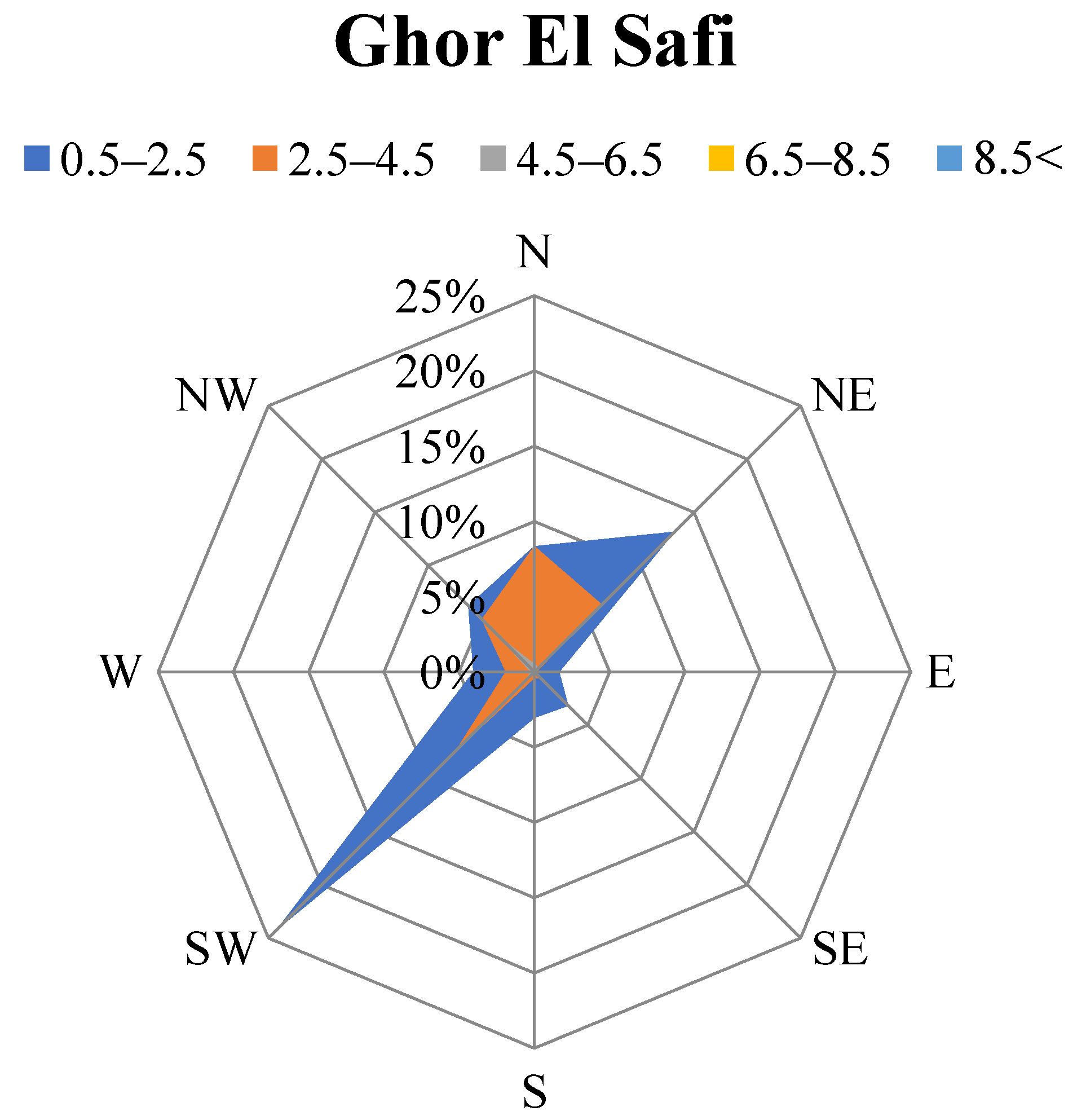
| Ghor El-Safi | 17.22 | 14.56 | 6.20 | 32.53 | 3.42 | 4.43 | 1.77 | 19.87 | 100 |
| Average | 14.46 | 26.29 | 16.29 | 19.89 | 4.70 | 8.32 | 3.87 | 6.17 | 100 |
| Site | Parameter and Indicator | Estimation Methods | ||||||||
|---|---|---|---|---|---|---|---|---|---|---|
| W-MM | W-MLM | W-WOA | R-MM | R-MLM | R-WOA | G-MM | G-MLM | G-WOA | ||
| Queen Alia Airport | K | 2.326 | 2.075 | 2.013 | 2.000 | 2.000 | 2.000 | 4.771 | 4.172 | 4.051 |
| C | 6.564 | 5.272 | 5.012 | 4.641 | 3.697 | 3.369 | 1.219 | 1.114 | 1.013 | |
| RMSE | 0.03919 | 0.02846 | 0.0254 | 0.03738 | 0.02904 | 0.02690 | 0.03620 | 0.02488 | 0.02223 | |
| R2 | 0.68313 | 0.83287 | 0.88272 | 0.71169 | 0.82599 | 0.87527 | 0.72965 | 0.87232 | 0.90230 | |
| MAE | 0.02157 | 0.01502 | 0.01312 | 0.02201 | 0.01546 | 0.01446 | 0.01768 | 0.01417 | 0.01140 | |
| Amman Civil Airport | K | 3.609 | 4.277 | 1.503 | 2.000 | 2.000 | 2.000 | 1.940 | 2.191 | 0.541 |
| C | 5.750 | 4.492 | 4.231 | 4.063 | 3.201 | 4.903 | 1.190 | 1.098 | 1.034 | |
| RMSE | 0.03796 | 0.01848 | 0.01548 | 0.03537 | 0.01809 | 0.01711 | 0.03454 | 0.01082 | 0.01013 | |
| R2 | 0.73523 | 0.93727 | 0.95721 | 0.77006 | 0.93985 | 0.94912 | 0.78082 | 0.97849 | 0.98836 | |
| MAE | 0.02514 | 0.00900 | 0.00700 | 0.02368 | 0.00944 | 0.00821 | 0.02161 | 0.00725 | 0.00425 | |
| King Hussein Airport | K | 3.011 | 2.806 | 2.515 | 2.000 | 2.000 | 2.000 | 7.636 | 6.339 | 5.323 |
| C | 6.397 | 5.640 | 3.550 | 4.559 | 3.800 | 2.98500 | 0.748 | 0.791 | 0.6820 | |
| RMSE | 0.02012 | 0.01760 | 0.01588 | 0.02886 | 0.03012 | 0.02746 | 0.02147 | 0.02257 | 0.01734 | |
| R2 | 0.91378 | 0.93402 | 0.94362 | 0.82265 | 0.80674 | 0.84612 | 0.90186 | 0.89149 | 0.92164 | |
| MAE | 0.01092 | 0.00993 | 0.00793 | 0.02192 | 0.01663 | 0.01561 | 0.01272 | 0.01201 | 0.01002 | |
| Irbid | K | 2.795 | 2.462 | 2.122 | 2.000 | 2.000 | 2.000 | 6.664 | 6.588 | 6.211 |
| C | 2.798 | 2.379 | 2.139 | 1.988 | 1.618 | 1.521 | 0.374 | 0.320 | 0.282 | |
| RMSE | 0.06894 | 0.04226 | 0.03226 | 0.08108 | 0.07409 | 0.05409 | 0.04504 | 0.02086 | 0.01883 | |
| R2 | 0.83109 | 0.93653 | 0.94631 | 0.76638 | 0.80491 | 0.84123 | 0.92790 | 0.98453 | 0.99123 | |
| MAE | 0.03991 | 0.02789 | 0.02289 | 0.06006 | 0.04231 | 0.02385 | 0.02457 | 0.01490 | 0.01291 | |
| Mafraq | K | 2.361 | 2.090 | 1.890 | 2.000 | 2.000 | 2.000 | 4.904 | 4.757 | 4.451 |
| C | 5.385 | 4.269 | 4.166 | 3.808 | 2.987 | 2.612 | 0.973 | 0.792 | 0.721 | |
| RMSE | 0.04008 | 0.03073 | 0.02661 | 0.03933 | 0.03214 | 0.03014 | 0.03464 | 0.02310 | 0.02011 | |
| R2 | 0.72736 | 0.83973 | 0.86952 | 0.73735 | 0.82462 | 0.84455 | 0.79629 | 0.90938 | 0.92912 | |
| MAE | 0.01718 | 0.01169 | 0.01069 | 0.01751 | 0.01246 | 0.01146 | 0.01311 | 0.01062 | 0.00805 | |
| Ma’an | K | 2.279 | 2.033 | 2.012 | 2.000 | 2.000 | 2.000 | 4.595 | 4.592 | 4.582 |
| C | 6.183 | 4.868 | 4.561 | 4.370 | 3.428 | 3.122 | 1.192 | 0.934 | 0.832 | |
| RMSE | 0.06074 | 0.04812 | 0.03322 | 0.05982 | 0.04869 | 0.03511 | 0.05256 | 0.03512 | 0.03222 | |
| R2 | 0.54047 | 0.71168 | 0.79451 | 0.55439 | 0.70478 | 0.78422 | 0.65602 | 0.84639 | 0.91539 | |
| MAE | 0.03774 | 0.02848 | 0.02122 | 0.03806 | 0.02873 | 0.02273 | 0.03076 | 0.01889 | 0.01711 | |
| Safawi | K | 2.566 | 2.312 | 2.212 | 2.000 | 2.000 | 2.000 | 5.704 | 5.276 | 5.076 |
| C | 6.917 | 5.783 | 5.645 | 4.900 | 3.974 | 3.734 | 1.077 | 0.967 | 0.912 | |
| RMSE | 0.04550 | 0.03341 | 0.03134 | 0.04481 | 0.03832 | 0.02823 | 0.03743 | 0.02301 | 0.02014 | |
| R2 | 0.63002 | 0.80052 | 0.82023 | 0.64109 | 0.73750 | 0.85712 | 0.74963 | 0.90537 | 0.91533 | |
| MAE | 0.02877 | 0.02152 | 0.01812 | 0.03046 | 0.02536 | 0.01501 | 0.02198 | 0.01515 | 0.01112 | |
| Irwaished | K | 2.150 | 1.908 | 1.815 | 2.000 | 2.000 | 2.000 | 4.135 | 3.797 | 3.297 |
| C | 6.216 | 4.764 | 4.264 | 4.393 | 3.412 | 3.112 | 1.332 | 1.107 | 1.007 | |
| RMSE | 0.04821 | 0.03268 | 0.03034 | 0.04692 | 0.03135 | 0.03134 | 0.04243 | 0.02286 | 0.01823 | |
| R2 | 0.62109 | 0.82588 | 0.83512 | 0.64098 | 0.83977 | 0.83912 | 0.70653 | 0.91482 | 0.93401 | |
| MAE | 0.02869 | 0.01941 | 0.01701 | 0.02854 | 0.01859 | 0.01801 | 0.02517 | 0.01388 | 0.01312 | |
| Ghor El-Safi | K | 1.729 | 1.676 | 1.476 | 2.000 | 2.000 | 2.000 | 2.779 | 4.757 | 4.351 |
| C | 5.087 | 2.683 | 2.483 | 3.617 | 2.065 | 2.012 | 1.631 | 0.503 | 0.493 | |
| RMSE | 0.06149 | 0.04152 | 0.03834 | 0.06466 | 0.03221 | 0.02821 | 0.05802 | 0.01457 | 0.01150 | |
| R2 | 0.48583 | 0.76558 | 0.73523 | 0.43145 | 0.85895 | 0.91895 | 0.54215 | 0.97114 | 0.98110 | |
| MAE | 0.02501 | 0.01203 | 0.01012 | 0.02592 | 0.01091 | 0.00991 | 0.02363 | 0.00481 | 0.00388 | |
| ET (kWh/m2) | |||||||||
|---|---|---|---|---|---|---|---|---|---|
| Method | Numerical | AI | Numerical | AI | Numerical | AI | |||
| MM | MLM | WOA | MM | MLM | WOA | MM | MLM | WOA | |
| Site | Queen Alia Airport | Amman Civil Airport | King Hussein Airport | ||||||
| Weibull | 1002.32 | 1006.72 | 1150.85 | 634.64 | 668.45 | 809.34 | 910.87 | 992.54 | 1066.74 |
| Rayleigh | 1005.82 | 1019.06 | 1319.76 | 653.56 | 661.49 | 792.66 | 1080.98 | 1106.81 | 1228.51 |
| Gamma | 930.56 | 988.21 | 1070.26 | 622.21 | 662.62 | 862.92 | 1002.21 | 1029.35 | 1140.65 |
| Site | Irbid | Ma’an | Mafraq | ||||||
| Weibull | 76.55 | 80.38 | 109.58 | 488.60 | 530.80 | 630.93 | 780.64 | 809.05 | 915.65 |
| Rayleigh | 81.21 | 85.47 | 113.77 | 502.45 | 537.65 | 577.55 | 802.88 | 812.81 | 890.41 |
| Gamma | 70.3 | 75.7 | 98.51 | 420.22 | 493.92 | 603.73 | 705.23 | 739.93 | 825.12 |
| Site | Safawi | Irwaished | Ghor El-Safi | ||||||
| Weibull | 1190.99 | 1209.17 | 1369.33 | 164.89 | 172.17 | 194.25 | 165.74 | 172.17 | 192.84 |
| Rayleigh | 1202.65 | 1265.83 | 1295.95 | 158.92 | 177.7 | 201.22 | 155.56 | 177.70 | 189.52 |
| Gamma | 1121.43 | 1170.33 | 1250.82 | 116.22 | 126.36 | 192.71 | 122.76 | 126.36 | 168.71 |
Disclaimer/Publisher’s Note: The statements, opinions and data contained in all publications are solely those of the individual author(s) and contributor(s) and not of MDPI and/or the editor(s). MDPI and/or the editor(s) disclaim responsibility for any injury to people or property resulting from any ideas, methods, instructions or products referred to in the content. |
© 2023 by the authors. Licensee MDPI, Basel, Switzerland. This article is an open access article distributed under the terms and conditions of the Creative Commons Attribution (CC BY) license (https://creativecommons.org/licenses/by/4.0/).
Share and Cite
Al-Quraan, A.; Al-Mhairat, B.; Malkawi, A.M.A.; Radaideh, A.; Al-Masri, H.M.K. Optimal Prediction of Wind Energy Resources Based on WOA—A Case Study in Jordan. Sustainability 2023, 15, 3927. https://0-doi-org.brum.beds.ac.uk/10.3390/su15053927
Al-Quraan A, Al-Mhairat B, Malkawi AMA, Radaideh A, Al-Masri HMK. Optimal Prediction of Wind Energy Resources Based on WOA—A Case Study in Jordan. Sustainability. 2023; 15(5):3927. https://0-doi-org.brum.beds.ac.uk/10.3390/su15053927
Chicago/Turabian StyleAl-Quraan, Ayman, Bashar Al-Mhairat, Ahmad M. A. Malkawi, Ashraf Radaideh, and Hussein M. K. Al-Masri. 2023. "Optimal Prediction of Wind Energy Resources Based on WOA—A Case Study in Jordan" Sustainability 15, no. 5: 3927. https://0-doi-org.brum.beds.ac.uk/10.3390/su15053927